A knowledge-based prognostics framework for railway track geometry degradation

Contents lists available atScienceDirect

Reliability Engineering and System Safety

journal homepage:www.elsevier.com/locate/ress

A knowledge-based prognostics framework for railway track geometry

degradation

Juan Chiachío

a,⁎

_{, Manuel Chiachío}

a,b

_{, Darren Prescott}

a

_{, John Andrews}

a

a_{Resilience Engineering Research Group, University of Nottingham, Nottingham NG7 2RD, UK}

b_{Department of Structural Mechanics and Hydraulics Engineering, University of Granada, Spain}

A R T I C L E I N F O

Keywords:

Railway track degradation Physics-based modelling Prognostics

Particle filtering

A B S T R A C T

This paper proposes a paradigm shift to the problem of infrastructure asset management modelling by focusing towards forecasting the future condition of the assets instead of using empirical modelling approaches based on historical data. The proposed prognostics methodology is general but, in this paper, it is applied to the particular problem of railway track geometry deterioration due to its important implications in the safety and the main-tenance costs of the overall infrastructure. As a key contribution, a knowledge-based prognostics approach is developed by fusing on-line data for track settlement with a physics-based model for track degradation within a filtering-based prognostics algorithm. The suitability of the proposed methodology is demonstrated and dis-cussed in a case study using published data taken from a laboratory simulation of railway track settlement under cyclic loads, carried out at the University of Nottingham (UK). The results show that the proposed methodology is able to provide accurate predictions of theremaining useful lifeof the system after a model training period of about 10% of the process lifespan.

1. Introduction

In most developed countries, the continuous ageing and the growing demand of use of critical infrastructures calls for advanced Prognostics and Health Management (PHM) concepts for optimal infrastructure asset management[1]. In particular for the railway infrastructure, the continuous deterioration of the track due to traffic loading represents the main ageing factor requiring periodic interventions to restore the track to an acceptable geometry[2,3]. These maintenance interventions not only represent a significant part of the railway operation expenses, but also imply temporary line closures and a reduction of the effective network capacity, so they need to be planned months in advance. It is in this context of anticipated decision making where the benefits of PHM can be fully exploited for maintenance cost optimization and downtime reduction.

As evident from the literature, railway track degradation and maintenance modelling to date has a strong empirical retrospective character, mainly grounded on data-based (stochastic or phenomen-ological) models with limited prospective capability. A systematic re-view of these models is proposed by Dahlberg[4]for track settlement modelling, and more recently by Soleimanmeigouni et al. [5] and Higgins and Liu[6]focusing also in track maintenance modelling. The prediction accuracy of those models strongly depends on the quality

and quantity of the available historic data, and thus they are prone to misjudgements especially under medium-to-long term future sce-narios. To overcome this limitation, some physics-based models have been proposed to predict the progressive mechanical degradation of the track under cyclic loadings from first geomechanical principles, like the cyclic densification model by Suiker and de Borst[7], and the elasto-plastic models by Indraratna et al. [8] and more recently by Sunet al. [9]. The referred physics-based models are transparent to human understanding and they can adapt to different material and loading conditions without much training, which is essential to confer the required early predictive capability. However, they are unable to account for the uncertainty in the predictions since they are based on deterministic input-output relationships. In this context, a number of authors have adopted statistical methods to quantify the modelling uncertainty in track geometry degradation, such as regression ana-lysis[10], stochastic processes[11–13], Markov models[14,15], and Bayesian analysis[16], to cite but a few. Notwithstanding, as stated before, the accuracy of these methods relies almost entirely on histor-ical data, which bounds their prospective capability and the reliability of their predictions.

In this paper, a paradigm shift for track geometry degradation modelling and maintenance is proposed. Instead of making main-tenance decisions based on either a retrospective data-based modelling

https://doi.org/10.1016/j.ress.2018.07.004

Received 1 December 2017; Received in revised form 24 June 2018; Accepted 4 July 2018

⁎_{Corresponding author.}

E-mail address:[email protected](J. Chiachío).

Available online 05 July 2018

0951-8320/ © 2018 The Authors. Published by Elsevier Ltd. This is an open access article under the CC BY license (http://creativecommons.org/licenses/BY/4.0/).

of the track, or, alternatively, using a purely deterministic physics-based approach, aknowledge-basedprognostics framework is proposed herein. This approach fuses information from physics-based models and available data about track degradation within a Bayesian learning paradigm to sequentially reduce the initial modelling uncertainty[17] as long as new data are collected, so as to obtain increasingly accurate forecasts of the future condition of the track. These forecasts enable the testing of various load and utilisation scenarios, and more importantly, allow us to answer the question of ”when will failure occur” with quantified uncertainty. The proposed methodology enables informed, anticipated, and risk-based decisions about optimal railway track asset management, and can be extended to other railway assets to enable decision-making at a system infrastructural level. To the authors’ best knowledge, the existing literature on track degradation prognostics is currently limited to Mishra et al.[18], focusing on railway switches based on a phenomenological model for track geometry degradation.

For the problem of physical modelling of the track deterioration, an elasto-plastic model for track settlement is developed based on first principles of the plasticity of soils[19]and Critical State Soil Mechanics (CSSM) [20]. This model provides the temporal evolution of the ele-mentary volumetric and deviatoric plastic strains of the track based on some geomechanical inputs. Apart from the traffic loads, the inputs required by the model reduce to thecritical state parameters[20], which can be obtained from routine triaxial tests, and two uncertain para-meters controlling the cyclic hardening of the granular layers of the track, which are sequentially updated using condition monitoring data. For the sake of Bayesian data assimilation, the proposed model is embedded within a hidden Markov model [21]where the deviatoric and volumetric plastic strains constitute thelatent states, and the ver-tical permanent axial strain is the observed state. Next, a sequential Bayesian updating framework is used to update both the latent states and the uncertain model parameters as long as new data become available. The resulting equations for sequential updating are analyti-cally intractable, hence a Sequential Monte Carlo approach based on particle filters[22]is adopted whereby the probability density functions (PDFs) are approximated by weighted samples or particles, which re-present random realisations of the updated track degradation states. Finally, by extrapolating those particles into the future, a prob-ability-based estimation of the time (load cycles) to reach a predefined functional limit for track degradation is subsequently obtained. This time defines what in the Prognostics and Health Management com-munity is commonly known as theremaining useful life(RUL)[1]of the system.

As a case study, the proposed methodology is tested against ex-perimental data taken from Aursudkijet al.[23]about permanent axial strain in a ballasted railway track, carried out at the Nottingham Railway Test Facility[24]. The results show that the proposed prog-nostics methodology is able to accurately anticipate the future states of deformation of the track after a training period of about 10% of the total length of the process, which corresponds to the time required by the model to assimilate the data. This prognostics performance is compared with the performance obtained for the same dataset using an empirical logarithmic model for track settlement. The assessment is carried out using a newly developed prognostics metric named as the relative prospective evidence, which measures the relative prediction ac-curacy of two different model classes in relation to the amount of in-formation that the models need to extract from the data to perform their predictions. The results show that the physics-based model proposed in this paper is the one with the larger and earlier anticipation capacity, needing less support from condition monitoring data to make accurate prognostics estimates.

The remainder of the paper is organised as follows.Section 2 pre-sents the physical fundamentals behind the proposed model for track deterioration. Section 3 overviews the mathematical basis and com-putational aspects of Bayesian state estimation and prognostics, which have been both specialised for their application to the railway track

degradation problem. InSection 4, the proposed framework is applied to railway track settlement data to serve as a case study. A discussion about the suitability of model-based prognostics for railway track maintenance planning is provided inSection 5. Finally,Section 6 pro-vides concluding remarks.

2. Physics-based model for track settlement

A constitutive model for ballast plastic deformation under cycling loading is developed here following the general theory of plasticity, CSSM, and Pender’s postulates about plastic deformation of over-consolidated soils[25]. The model predicts the evolution of the plastic vertical strain p

1 of a representative track section, which is the variable of interest here, whereby the settlement of the section can be straightforwardly derived. The reader is referred to[25]for a detailed overview of the foundations of the proposed model, but for the sake of clarity, the key formulation and definitions are reproduced here with a uniform notation.

2.1. Physical fundamentals

Following the theory of plasticity, a granular medium under a stress state represented by the stress tensorσij, will experience an increment in the plastic strains given by Hill’sflow rule[26], as

= dijp h gdf

ij (1)

wheredijpis the corresponding plastic strain increment tensor,dfis the differential of function f, which denotes the yield criterion (or yield surface),gis theplastic potential, andhis thehardening function. These elements are briefly explained inDefinitions 1to3, respectively. If the stress invariantspandq are adopted instead of the stress tensorσij, Eq. (1)can be rewritten as:

=

d h g

pdf

vp

(2a)

=

d h g

qdf

s p

(2b) with vpand sp being the corresponding plastic volumetric and distor-tional strain invariants. The reader is referred toAppendix Afor further insight about stress and strains invariants. Having vpand spas known, the vertical plastic strain of the track section can be straightforwardly computed as:

=1/3 + p

vp sp

1 (3)

as shown inEq. (A.4b)inAppendix A. It follows that functionsf, gandh need to be determined so as to define a closed-form expression for the constitutive model inEq. (2).

Definition 1 (Yield criterion[19]).The yield criterion defines the limit of the elastic behaviour and the onset of plastic deformation under any possible combination of stresses. Mathematically:f p q( , )=0.

Assuming Pender’s hypothesis that overconsolidated soils experi-ence plastic strain only when there is a change in the stress ratio ( =q p/ )[25], the yield criterion can be assumed to be given by:

= =

f q _ip 0 ₍₄₎

whereηidefines a particular constant stress ratio yield locusi(refer to Fig. 2 in [25]). By differentiating Eq. (4), df=dq _idp, and sub-stitutingdq= _idp+pd obtained from the definition ofη, the required

expression fordfinEq. (2)can be shown to be given by: =

df pd (5)

generic expression g p q( , )=0 and relates the incremental plastic strains with the stress state following the plastic flow rule inEq. (1).

An analytical expression forgcan be obtained by noting that the plastic strains are normal to the plastic potentialg p q( , )=0,thus im-plying that[19]:

= d d

dq dp

vp

s

p ₍₆₎

In this research, the ratiod vp/dspis assumed to be given by a modified version of Rowe’s stress-dilatancy model[27], as

= + d d

M

M M

9( *)

9 3 2 *

vp s

p ₍₇₎

whereMis the slope of thecritical state linein thep qspace[28], and

η* is a function of the stress ratio given by *= p p/ ,cs withpcsbeing

defined inEq. (13)below. The stress-dilatancy criterion inEq. (7) dif-fers from that proposed by Rowe[27]in that it provides positive values for plastic volumetric strain increments (i.e., contraction), as long asη*

does not exceed the critical state valueM. By substitutingEq. (7)into (6)and solving the resulting differential equation, an expression for the plastic potential function is obtained, as:

= + + + =

g p q( , ) 3 ln( / )M p C (2M 3)ln(2 * 3) (3 M)ln(3 *) 0

(8) whereCis an integration constant.

Definition 3 (Hardening function[19]).As a work hardening material, ballast experiences a dynamical change of its plastic response during yielding. This change is accomplished by modifying the yield surface as plastic flow occurs. The hardening function (h inEq. (2)) accounts for such effect.

An expression forhcan be obtained following the premise that no volume change takes place during undrained deformation[20]. Math-ematically:

= + =

d v d ve d vp 0 (9)

wheredevis the elastic volumetric strain increment given by[20]

= +

d dp

p(1 e) v

e

0 (10)

with κ being the swelling/recompression constant. By substituting Eqs. (2a)and(10)intoEq. (9),his obtained as:

= +

h e

dp p

g ppd

1 0

1

(11) InEq. (11), Pender’s assumption of parabolic undrained stress paths in thep qspace[25]is adopted to relate the stress derivativesdpand dη. This assumption is expressed as:

= M

p p

p p p p

1 /

1 /

cs

cs

0 0

2

0

0 (12)

whereη₀is the initial stress ratio (corresponding to the minimum load

within the cycle),p0is the initial value of the mean stress invariantp,

andpcsis the value ofpat the point on the critical state line corre-sponding to the current voids ratioe, obtained as[28,29]:

=

p_cs exp e

cs (13)

with Γ andλcsbeing material parameters. These parameters, together withMandκ(see nomenclatureTable A.3), are thecritical state para-meters of the model and can be evaluated from a series of drained triaxial compression tests [30]. Having obtained the differential dp usingEq. (12), and substituting it intoEq. (11), the hardening function

becomes after some algebraic manipulation1_:

= +

+

h p p p p

e M p p

M M

M d

2 (1 / )( / )( )

(1 )( ) (2 / 1)

9 3 2 *

9( *)

cs cs

0 0

0 02 0 (14)

It should be emphasised that the last equation is nominally valid for the first load cycle. For subsequent loading,hshould account for other complex phenomena observed in experiments under cyclic loading conditions, such as the Bauschinger effect, the effect of the stress ratio and loading history, etc.[19]. A semi-empirical approach is adopted here to account for such processes following Indraratna and Salim[8], which essentially consists of multiplying the hardening function in Eq. (14)by a semi-empirical factorϕgiven by

= +

+ M

p p q q

p p q q n

1 *

( ) ( )

e e

max min max min

2 2

2 2

1/2

(15) whereαandβare empirical fitting parameters,nis the accumulated number of cycles, ⟨ · ⟩ are the Macauley brackets, andpeis given by the expression[8]:

= +

+

p p

n p p

1 1

ln( 10) ( )

e min max min

(16) with pmin and pmax being the minimum and maximum mean stress

invariant within load cyclen, respectively. The corresponding devia-toric componentsq_min,q_max andqeare obtained usingEq. (A.4a), de-fined inAppendix A.

2.2. Constitutive equations of proposed model

Substituting the expressions forf, gandhobtained above intoEq. (2), and after some algebraic manipulation, the following expressions for the evolution of the plastic volumetric and deviatoric strains are obtained:

+ = =

d d

p p p p

e M p p

2 (1 / )( / )( )

(1 )( ) (2 / 1) 0, ( ) ( ) v

p

n

cs cs

n v p

n vp max n

0 0

0 02 0 0

1

(17a) +

= =

d d

M M

M

d d

9 3 2 *

9( *) 0, ( ) ( )

s p

vp

n

sp 0 n sp max n 1

(17b) where · |n denotes a variable evaluated at load cycle n, and

=q /p

max max max. Note that for thenth loading cycle, the initial condition for both deviatoric and volumetric plastic strains is given by the corre-sponding plastic strains at the previous cyclen 1. The initial conditions

( )

v p

0 0 and sp( )0 0 are assumed as known. Observe also that the

ex-pressions inEq. (17)are non-linear differential equations of the plastic strains, thus they need to be integrated numerically by replacing the de-rivatives by their finite difference approximation (e.g., using explicit Euler method). An algorithmic description of the numerical method proposed to integrate the constitutiveEqs. (17a)and(17b)is presented inAlgorithm 1.

3. Track-degradation prognostics

Prognostics is concerned with predicting the future state of health of engineering systems or components given the current degree of wear or damage, and, based on that, estimating the remaining time in which the system is expected to continue performing its intended function within desired specifications [1]. The predictions are carried out using no additional evidence but a sequence of measurements up to the time of prediction, and the available models for system behaviour. A physics-based filtering-physics-based prognostics framework is proposed herein as de-picted inFig. 1. The definitions inSection 3.1are used to provide the

Input:

σ

3

{Confining

pressure};

[M

,λ

c s

,

Γ

,κ

]

{critical

state

parameters};

α,

β

{fitting

parameters};

σ

1 , min

,σ

1 , ma x

{min,

max

v

ertical

stress};

n

{#

of

load

cycles};

N

S

{#

of

in-c

ycle

load

steps};

e v

|

0

{initial

elastic

v

olumetric

strains};

e

|

0

{initial

v

oids

ratio};

h

p

v

|

n

,

p

|

s

n

i

{plastic

strains

after

n

cycles};

e

|

n

{v

oids

ratio

after

n

cycles}

Output:

h

p

v

|

n+

1

,

p

|

s

n + 1

i

{plastic

strains

at

n

+

1};

e

|

n+

1

{v

oids

ratio

at

n

+

1}

Begin: 1:

Set

min

and

max

de

viatoric

stresses:

q

min

,

q

max

T

=

|

σ

1 , min

−

σ

3

|

,

|

σ

1 , ma x

−

σ

3

|

2:

Set

min

and

max

mean

stresses:

p

min

,

p

max

T

=

1

/

3

q

min

,

q

max

T

+

σ

3

[1

,

1

]

T 3:

Set

in-c

ycle

stress

increments

∆

p

,

∆

q

T

=

p

max

,

q

max

T

−

p

min

,

q

min

T

/

N

S 4:

Set

initial

stress

state

q

0

,

p

0

=

q

min

,

p

min

5:

Set

initial

v

oids

ratio:

e

i=

1

←

e

|

n 6:

for

i

=

1

to

N

S

do

7:

Obtain

(p

c s

)

i

=

p

c s

(e

i

)

from

Eq.

(13)

8:

Obtain

(p

0

)

i

=

p

0

(q

i

,

p

i

,

(p

c s

)

i

)

from

Eq.

(12)

9:

Compute

stress

state:

p

i

,

q

i

T

=

p

i − 1

,

q

i−

1

T

+

∆

p

,

∆

q

T 10:

Set

stress

ratio

increment:

∆

η

i

=

qi pi

−

qi−

1

pi−

1

11:

Obtain

(d

e v

/

d

p

)

i

from

Eq.

(10)

12:

Compute

v

olumetric

elastic

strain:

(

e v

)

i

=

(

e v

)

i − 1

+

(d

e v

/

d

p

)

i

∆

p

13:

Compute

h

(d

p

/

v

d

η

|

n

)

i

,

(d

p

/

s

d

η

|

n

)

i

i

from

Eqs.

(17a)

and

(17b)

14:

Compute

plastic

strains:

h

(

p

)

v

i

,

(

p

)

s

i

i

T

=

h

(

p

)

v

i − 1

,

(

p

)

s

i − 1

i

T

+

h

(d

p

/

v

d

η

)

i

,

(d

p

/

s

d

η

)

i

i

∆

η

i

[1

,

1

]

T 15:

Obtain

total

v

olumetric

strain:

(

v

)

i

=

(

p

)

v

i

+

(

e v

)

i 16:

Update

the

v

oids

ratio

e

i+

1

=

e

0

−

(1

+

e

0

)(

v

)

i 17:

end

for

18:

h

e

|

n

+

1

,

p

|

v

n

+

1

,

p

|

s

n

+

1

i

←

h

e

N

S

,

(

p

)

v NS

,

(

required mathematical background about prognostics in the context of the track degradation problem investigated here.

3.1. Fundamentals about model-based prognostics

Definition 4 (Hidden Markov model[21]).A hidden Markov model is a

time-series model comprised of a couple of discrete-time stochastic processes, namely {xn}n≥ 0 and {yn}n≥ 0. The former is an unobserved Markov

process described by the state vector xntaking values in a space denoted by , with known prior PDF π(x0) and transition density given by

x x

( n n 1),non necessarily Gaussian. The process{yn}n≥ 0 represents a

[image:5.595.100.501.54.265.2]

sequence of noisy observations taking values in ,which are assumed Fig. 1.Schematic overview of the proposed prognostics framework.

[image:5.595.74.521.303.613.2]

to be conditionally independent given the states xn.

A discrete-time state-space representation is typically adopted to describe the hidden Markov model, as follows[1]:

= +

xn fn(xn 1, ,un) n (18a)

= +

y_n g_n( , ,xn un) wn (18b)

where fn: nu× nx× n nx is the state transition equation, re-presented by a possibly nonlinear function of the state variablexnalong with a setu nu of input parameters to the system (loadings,

geo-mechanical inputs, etc.). The function g_n: nu× nx× n ny de-notes theobservation equationand provides the expected observation or measurementyngiven the hidden statexn. Both functionsfandgmay depend on a set of uncertain model parameters n _(e.g.,

fit-ting parameters). The terms n nx and wn ny in Eq. (18) are

stochastic variables that represent the modelling error and the mea-surement error, respectively. Supported by the Principle of Maximum Information Entropy[31],νnandwncan be conservatively modelled as zero-mean Gaussian distributions[1]. Thus, the state space model de-fined inEq. (18)can be probabilistically rewritten as2_:

=

x x f

( n n 1, ) ( ( 1, ), ) (19a)

=

y x g

(_n n, ) ( ( , ), ) (19b)

where n nx×x and ×

w n ny y are the covariance matrices of the

model error and the measurement error, respectively. Note inEq. (19) and in what follows that the conditioning on the model inputsunis dropped for simpler notation.

In this work, the (latent) state of the system at loading cyclen is assumed to be described by the plastic deviatoric and volumetric strains, i.e., xn=(spn, vpn) 2, where subscripts (s, v) denote the

deviatoric and volumetric components, respectively. The observations of the system are assumed to be given by the vertical plastic strain, yn= 1pn , which can be theoretically estimated from the component plastic strains usingEq. (3). Under these assumptions, the covariance matrices for the error terms are given by

=_{diag( , )} ×

s v

, , 2 2for the model error, and w= w for the measurement error, withσν,sandσν,vbeing respectively the standard deviations of the deviatoric and volumetric components of the model error, and σwthe standard deviation of the measurement error. With these settings, the deterministic physics-based model proposed in Section 2isstochastically embeddedwithin a hidden Markov model by defining the functionsfandginEqs. (19a)and(19b), as:

=

x f f

fn( n 1, ) ( (s psn 1, ), (v vpn 1, )) (20a)

= +

g 1

3 n sp

n v

p

n (20b)

where functionsfsandfvinEq. (20a)are given by

= +

f_s(spn 1, ) spn 1 spn( ) (21a)

= +

f_v(vpn 1, ) vpn 1 vpn( ) (21b)

In the last equation, spnand vpnare the increments in the plastic

deviatoric and volumetric strains within loading cycle n, respectively. These strain increments can be obtained as:

= =

d d s vp

n j

N s vp

n j j

,

1 ,

Eq.(17)

S

(22)

where subscripts (s, v) denote the deviatoric and volumetric compo-nents, respectively, andNS is the number of discretising steps of the loading ramp at cyclen(the unloading ramp is regarded as elastic). The reader is referred toAlgorithm 1for details about the numerical com-putation of the plastic deviatoric and volumetric strains for load cyclen.

Definition 5 (Sequential state estimation).The sequential estimation of the track degradation aims at obtaining an updated estimation of the actual condition of the track based on available measurements up to cycle n. The degradation is described by the state variable xnalong with the uncertain model parameters θ, leading to an augmented state variable

= +

zn ( , )xn nx n. Thus, given a sequence of track degradation measurements, denoted asy_1:n { , ,y₁ y_{n 1}, },y_n the goal is to obtain the most plausible sequence of track degradation statesz0:n { , ,z0 zn 1,zn} for those measurements, which is given by Bayes’ Theorem as[1]:

=

z y y z z y

y z z y dz

y z z z z y

( ) ( ) ( )

( ) ( )

( ) ( ) ( )

n n n n n n

n n n n n

n n n n n n

0: 1: 0: 1: 1

0: 1: 1 0:

Eq. (19b)

1 0: 1 1: 1

last update (23)

where =

z z x x

(n n 1) ( n n 1, n) ( n n )

Eq. (19a)

1

(24)

Observe fromEq. (24)that model parametersθnare virtually time-evolving although they are essentially not dependent on time, which is a key problem that typically arises when sequentially updating the state variable as an augmented state[32]. A common solution is to add a white-noise perturbation to the set of updated parameters at timen 1 before evolving to the next predicted state at time n, i.e., n= n 1+ n, where n (0, n). This induces a

Markovian-type artificial dynamics to the model parameters whereby the required PDF ( n n 1)is prescribed[32,33], as follows:

=

( n n 1) ( n 1, n) (25)

where is a covariance matrix specified here as =diag

(

2 , , 2 , , 2

)

,

n n,1 n j, n n, with 2n j, being the variance of the

random walk of thejth component of the parameter vectorθat time or cyclen. Note that such artificial evolution imposes a loss of information in θ over time (e.g., increasingly larger spread inπ(z0:n|y1:n)) since additional uncertainties are artificially added to the model para-meters. Several methods have been proposed in the literature to over-come this drawback, with the most popular being those that impose a shrinkage over nas long as new data are available[32]. An efficient

method of this class is adopted in this work[34], which consists in sequentially modifying the variances 2 , j=1, , ,n

n j, as follows:

= 1 P*RMAD( ) RMAD* RMAD( )

j n j j

n j

2 2 ,

,

n j, n 1,j

(26) where RMAD(θn, j) is the relative median absolute deviation of π(θn, j|y1:n),RMAD*j is the target RMAD forπ(θn, j|y1:n), andP*j [0, 1] is a scaling constant that controls the speed of convergence to RMAD*_j. BothRMAD*_j andP*_j need to be tuned by the modeller. A comprehensive discussion about the optimal choice forP*_j andRMAD*_j

is found in[34].

Definition 6 (Predicted system state).Given the most up-to-date assessment of the system at time or cycle n, π(zn|y1:n), a probability-based prediction of the future states of degradation of the system ℓ-steps forward in time can be obtained by Total Probability Theorem as[1,35]:

= +

= + +

+

z y z z z y dz

(n n) ( ) ( )

t n n

t t n n n n

1:

1

1 1: : 1

(27)

whereℓ> 1 is the number of prediction steps in absence of new data, and (z zt t 1)is the state transition equation defined inEq. (24), which, fort>n, encloses the future behaviour of the system.

To numerically solve this multi-dimensional integral, an approx-imation can be readily obtained byconditional sampling, using recur-sively the one-step transition equation defined in(24), i.e.: first sample

+

zn( )i1using the aforementioned one-step transition equation conditional

on the initial statezn, i.e.,zn( )i+1 (·zn); then sample the succeeding

state conditional on the previous sample, i.e.,zn( )+i2 (·zn( )+i1); finally, repeat the same process until the target timen+ is reached.

Definition 7 (End of Life (EOL)[1]).The EOL is defined as the earliest time or loading cycle t>n when the predicted event[zt ]takes place,

where zt∼π(zt|y1:n) and is the subset of states where the system behaviour becomes unacceptable.

In the context of the proposed track degradation problem, re-presents the set of values for the vertical plastic strain exceeding the threshold ,which delimits the boundary between thefailure region and the safe region = . Observe that since the predicted statesztare uncertain (recallEq. (27)), the EOL will be an uncertain variable distributed according to the PDFπ(EOLn|y1:n). This PDF can be theoretically obtained as the distribution of the predicted states con-tained in the boundary ,i.e., (EOLny1:n) (zt y1:n),given that[t=EOL ]n [zt ]. It follows that (zn+ y1:n)can be

written as a conditional PDF (zn+ y1:n, ),which can be evaluated

as:

= =

+

z y y k z y z

( n 1:n, ) (EOLn 1:n) ( t 1:n) ( )t

Eq.(27) (28)

wherekis a normalising constant and ( )zt is an indicator function

that assigns the unity if(zt ),and makes zero the rest.

Definition 8 (Remaining Useful Life (RUL)[1]).The RUL is the remaining time in which the system is foreseen to perform within the region of acceptable performance, where = , the non-empty subset of authorised states of the system. A prediction of the RUL from the time of prediction n can be straightforwardly obtained from EOLn as

= n

RULn EOLn .

Definition 9 (Prospective evidence for a model). Given a degradation process nobserved up to current time or load cycle n, and a particular model class which idealises such a process (e.g., the one proposed in

Section 2), the prospective evidence for model class is the probability of the subsequent degradation process, denoted as _n+, to be predicted by .The prospective evidence can be obtained by Total Probability Theorem as:

=

+ + d

( n n, ) ( n n, n, ) (n n, ) n ₍₂₉₎

where ( n n, ) is the marginal posterior of the model

para-meters at load cyclen, given byEq. (23), and ( _n+ _n, _n, )is the prospective likelihood function, which measures how likely _n+ is pre-dicted by model class parameterized byθn. The computation of this likelihood function along with the estimation of the multidimensional integral inEq. (29)are explained inAppendix B.

Note that for this definition, data for the future degradation process +are assumed to be known, which holds true for offline and pseudo-online prognostics analyses, but it could be a hard assumption in a purely online prognostics scenario. In that case, we assume that +can be available through experiments run in similar conditions or by the existence of repeated tests.

3.2. Algorithms for prognostics

The methodology for track degradation prognostics explained above involves the evaluation of multidimensional integrals (recallEqs. (23) and(27), respectively) which are analytically intractable, except for

some of especial linear cases using Gaussian uncertainties[22]. Ap-proximating methods like Sequential Monte Carlo[22]are required to overcome those integrals by numerical approximation. In prognostics, these approximating methods are typically integrated within algorithms which (1) sequentially estimate the joint PDF of states and model parameters as long as new data are collected, referred to as particle filteringalgorithms, and (2) extrapolate the updated state estimations into the future in absence of new observations until the EOL is reached. Depending upon implementation both algorithms may not be separable, however, for the sake of clarity, they will be presented here separately inSections 3.2.1and3.2.2, respectively.

3.2.1. Sequential state estimation algorithm

With particle filters, the PDF of the most up to date state of de-gradation of the trackπ(z0:n|y1:n) can be approximated through a set of Nweightedparticlesor samples{z0:( )in, n( )i}iN=1,as:

=

z y z z

( n n) ( )

i N

ni n in

0: 1:

1 ( )

0: 0:( )

(30) whereδis the Dirac delta and _iN n( )i =1. The value of the particle weights{ ni}i=

N ( )

1can be obtained bysequential importance sampling[22] each time a new data point arrives, as explained in the pseudocode given asAlgorithm 2. Note that a systematic resampling step is pro-posed inAlgorithm 2 (see line 15) to avoid the well-known weight degeneracy problem associated to the sequential importance sampling method[36]. If necessary, a control step on this degeneracy by using theeffective sample size(ESS)[36]may be incorporated before the re-sampling step. The interested reader is referred to Orchard and co-workers[35]for further details about sequential state estimation for model-based prognostics.

3.2.2. Particle-filtering based prognostics

Using the particle-filtering approach presented above, the goal is to obtain an up-to-date estimate of the EOL of the track as the PDF of the earliest time when the predicted degradation states reach the failure region . To this end, a particle filter approximation of the predictive Eq. (27)is needed, which can be shown to be obtained as[1]:

+

=

+

= + +

+ +

z y z z z z dz

(n n) ( ) ( )

i N

ni n ni

t n n

t t n n

1: 1

( )

1 ( ) 2

1 1: 1

(31) Observe that the last equation cannot be solved analytically, how-ever it can be sampled by drawing one conditional sample sequence

=

+ + + + +

zn( )i1:n {zn( )i1,zn( )i2, ,zn( )i } from each of the Nmultidimensional integrals inEq. (31), using the conditional sampling methodology ex-plained in Definition 6. Each of the predicted sequences

=

+ +

z_ni _n , i 1, ,N 1:

( ) _{adopts the weight}

n( )i of the corresponding

up-dated samplezn( )i; therefore an approximation ofEq. (27)would finally

be obtained as:

+

=

+ +

z y z z

(n n) ( )

i N

ni n ni

1: 1

( ) ( )

(32) where zn( )i+ zn( )i+1:n+,i=1 N. Based on Eq. (32), a particle-filter estimation of the EOL and RUL at timenis obtained as

=

y

(EOLn n) (EOL EOL )

i N

ni n ni

1: 1

( ) ( )

(33a)

=

y

(RULn n) (RUL RUL )

i N

ni n ni

1: 1

( ) ( )

(33b) InEqs. (33a)and(33b), n( )i is the normalised weight of theith

particle at time of predictionn, andEOL_n( )i _andRUL ni

Input:

N

{number

of

particles};

n

(i

z

) 0

=

(i

x

) 0

,θ

(i ) 0

,ω

(i ) 0

o

N i=1

{particles

from

prior

π

(z

0

)};

Σ

ξ0

=

d

iag

σ

2 ξ0,1

,σ

2 ξ0,2

,.

..

,σ

2 ξ0,n

θ

{initial

co

v

ariance

for

artificial

dynamics};

R

M

A

D

∗

{tar

j

get

RMAD

for

j

th

component

of

θ

};

P

∗

{to

j

control

speed

of

con

v

er

gence

to

R

M

A

D

∗

};

j

Output:

n

(i

z

) n

=

(i

x

) n

,θ

(i ) n

,ω

(i ) n

o

N i=

1

,

{updated

particles

at

time

n

}

Begin (n > 1 ):

{time

n

ev

olv

es

as

ne

w

data

arri

v

e}

1:

for

i

=

1

to

N

do

2:

Sample

from

Eq.

(25):

θ

(i ) n

∼

π

(

·|

θ

(i ) n − 1

)

3:

Sample

from

Eq.

(19a):

x

(i ) n

∼

π

(

·|

x

(i ) n − 1

,θ

(i ) n

)

4:

Set

z

(i ) n

←

(x

(i ) n

,θ

(i ) n

)

and

z

(i ) 0: n

←

(x

(i ) 0: n

,θ

(i ) 0: n

)

5:

Update

weights:

ˆ

ω

(i ) n

=

ω

(i ) n − 1

π

(y

n

|

z

(i ) n

)

|

{z

}

Eq . (19 b ) 6:

end

for

7:

for

i

=

1

to

N

do

8:

Normalise

weights

ω

(i ) n

=

ˆ ω (i ) n

PN i

= 1 ˆ ω (i ) n 9:

end

for

10:

for

j

=

1

to

n

θ

do

11:

Compute

π

(

θ

n,

j

|

y

1: n

)

≈

P

N k

= 1

ω

(k ) n

δ

(

θ

n,

j

−

θ

(k ) n , j

)

12:

Update

v

ariance

of

random

w

alk

(use

Eq.

26):

σ

2 ξn,j

=

σ

2 ξn−

1 , j

1

−

P

∗ j RMAD(

θn,j

) − R M A D ∗ j RMAD (

θn,j

)

13:

end

for

14:

Set

Σ

ξn

=

d

iag

σ

2 ξn,1

,.

..

,σ

2 ξn,n

θ

in

Eq.

(25)

15:

n

(i

z

) n

,ω

(i ) n

o

N i=

1

←

resample

n

(i

z

) n

,ω

(i ) n

=

{

n+ z + =

}

EOLn( )i inf : 1 ( )( n( )i ) 1 (34a)

= n

RULn( )i EOLn( )i (34b)

with ( ): {0, 1}being an indicator function that assigns the unity

if(zn+ ),and makes zero the rest. An algorithmic description for

filtering-based prognostics is provided below asAlgorithm 3.

3.3. Prognostics metrics

A prognostic performance evaluation is required to assess the goodness of the EOL/RUL estimates so as to avoid subsequent main-tenance decisions based on poor predictions, which may increase system risk. Two main attributes are typically used to evaluate the performance of a prognostic estimation, namely[37]: (a)correctness, which is related to the prediction accuracy when compared with ob-served (future) outcomes; and (b) confidence, which deals with the uncertainty in the EOL/RUL predictions. Based on these attributes, a prognostic error measure _: + +_{is proposed here as:}

= [EOL ] [EOL*] +

[EOL*]

std[EOL ] std[EOL*]

std[EOL*] (35)

where denotes the mathematical expectation, std is the standard deviation, and EOL* represents a benchmark EOL, which is considered as an uncertain variable with known statistics (e.g., EOL* might be represented by a Gaussian PDF with known mean and standard devia-tion). Observe from Eq. (35) that n is contributed by the relative

discrepancy between the expected values of EOLnand EOL* (first term), which accounts for the correctness of the prediction, and the relative difference between the spreads in the PDFs describing the EOLnand EOL* (second term), which accounts for the confidence of the predic-tion.

Remark (Non symmetry). In situations where the computed PDF of EOLn lacks of smoothness or symmetry, nis preferably formulated using the

median (Md), as a measure of location, and the interquartile range (IQR), as a measure of spread, as follows:

= Md[EOL ] Md[EOL*] +

Md[EOL*]

IQR[EOL ] IQR[EOL*]

IQR[EOL*] ₍₃₆₎

In addition to quantifying the prognostics performance for a parti-cular model class or a partiparti-cular algorithm, one may be interested in

assessing and ranking two different model classes, e.g., and , according to their relative prognostics performance. To this end, a novel relative prognostics metric is proposed herein based on the ratio be-tween the prospective evidence for each candidate model class (refer to Definition 9), as follows:

= +

+

RPE ( , )

( , )

n

(37) where RPEnstands for therelative prospective evidenceat time or load cyclen, which provides a measure of the relative anticipation capacity of the two model classes at different time instants during the process, such that RPEn≶1 when ( + , ) ( + , ).

The reason for proposing a relative performance metric ratio based on evidence is because the computation of the evidence has been shown to automatically enforce a quantitative expression of the Principle of Model Parsimony or Ockham’s razor[38,39], so the extremes of over-fitting (at the cost of too much information extracted from data), or under-fitting of the data become naturally penalised. In other words, if the future degradation process _n+is predicted equally well by the two models, then the ”simpler”, i.e., the one which needs less support from the data, would be favoured by the proposed RPE metric. More insight about the proposed prognostics metric will be given below in the con-text of a case study.

Remark.When dealing with online prognostics, data about the future degradation process _n+might be uncertain and known only through a PDF ( +). In this case, the RPE metric can be obtained as a mathematical expectation, as

= +

+

+ +

RPE ( , )

( , ) ( )

n

(38) The multidimensional integral inEq. (38)can be numerically evaluated by the Monte Carlo method as

=

+

+

T

RPE 1 ( , )

( , )

n k

T

1 ( )

( )

(39) with ( )+ beingTsample degradation trajectories drawn from ( n+).

4. Case study

The knowledge-based prognostics methodology for track settlement presented before is exemplified here using data about permanent axial

Input:

n

z

(i)n

=

x

(i)n

, θ

(i) n

, ω

(i)n

oN

i=1

{updated particles at time n from Algorithm 2}, ¯

U ⊂ Z

{failure domain},

Output:

EOL

(i)n

, ω

(i) n

N i=1

,

RUL

(i)n

, ω

(i) n

N i=1

Begin (t>n): 1:

for i

=

1, . . . ,

N do

2:

t

←

n

3:

z

(i)_t

←

z

(i)n 4:

Evaluate

_I

_{( ¯U)}

(z

(i)_t

)

5:

while

_I

_{( ¯U)}

(z

(i)_t

)

=

0 do

6:

Sample from Eq. (25):

θ

(i)_t+1

∼

π(θ

t+1

|θ

(i)t

)

7:

Sample from Eq. (19a): x

(i)_t+1

∼

π(x

t+1

|

x

(i)t

, θ

(i) t

)

8:

t

←

t

+

1

9:

zt

=

x

(i)_t

, θ

(i) t

←

zt+1

=

x

(i)_t+1

, θ

(i) t+1

10:

end while

11:

EOL

(i)n

←

t

12:

RUL

(i)n

=

EOL

(i) n

−

n

13:

end for

strain in a ballasted railway track taken from the literature[23]. The test, as reported by Aursudkijet al.[23], was conducted on the Railway Test Facility (RTF) of the University of Nottingham (UK)[24]. The RTF is housed in a 2.1 [m] (width) × 4.1 [m] (length) × 1.9 [m] (depth) concrete pit, and for this test, it was comprised of 0.9 [m] (depth) silt subgrade material, 0.3 [m] (depth) limestone ballast material, and three concrete sleepers. The sleepers were loaded with a sinusoidal load with maximum magnitude of 94 [KN] and 90° phase-lag between each actuator, which simulates a 20 tonnes axle-load train leading to a maximum in-cycle vertical stress 1,max=210 [KPa], and a confining

pressure 3=30 [KPa] (σ3 represents the mean pressure due to

geo-static stresses in the railway track section). The settlement of the central sleeper was measured using LVDT sensors at a set of non-regularly scheduled load cycles, whereby the permanent axial strain data were obtained by dividing the measured settlements by the ballast section height prior to test (0.3 [m]). A summary of the dataset used for this case study is provided inTable 1. The reader is referred to Aursudkij et al.[23]for further information about the experimental setup, and to Brownet al.[24]for a detailed description of the Nottingham RTF. Following the methodology for sequential state estimation pre-sented inSection 3.2, probability-based predictions about the evolution of the permanent axial strain are obtained. The results, which are presented inFig. 2for several time instants (load cycles) during the loading process, show a good agreement between the track settlement as measured by the LVDT sensors and that estimated by the particle filter algorithm. For these calculations, the voids ratio of the intact ballast was set toe0=0.8,and the values of the critical state parameters

shown inTable 2were adopted to evaluate the underlying constitutive geomechanical model. These critical state parameters have the desir-able property of being independent of the state of the material (e.g., voids ratio and stress condition), and, for this case study, they have been obtained through initial fitting tests with the data. In the en-gineering practice, they can be obtained from routine triaxial tests. Here, the model error termνdefining the state transition equation

is assumed to be the same for both the volumetric and deviatoric components, therefore =diag( , ) in Eq. (19a), where σν is an uncertain parameter that is sequentially updated with the data, as shown further below. The coefficient of variation (c.o.v.) of the mea-surement errorwis set toc.o.vw=0.05,taking it as known, whereby the standard deviationσwfor the measurementEq. (19b)can be straight-forwardly obtained as w=c.o.vw yn ,withynbeing the measurement taken at cycle n. For this case study, the fitting parametersαandβ defining the hardening function (recallEq. (15)) along with the stan-dard deviation of the model error σν, are selected as the uncertain model parameters to be sequentially updated within the augmented state variable zn=( , ),xn hence ={ ,1 2, 3}={ , , }. These

parameters resulted to be the most sensitive model parameters after a preliminary sensitivity analysis. A uniform PDF is conservatively adopted for the prior PDF of the model parametersπ(θj),j=1, 2, 3,as specified inTable 2(see fourth column), as a way of representing our prior state of ignorance about the initial values of such uncertain parameters.

At each prediction step, which corresponds to the loading cycles when settlement data are collected, Algorithm 2 is run by using

=

N 5000 particles to obtain an updated estimation of both the per-manent axial strain and the uncertain model parameters. For this al-gorithm, the scaling variablesRMAD*j =0.1·RMAD0,jandP*j =0.9 (re-callEq. (26)) are adopted to control the artificial dynamics of the model parameters ={ }_{j j=1,2,3},whereRMAD0,jis the relative median abso-lute deviation of the marginal priorsπ(θj). The diagonal elements 0,jof

the covariance matrix 0inEq. (25)are appropriately selected through

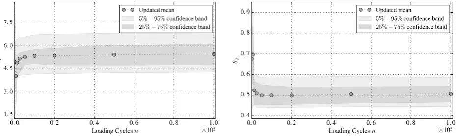
initial test runs and set to 5% of the 5th-95th inter-percentile range of the marginal priorsπ(θj). To reveal the sequential uncertainty reduction in the updated model parameters, the updated mean estimation of the jth component of θ, as well as its25% 75%,5% 95% uncertainty bands, are plotted against the loading cycles inFig. 3forj=1, 2, 3.

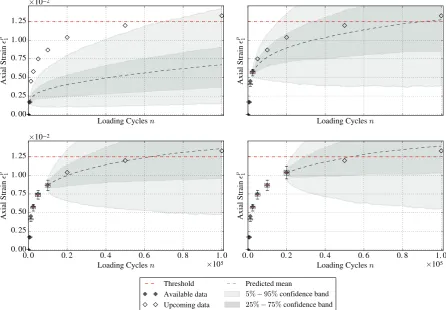
Next, based on the most up-to-date predictions of the permanent axial strain of the track,Algorithm 3is used for EOL and RUL calculation. To this end, the time-ahead predictions of the track settlement, which are depicted inFig. 2 using shaded areas to illustrate the prediction uncertainty, are extrapolated forward in time until the permanent axial strain crosses the threshold between the useful domain and the failure domain , whereby the PDF of EOL is obtained as a first-passage time distribution problem. For this example, the threshold is set to =0.0125 [di-mensionless], thus, the useful domain is defined as the subspace

={( , ) 2: = +1/3 [0, 1. 25·10 ] }

1 2 . To speed up

the EOL calculation, which requires the simulation ofN=5000 particle trajectories thousands (or even millions) of loading cycles ahead until reaching the failure domain, the ”natural” load cycles are converted toduty cyclesby dividing the load cycles by a fixed factorDC >1[40]. Here, a duty cycle is defined as an appropriate fixed amount of load cycles where a sensible amount of settlement is accumulated. After some pilot tests,

=

DC 50was revealed as a suitable value for this example.

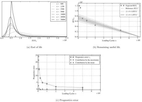
Fig. 4a shows the sequence of estimated PDFs of EOL for the dif-ferent load cycles when track settlement data are available. By com-paring between consecutive PDFs inFig. 4a, one can observe that the mean EOL prediction gradually tends to converge to the reference mean value for EOL* (blue marker inFig. 4a), and the prediction uncertainty (i.e., the spread of the PDFs) tends to decrease, as a consequence of the sequential updating of the model as long as new data are collected. The gradual increase in the prediction accuracy is also revealed inFig. 4b, where the mean RUL estimations are plotted against time of prediction using an accuracy cone type of representation[41]. Two cones of ac-curacy at 10% and 20% of the reference RUL, denoted here as RUL* and obtained as RUL*=EOL* n, are included to visually interpret the prognostics performance in regards to prediction accuracy. Observe that the expected RUL prediction is appreciably inaccurate for the in-itial 5000 load cycles (values out of accuracy cones), which suggests that a training stage is required by the model to learn from the data. This learning period is also manifested in Fig. 4c, where the proposed prognostics error nin Eq. (36) is plotted against loading

cycles assuming a Gaussian PDF centred at 75,000 and 10% c.o.v. for EOL*.

[image:10.595.38.561.79.114.2]

Finally, the prognostics performance of the track geometry de-gradation model proposed in Section 2 is compared with the Table 1

Permanent vertical strain data used for calculations. Data taken from[23]corresponding to ”RTF” test.

Loading cyclesn, ( × 103_{) 0 625 1250 2500 5000 10,000 20,000 50,000 75,000 100,000}

Plastic axial strain p

n

[image:10.595.39.287.655.744.2]

1 0 0.0017 0.0045 0.0058 0.0075 0.0087 0.0104 0.012 0.01275 0.0133

Table 2

Nominal values and prior uncertainty of model parameters and inputs used in calculations.

Type Parameter Value Prior PDF

Critical State Γ 2.99 Not applicable

M 1.9 Not applicable

λcs 0.194 Not applicable

κ 7·103 _{Not applicable}

Fitting (hardening model) α(θ1) – (1, 10)

β(θ2) – (0, 1)

performance of a well-known class of phenomenological models for track settlement [30,42,43], given by the logarithmic model

=A+Blog ,n

p

1 whereAandBare fitting parameters. For comparison

purposes, this model is referred to asmodel class 0, while the one proposed in Section 2is denoted asmodel class 1. A discrete-time state-space representation of model class 0 is obtained and

subse-quently embedded within the SIS particle filtering algorithm (refer to Algorithm 2), following the methodology inSection 3.1. For model class 0,the basic functions fnandgndefining the hidden Markov model are given byfn= 1pn 1+B n/ andgn= 1pn,respectively. The same uncertainty structure (i.e., modelling and measurement errors) that is assumed for model 1is also assumed for 0. The assessment

of the two model classes is carried out by computing the RPEnmetric proposed inSection 3.3. The results are shown inFig. 5for the load cycles where measurements are available. In view ofFig. 5, the physics-based model class 1proposed in this paper is revealed to be the one with the larger and earlier anticipation capability (RPEn> 1), since it provides larger RPEnvalues in the earlier stages of the process. More insight and discussion about prognostics performance is provided in the next section.

5. Discussion

5.1. On the case study results

The proposed methodology for knowledge-based prognostics for railway track degradation has been exemplified using the case study presented in the previous section based on data from the Nottingham Railway Test Facility. As a first interpretation of the results inFig. 2, the

proposed methodology is able to accurately anticipate the evolution of the plastic vertical strain of the track with quantified uncertainty after an initial learning stage using limited data. The length of such a learning stage is revealed inFig. 3, where the updated mean of the uncertain model parameters is shown to reach an asymptotic behaviour after the first 5000 load cycles (about 7% of the reference EOL*), which denotes that after this learning period the model has extracted enough information from the data to make accurate predictions. This is in agreement with the results shown inFig. 4b for the RUL estimations, and also with those inFig. 4c, wheren=5000is revealed as the time when the prognostics error measure n starts a slower and gradual

decrease; i.e., the predictions become increasingly accurate for cycles n> 5000, therefore making a decision based on the predicted EOLnis recommended from that time. Note also in Fig. 4c that the overall prognostics error n is mostly contributed by the uncertainty in the

[image:11.595.68.533.55.194.2]

(uncertain) value of the parameters[45]. This point is reinforced by the values RPEn> 1 inFig. 5, which reveals that the proposed physics-based model performs better predictions than the data-physics-based loga-rithmic model used as a benchmark (denoted as 0), needing less

support from the data to train the fitting parameters. This tendency is more accentuated in the earlier stages of the degradation process due to the initial lack of condition monitoring data. As the process evolves towards the end, both models have extracted enough information from the data to allow them to perform similarly.

In terms of the prediction uncertainty, observe fromFigs. 2and4a that the spread in the future predictions, which is initially high due to the high prior uncertainty in the model parameters (especially in the hardening parametersαandβ), tends to decrease as the model is se-quentially updated with new data, which is a common and desirable feature in any prognostics problem. However, it is also observed that the reduction of this prediction uncertainty does not take place gra-dually along the full extent of the process but concentrated at the initial stage, approximately coinciding with the learning period of the model where most of the data are available. In this respect, it should be pointed out that the observed uncertainty reduction is a particular consequence of the data collection pattern in this case study, i.e., col-lected over a set of non-regularly scheduled load cycles mostly con-centrated at the beginning of the process, and not a general feature of the proposed physics-based prognostics framework.

[image:12.595.69.530.59.391.2]

Besides the modelling uncertainties discussed above, there is an additional source of uncertainty coming from the prognostics algorithm itself, which is related to the asymptotic approach of the predicted plastic axial strain to the established threshold (as observed in Fig. 2). This asymptotic behaviour makes that many sample predictions need very long simulations to reach the threshold, which leads to poor EOL estimations unless the amount of particles (Nin Algorithm 2) is sufficiently large. A suitable solution to overcome this issue is by the adoption of dedicated prognostics algorithms based on high-efficiency sampling techniques, like the one recently proposed by the authors in[46]based on SubSet simulation, or the one developed by Yanet al. [47]based on adaptive Lebesgue sampling, among others. This task constitutes a desirable future improvement of this work.

[image:12.595.38.289.426.575.2]

Fig. 4.Results for track degradation prognostics. (For interpretation of the references to colour in this figure legend, the reader is referred to the web version of this article.)

Fig. 5.Relative prospective evidence (RPEn) obtained for the physics-based model class 1proposed inSection 2and an empirical logarithmic model class