Using real occupancy in retrofit decision-making:
Reducing the performance gap in low utilisation
higher education buildings
Stephen Oliver1*, Saleh, Seyedzadeh1, Farzad Pour Rahimian2 1 University of Strathclyde, Glasgow, UK
2 Northumbria University, Newcastle, UK * stephen.oliver@strath.ac.uk
Abstract
Retrofit analysis relies on intuition and faith in the simulations used to justify strategy selection. However, intuition is built upon belief systems which become increasing unjustifiable as building operation deviates from design whether in utilisation, occupant behaviours or climate models. Higher education facilities are known for persistently low but well recorded occupant presence and density, and therefore are susceptible to counterintuitive behaviours related to utilisation. When operation has little correlation with design it is possible for performance issues to appear to be symptoms of design considerations rather than direct root of the issue. Using an EnergyPlus and SBEM virtual case study based on a floor of a university building and class registration data this paper describes how lighting retrofit simulation alludes to intuitive thermal property and HVAC efficiency concerns where heating management is the primary cause for concern. In doing so, it demonstrates a new approach to scheduling utilisation in higher education facilities and a method of meaningfully modelling BMS systems in EnergyPlus as replacement for the efficiency credits method. Results are discussed in terms of relevance to legislative compliance, cost-benefit analysis and how the scheduling methods contribute to intuitive analysis of low utilisation buildings.
Keywords: Retrofit analysis, occupancy, compliance, low utilisation
1.
Introduction
Janda (2011) stated “buildings don’t use energy: people do” which is not entirely accurate. Building energy is in part consumed to meet the needs of people, but it is also attributable to the superstitions of the designer, building manager and occupants. Whether it is the designers’ assumption that operational utilisation will be comparable to design or occupants’ subjective perceptions, energy consumption can partially be attributed to misguided beliefs rather than needs. In the case of design assumptions, higher education facilities’ utilisation of teaching spaces in the UK is recorded is typically around 27% (Space Management Group, 2008) which is neither represented in compliance models nor meaningfully accommodated by existing utilities, despite utilisation being considered a primary cause of the building performance gap (Hong et al., 2016; Kneifel et al., 2016; Ridley et al., 2014). Occupant behaviours inherently have significant impact on net energy demand and the occupants collective comfort (Guerra-Santin et al., 2016; Liisberg et al., 2016; Tagliabue et al., 2016; Yousefi et al., 2017) but even those behaviours are bound to superstitions. Personality traits (Schweiker et al., 2016), internal rendering colours (Wang et al., 2018), perception of environmental control (Schweiker and Wagner, 2016; Yun, 2018) and even hearing another occupant describe temperature (Wang et al., 2018) citing (Höppe, 2002) affects occupants’ beliefs about the ecosystem they reside.
Heating is an ecosystem-sensitive consumer in the sense changing the operational state of any discrete space within a building affects the heating of the remaining spaces. Given energy performance policy and plans to decarbonise the grid, heating perhaps deserves special attention despite UK compliance focus on carbon emissions. Intuition suggests the solution is to throw money at improving envelope and/or heating, ventilation and air conditioning (HVAC) system performance however; the former is not suitable for discrete spaces and both are based upon the belief that high heating energy is an illness rather than, say, needles exertion or overexertion of the HVAC.
Previous works identify sensitivity to occupant behaviours (Corgnati et al., 2017), climate (Rastogi, 2016) and underutilisation (Gupta and Gregg, 2016) which ultimately highlight it is not helpful to think of retrofit analysis as a means of consistently identifying optimal solutions. Instead attempting to frequently to select economically viable, better than no action solutions. Rastogi offers a methodology for generating synthetic weather data for assessing retrofits and designs under probable climates. Lee et al. (2018) discuss a complementary Monte Carlo-based risk aversion method which mitigate some superstitions. Are nonetheless susceptible to the in-built deviation in the building energy model. Gupta and Gregg (2016)identified a similar mismanagement hypothesis as discussed in this paper suggesting manual intervention from staff or some level of local smart radiator controls though they were not able to test the hypothesis. In a similar theme, this paper simulates lighting retrofits using explicitly known utilisation under two climates with and without heating management to frame resulting high heating demand as a symptom of needless exertion of the HVAC rather than of poor envelope and boiler performance.
2.
Methodology
Using a bespoke building model interfacing library, it aims to demonstrate the exploitability and necessity of using class registration data during retrofit analysis. The subsection of the research covered in this paper discusses the effects of real-world scheduling on simulated energy demand in relation to compliance- and operational savings-led decision-making using the results of 100 EnergyPlus and 19 SBEM (Simplified Building Energy Model) simulations. Once utilisation’s significance for the case study has been established, a case is built for introducing a heating management system (HMS) as a precursor to decision-making. A novel approach to meaningfully modelling the HMS is proposed which remedies the shortfalls of the efficiency credits method offered by the building regulations.
2.1.
Virtual case study
2.2.
scheduling
Three standard schedule scenarios and two complementary building management system supported for non-NCM scenarios were created which represent the building’s operations with the real-world utilisation. Presence and density is taken from the class registration system.
NCM: A collection of standard schedules used for design and compliance modelling. These assume consistent presence across every standard weekday with separate near-zero utilisation schedules for weekends and holidays. The schedules are ignorant of the real building and year but are susceptible to change with revisions of the NCM.
Explicit/Implicit: Where registration data is available for a teaching space custom utilisation and lighting schedules are created. Utilisation during occupied periods is defined separately for each registered period based on the registration system’s definition of the zone’s capacity and the number of occupants registered for the class. Lighting is defined as Boolean-state based on the presence state from the registration system. Where a zone has registered periods with zero occupant density the zone is considered reserved with zero density. Finally, explicit scheduling assumes that a teaching space with zero entries in the registration system is unknown and assumed to be worst case using the appropriate NCM schedule. The Implicit scenario assumes that the registration system is complete and therefore any teaching space which has no entries in the system is never utilised during schedule year.
Explicit- / Implicit-BMS: Extending the Explicit and Implicit schedules, the rules applied to create the scenarios are used to define BMS system configuration. The data from the registration system used to generate each teaching space’s utilisation and lighting schedules are used to convince EnergyPlus that a BMS is installed for the spaces by toggling the heating source accessibility. A preheat period is added to each presence period at one hour as per the default assumption.
2.3.
Lighting design and BMS cost methods
Costing methods for lighting and BMS installation were created through reference to a lecture from Philadelphia University and price estimates from the SPON’s 2018 Mechanical and Electrical Services Price Book 2018.
2.4.
Lighting (R-LIG)
The lighting retrofit cost method uses the photometrical computation (Lumens method) method documented in the Philadelphia University Electrical Installation lecture 11 The method uses photometric data to estimate the number of luminaires required to light a given environment through lookup using the room index (k), a simple function of a zone’s geometry. Given as:
2.5.
Building management system (R-BMS)
Being a computerized system attached to local control measures, the heating management system method is a function of the number of registered zones. The method was reduced to two primary costs, Head Equipment priced at £15,000 and Intelligent Unitary Controllers at £500/IUC. Cost method is given as:
C = Total cost of installation in £, Hc = Global cost for head end equipment (software, computer, commissioning) in £, I = Unit cost for each intelligent unitary controller £, N = Number of IUCs.
2.6.
Results
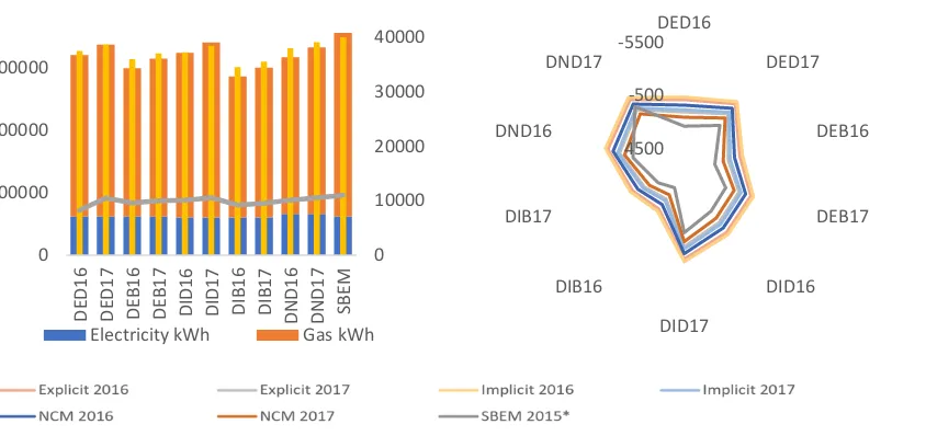
Figure 1 & 2: Estimated annual running cost (right y), consumption and emissions (left y) by Schedule-Climate / engine, and Schedule-Schedule-Climate scenario running cost disparity. Labels represent strategy and year <lightis>-<schedule>-<BMS>-<year> where (D)efault, (E)xplicit, (I)mplicit, (N)CM, and (B)MS Using NCM as design utilisation, Explicit scheduling results in a reduction of 52% in presence hours for the teaching spaces and Implicit resulting a reduction of 86%. Figures 1 and 2 show the base model annual net energy demand for each Schedule and Climate (Schedule-Climate) scenario and how they compare to one another. Notably, Explicit- / Implicit hold the highest and lowest annual consumption dependent on whether teaching space heating is managed.
2.7.
Schedule presence
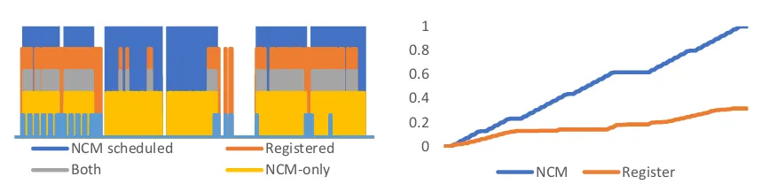
Figures 3 and 4 show difference between NCM and registration system presence demonstrate the disparity cumulative presence and overlap between the NCM and registration system schedules for zone GH818 which has the second highest presence hours and the greatest overlap between NCM and Explicit schedule. There is no cooling in this building however, it is worth noting utilisation during the cooling period is significantly lower than in NCM.
807 813 816 817 818 863 898 801A* 801B* 801C* 801D* 801E* 801F*
0 10000 20000 30000 40000
0 200000 400000 600000
DE
D16
DE
D17
DE
B16
DE
B17
DID16 DID17 DIB16 DIB17 DND16 DND17 SBE
M
Electricity kWh Gas kWh
-5500
-500
4500 DED16
DED17
DEB16
DEB17
DID16
DID17 DIB16
DIB17 DND16
[image:4.612.79.501.243.442.2]NCM 2,134 2,134 2,134 2,134 2,134 2,134 2,134 2,134 2,134 2,134 2,134 2,134 2,134 Explicit --- 745 639 611 633 483 675 2,134 2,134 2,134 2,134 2,134 2,134 Implicit --- 745 639 611 633 483 675 --- --- --- --- --- --- %-Imp 0.00% 34.91% 29.92% 28.61% 29.66% 22.63% 31.61% 0.00% 0.00% 0.00% 0.00% 0.00% 0.00%
Table 1: Teaching space presence hours by Schedule
Figure 3: Schedule scenario overlap GH818. Figure 4: Cumulative presence GH818
2.8.
Schedules, lighting and net building energy demand
Table 1 shows annual lighting electricity consumption for teaching spaces under each Schedule. NCM scheduled teaching spaces contribute 20% of the total lighting demand equivalent to 10% of the buildings annual grid-supplied electricity demand. However, with registration system presence and implied absence their contribution is reduced to 10% and 3.6% for Explicit and Implicit scenarios respectively. In absolute terms, these changes reduced grid-supplied electricity demand by 6.8MWh and 10.8MWh for Explicit and Implicit, respectively. Conversely, absence of internal gains from assumed presence increased natural gas demand for heating by 14.5MWh and 25.1MWh for 2106 and 15.2MWh to 27.3MWh for 2017 with Explicit-/Implicit-2016 against NCM-2016 and Explicit- / Implicit-2017 against NCM-2017, respectively. The heating rise is explained primarily by the absence of heating system management resulting in extra demand to maintain zone temperature where free gains from lighting and latent gains from occupants are not present.
The relationship between lighting and simulated natural gas demand is not easily expressed due to the temporal, seasonal, utilisation (presence, density, humidity changes), external gains and latent value of each Watt internal gains. Nonetheless, even if adjacency awareness in the simulation engine is ignored each Wh of electricity consumed by lighting is worth more than its cost in terms of net energy demand. Considering NCM-2016 compared to Explicit-2016 and Implicit-2016, internal gains from occupants and lighting change by 17.5MWh and 28.9MWh, respectively. The scenario changes’ impact on annual gas consumption whilst not entirely comparable can be used to estimate that the monetary value of each Wh electricity that would have been consumed by lighting with each Wh lighting contributing 23.8% and 23.3% of the cost of every Wh net energy demand increase. However, this is only 21.3% during the academic year. Factoring latent and lighting gains with the existing lighting system into the increase in net energy demand reduces the value of each kWh saved from lighting consumption to 50% and 46% for Explicit-2016 and Implicit-2016 against NCM-Implicit-2016. In contrast, Implicit-Implicit-2016’s Wh/Wh rate retains 3.1% above 1:1 where heating is managed. In summary, lighting consumption and net energy demand do not have a 1:1 relationship. Under design conditions this means each Wh lighting is worth 1Wh of electricity and a fraction of 1Wh of the heating demand, in the case of this building 1.84Wh. Therefore, under design utilisation each Wh of lighting reduces emissions 0.181gCO2/Wh and £0.00003/Wh reducing its effective unit cost to £0.1253/kWh.
Whereas, Implicit-2016’s lighting consumption reduction of 10.6MWh electricity, increases heating demand by 2.53MWh, nullifying 0.3tCO2 of the electricity related emissions reduction and increasing the
NCM scheduled Registered
Both NCM-only
0 0.2 0.4 0.6 0.8 1
£/kWh cost of the new gas consumption from £0.0358/kWh to £0.044/kWh offsetting 15% of £/kWh saved from the schedule change.
[image:6.612.84.531.115.251.2]2.9.
Lighting retrofit
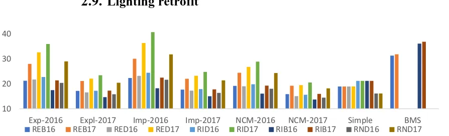
Figure 5: Schedule-Climate scenario relative discounted payback periods at 3.5%
Figure 5 shows the lighting retrofit for the virtual case study in terms of discounted payback period based on the difference between the base model simulated annual running of the x-axis and the savings from the bar labels Schedule-Climate scenarios. Additionally, BMS represents heating managed compared to heating managed and simple representing where dependent consumer fuel consumption changes are ignored. As with discussion in 4.2, the discounted payback period is volatile depending on the chosen Schedule-Climate scenario for the base model and the scenario assumed to produce the closest approximation of the annual run cost savings. Most SBEM results never return on the capital investment with NCM-2017, NCM-2016 and Explicit-2017 paying back after 24,8, 34.8 and 37.9 years. Across all scenarios where an HMS is not included in the base model estimated running cost, the ranges of disparity span 65% to 162%. SBEM excluding one result at 55 years has a maximum disparity of 190%. In contrast, disparity ranges between 46% and 88% at the bank base rate. However, where HMS is presented the disparity range is only 18%. The suggested 7% private project rate has significant implication for results where 38 Schedule-Climate scenarios entirely fail to payback in contrast to 3.5%. The lighting retrofit for bars labels as “D” for the BMS flag are calculated based on the lighting capital cost £83,112 whereas each with “B” for the flag include £21,500 for the BMS system with a total cost of £104,612. Despite the extra 26% cost the payback period for all heating managed comparisons not compared to the heating managed base model estimate a payback period of lower than any other Schedule-Climate of without management. A key feature of the BMS group is that using the BSCG efficiency credits method of representing a BMS would not payback even though the cost used is ignorant of 66 zones and the credits gained would be applied all zones served by the LTHW boiler. Furthermore, the efficiency credits method would overestimate gas contribution to annual running cost by £3,000 to £3,300 for Implicit 2016- and 2017-HMS respectively.
10 20 30 40
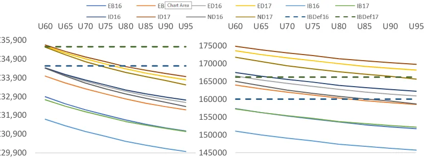
Figure 6: Annual running cost post-retrofit all lighting constant efficacy upgrades at the number of on the x-axis label in lm/cW. Series names represent Schedule-BMS-Year
Figure 7: Annual kgCO2 post-retrofit for each retrofit with baseline 2016 / 2017 HMS.
Running costs although improving over each retrofit scenario support previous discussion on managed and unmanaged heating in low utilisation areas. First, proportional to the utilisation, the costs of unmanaged are greater than NCM scheduled running costs. Compared to NCM savings as efficacy increases, lower utilisation result diverges from NCM savings diminishing in return. In contrast, managed heating results in significantly lower running cost and becomes increasingly proportional to NCM scenarios as efficacy increases. Carbon emissions are more interesting. Ignoring the inherent benefit of an HMS as noted elsewhere, retrofitting the lighting without an HMS results in simulated NCM performance suggesting that performance and running cost improvements would be better despite 96.5% greater lighting utilisation in teaching spaces with NCM schedules. This observation is likely the key contribution of this paper given this would not be identifiable without the BMS modelling method used in this paper Horizontal lines represent HMS baseline running cost and carbon emissions. Estimating from SPON’s default LED luminaire and labour cost, to achieve those lines through lighting retrofit requires three times the cost of the HMS for a fully qualified HMS. Though not discussed in this paper, a rudimentary HMS could ostensibly be installed for less than £1,000 using smart radiator valve controllers.
4.
Discussions
More often than not it is either not possible to meter a discrete space or there is no metering available which means there is rarely a meaningful opportunity to use operational data unless servicing is homogenous, and the discrete space represents a significant portion of the total gross internal area.
4.1.
Heating management
It is clear from all dynamic simulations where Schedule-Climate scenarios are considered that in the case of the virtual case study, low utilisation is detrimental to heating demand resulting in volatile effects on the net energy demand. Lighting demand was reduced by 8.3% and heating demand increased by 5.0%~ for both 2016 and 2017. However, these resulted in different changes across the four metrics, net energy demand, running cost, carbon emissions and cost per emission kilogram CO2 for all Schedule-Climate scenarios. Net energy demand increased and running cost decreased for all Schedule-Climate scenarios though not proportionally but, kgCO2/m² values did not behave intuitively. Where a simple estimation based on efficacy may have been used the change from NCM to Implicit would be expected to return 1.97
£29,900 £30,900 £31,900 £32,900 £33,900 £34,900 £35,900
U60 U65 U70 U75 U80 U85 U90 U95
145000 150000 155000 160000 165000 170000 175000
kgCO2/m² difference however, the offset from heating demand increase reduced this to 0.07kgCO2/m² for 2016 and increased 2017 by 0.09 kgCO2/m². The results are further compounded when kgCO2/£ is considered, the suggested metric for equiproportionate abatement where a lower value shows greater potential for compliance-oriented application. NCM 2016 surprisingly suggests greater opportunity than NCM-2017, and Implicit-2017 less opportunity than Implicit-2016.
Heating management resulted in significant improvements across all metrics including up to 6kgCO2/m² from NCM to Implicit and the expected NCM > Explicit > Implicit relationship was now realised. This was not exclusive to emissions, the abatement metric now favoured Implicit and NCM and Explicit were on par. This translated over to lighting as well where although the initial 1.84Wh lighting net energy value was reduced to 0.5Wh and 0.46Wh without HMS in teaching spaces for Explicit and Implicit respectively, with the HMS the net energy value improved to 1.03Wh. The case study has no comfort cooling and the absence during the summer as highlighted in Figure 3 would significantly reduce cooling load. Nonetheless, GH818 at least is almost never occupied during the cooling period and therefore its cooling demand would be all but wasteful. Though, it is worth noting that all teaching spaces which are not GH801* have NCM scheduled adjacencies whose cooling demand would likewise be reduced. The virtual case study did make accommodation for adjacent floors to mitigate heat loss miscalculation however, the principle of scheduling lower utilisation will only further be skewed as other floors are calibrated.
Without an HMS the virtual case study suffers from reduction in internal gains to the point where for some metrics the 70%~ reduction of presence hours for 23% of the building becomes negligible. Since this building is served by natural gas, the problem would only increase with any other non-renewable fuel.n. Without management Schedule-Climate scenarios behave unpredictably and lighting waste heat’s value is around double. Failure to manage dependent consumers make performance and results volatile across all metrics and may convince consultants that symptoms of its absence are design failures rather than operational.
4.1.1.
Heating management and compliance
BMS simulation for compliance is not well-defined due to the absence of persistent scheduling data.. The compromise for implementing HVAC control measures is to increase the CoP of heating systems as per the system relevant allowance from the Building Services Compliance Guide. In the case of the virtual case study LTHW boiler, this is an increase of 4% for a full BMS in lieu of a heating-only option. The improvement from this is insignificant. SBEM’s original heating demand was 198.94kWh/m² compared to 175.13kWh/m² to 186.14kWh/m², 183.89kWh/m² to 195.65kWh/m² for NCM-2016 and NCM-2017, and Implicit-2016 and Implicit-2017 respectively. Using SBEM as a proxy for the efficiency credits method the improvement only improves heating demand by 7.68kWh/m² or £789/annum. The efficiency credits method is priced on the entire discrete which would cost £46,000. Even using the MEES DPP rate of 0.75% the efficiency credits method would take 77 years to payback.
4.2.
Lighting retrofit
The simple calculation bracket presented in section 3.3 serves two purposes 1) it shows how Schedule scenario affects the payback period with a 26% increase despite teaching spaces only representing 23% of gross internal area. 2) The results demonstrate the estimations simple online tools claiming suitability for nondomestic buildings such as those provided by Emerson, Spirit or Regency Lighting are increasingly inappropriate as utilisation decreases. These values are not necessarily wholly spurious if the building is notably better insulated and has high utilisation which is evident from the discussion in section 3.2 noting 79% to 76% of gains lost through absence in Schedule scenarios are associated with latent gains from occupants.
Each of the standard six Schedule-Climate scenarios compared to all eleven including SBEM results are highly disparate with the entire set having a disparity range between 48% and 190%. This is obviously not reliable, excluding comparisons between NCM-2016 and NCM-2017 which is 20% to 41% at 3.5%. NCM highlights sensitivity to climate though at the bank base rate the payback period is only 2 year longer for 2016/2017 to 2017. However, HMS introduced to non-NCM Schedule-Climate scenarios based on their counterpart managed base model have a maximum disparity of 18% at 3.5% and only 10% at the bank base rate. This may be attributed to the significantly reduced fuel demand and retained greater than 1:1 lighting consumption to net energy demand ratio associated with proper management of the teaching spaces. It was to be expected that heating management would reduce the volatility of heating demand however, it was not expected to have as significant mitigating effects on Climate The difference in base model heating demand between Implicit and Implicit-HMS ranged from 81,200kWh and 109,800kWh for 2016 and 2017.These results show why dependent consumer management is not just relevant to mitigating counterintuitive behaviours from retrofitting independent consumers when real utilisation significantly deviations from design. They also appear to reduce uncertainty attributed to climate almost proportionally to the difference in design and real utilisation with managed heating.
Constant efficacy retrofit simulations demonstrate that although estimated running costs decrease in all scenarios, energy performance across both emissions and net energy performance metrics. That is, not only would the savings and subsequent cost-benefit analysis results be skewed by NCM over real utilisation schedules, implementing any of the eight full building lighting retrofits without managed heating would result in poorer performance than design utilisation, including running cost. It is universally more expensive to operate the building without management than it is to operate at design utilisation post-retrofit. In terms of Part L2A, this may result in a pass that is underserved. MEES would be a legal, practical and economic nightmare. Where heating is unmanaged, it may receive an undue exemption from upgrade requirements and the decision-making process may lead to selection strategies damaging or at least ineffective to the real world. It’s hot topic the extent which compliance-led retrofits need to align before liability is a legal concern, but it is not through lack of discussion. In terms of ESOS-2019 which is bound to operation net energy demand, the negative impact of increased demand would not be apparent until 2023 when updated reports are required. Finally, with the electrification of the grid ambitions, ignoring heating heat management would be detrimental to long-term targets. All-in, retrofitting lighting in low utilisation areas without first implementing heating management is possibly the worst decision available for the virtual case study despite being lauded as an easy and safe win.
4.3.
Implication for ESOS-, Part L2B- and Section 63-led retrofitting
assumption of business as usual having a net present value of £10,133 or £8,931 more than expected over 7 years at 3.5% and 7% respectively. This would also be the difference between lighting appearing as 41% to 61% of a Scottish EPC band rather than 7% to 12%, or 11% and 65% of an English EPC band – against the current SER. ESOS prior to considering retrofitting, however, would perhaps be more concerning since without some correlation between the reported operational and simulated fuel demands, calibration is untenable.
In terms of MEES for England, Wales and Northern Ireland, the difference in lighting energy consumption is nearly equivalent to paying for the lighting retrofit costs associated with the teaching zones alone less than 3 years outwith the 7-year retrofit measure exemption cut off. Using constant efficacy retrofit simulations it was shown that unmanaged heating in low utilisation spaces not only resulted in higher running cost estimates than of design utilisation despite 86% lower presence hours in registered spaces, but retrofitting causes the building to perform worse than estimated for design utilisation. This is not necessarily an explicit concern for decisions made purely for MEES or Section 63 compliance, after all meeting compliance is about cheating the simulation model first and reducing emissions second, but it certainly won’t help the reputation of consultants. ESOS and retrofit-as-service are critically damaged by retrofitting without an HMS and electrification of the grid ambitions add insult to injury. In terms of policy and as a service decision-making, lighting on its own is unadvisable by any metric.
None of the Schedule-Climate scenario comparisons are within the 7-year MEES exemption and therefore the lighting retrofit would not need to be applied or considered as part of a strategy package. However,, it does reduce carbon emissions by 13% to 17% for NCM and Implicit-BMS scenarios comparisons respectively where the base Schedule-Climate and retrofit Schedule-Climate scenarios are based on the same Schedule scenario and climate year. Although not part of this paper, it was estimated that were a boiler replacement retrofit included with the R-LIG + R-BMS package and priced using SPON’s, the retrofit package payback period would decrease from 32 to 26 years for the lower bound estimate.
5.
Conclusion
Design and low utilisation simulated energy performance across monetary, emissions and net energy metrics have a spurious relationship. While with some general understanding of the utilisation one may be able to use intuition to estimate how the relationship between independent on dependent consumers may affect net energy demand and possibly to annual running costs to an extent. However, the relationship when considering Schedule-Climate and engine across all metrics is far from predictable. Though teaching spaces occupied less than 25% of the building, scheduling using registration data had profound effects on the simulation engines’ analysis of the building. It is informally known that utilisation persists around 30% throughout the building, though not registered meaningfully, were all areas suitably registered the negative impact would be significantly worse.
modelling enabling meaningful calibration with the utilisation-calibrated model. Finally, the HMS was three times cheaper than the SPON’s estimate for the constant efficacy R-LIG to achieve at least the same running cost improvement as unmanaged heating 60lm/cW against 2017 climate and all unmanaged or design schedules emissions reduction until 85lm/cW against 2016.
Scheduling reduced lighting consumption in the associated zones to the point where estimating the payback period exclusively on lighting energy consumption still resulted in payback periods longer than luminaire lifecyle even at the bank base rate used for MEES compliance. When considering net energy demand without an HMS the results were three and a half times greater than MEES exemption criteria at the bank base rate and well outwith the luminaire lifecycle for the public project discount rate. However, with heating management installed purely in the registered spaces with Implicit- scenarios were the worst case just over twice the exemption period. All teaching spaces bar one under Implicit- scenarios do not run long enough for LEDs to have merit. Therefore, T5s for teaching spaces may be a more suitable solution.
Retrofit analysis relies on intuition whose origin verges on superstition though it is understandable given reliable modelling of real-world unmanaged heating has not been demonstrated in the literature and stochastic modelling would not account for the variations in teaching space utilisation. Intuition suggests envelope or heating HVAC efficiency are primary concerns however, clearly these mitigate the symptoms not the cause.
Acknowledgements: The research presented in this paper would not be possible without the considerable support from arbnco Ltd in both funding the corresponding author’s MPhil and supporting their professional development over the last decade.
References
Chaudry, M., Abeysekera, M., Hosseini, S. H. R., Jenkins, N., & Wu, J. (2015). Uncertainties in decarbonising heat in the UK. Energy Policy, 87(Supplement C), 623-640. doi:https://doi.org/10.1016/j.enpol.2015.07.019
Corgnati, S. P., Cotana, F., D’Oca, S., Pisello, A. L., & Rosso, F. (2017). Chapter 8 - A Cost-Effective Human-Based Energy-Retrofitting Approach. In F. Pacheco-Torgal, C.-G. Granqvist, B. P. Jelle, G. P. Vanoli, N. Bianco, & J. Kurnitski (Eds.), Cost-Effective Energy Efficient Building Retrofitting (pp. 219-255): Woodhead Publishing.
Guerra-Santin, O., Romero Herrera, N., Cuerda, E., & Keyson, D. (2016). Mixed methods approach to determine occupants’ behaviour – Analysis of two case studies. Energy and Buildings, 130, 546-566. doi:10.1016/j.enbuild.2016.08.084
Gupta, R., & Gregg, M. (2016). Empirical evaluation of the energy and environmental performance of a sustainably-designed but under-utilised institutional building in the UK. Energy and Buildings, 128, 68-80. doi:https://doi.org/10.1016/j.enbuild.2016.06.081
Hong, T., Sun, H., Chen, Y., Taylor-Lange, S. C., & Yan, D. (2016). An occupant behavior modeling tool for co-simulation. Energy and Buildings, 117, 272-281. doi:10.1016/j.enbuild.2015.10.033 Höppe, P. (2002). Different aspects of assessing indoor and outdoor thermal comfort. Energy and Buildings,
34(6), 661-665. doi:https://doi.org/10.1016/S0378-7788(02)00017-8
Janda, K. B. (2011). Buildings don't use energy: people do. Architectural Science Review, 54(1), 15-22. doi:10.3763/asre.2009.0050
Lee, J., McCuskey Shepley, M., & Choi, J. (2019). Exploring the effects of a building retrofit to improve energy performance and sustainability: A case study of Korean public buildings. Journal of Building Engineering, 100822. doi:https://doi.org/10.1016/j.jobe.2019.100822
Lee, P., Lam, P. T. I., & Lee, W. L. (2018). Performance risks of lighting retrofit in Energy Performance Contracting projects. Energy for Sustainable Development, 45, 219-229. doi:https://doi.org/10.1016/j.esd.2018.07.004
Liisberg, J., Møller, J. K., Bloem, H., Cipriano, J., Mor, G., & Madsen, H. (2016). Hidden Markov Models for indirect classification of occupant behaviour. Sustainable Cities and Society, 27, 83-98. doi:10.1016/j.scs.2016.07.001
Pomponi, F., Farr, E. R., Piroozfar, P., & Gates, J. R. (2015). Façade refurbishment of existing office buildings: Do conventional energy-saving interventions always work? Journal of Building Engineering, 3, 135-143.
Rastogi, P. (2016). On the sensitivity of buildings to climatethe interaction of weather and building envelopes in determining future building energy consumption. EPFL, Retrieved from
http://infoscience.epfl.ch/record/220971/files/EPFL_TH6881.pdf
Ridley, I., Bere, J., Clarke, A., Schwartz, Y., & Farr, A. (2014). The side by side in use monitored performance of two passive and low carbon Welsh houses. Energy and Buildings, 82(Supplement C), 13-26. doi:https://doi.org/10.1016/j.enbuild.2014.06.038
Schweiker, M., Hawighorst, M., & Wagner, A. (2016). The influence of personality traits on occupant
behavioural patterns. Energy and Buildings, 131, 63-75.
doi:https://doi.org/10.1016/j.enbuild.2016.09.019
Schweiker, M., & Wagner, A. (2016). The effect of occupancy on perceived control, neutral temperature, and behavioral patterns. Energy and Buildings, 117, 246-259. doi:10.1016/j.enbuild.2015.10.051 Space Management Group. (2008). UK Higher Education Space Management Project - Evaulation. Tagliabue, L. C., Manfren, M., Ciribini, A. L. C., & De Angelis, E. (2016). Probabilistic behavioural
modeling in building performance simulation—The Brescia eLUX lab. Energy and Buildings, 128, 119-131. doi:10.1016/j.enbuild.2016.06.083
Wang, H., Liu, G., Hu, S., & Liu, C. (2018). Experimental investigation about thermal effect of colour on thermal sensation and comfort. Energy and Buildings, 173, 710-718. doi:https://doi.org/10.1016/j.enbuild.2018.06.008
Yousefi, F., Gholipour, Y., & Yan, W. (2017). A study of the impact of occupant behaviors on energy performance of building envelopes using occupants’ data. Energy and Buildings, 148, 182-198. doi:10.1016/j.enbuild.2017.04.085