Distributed current sensing technology for protection and fault location applications in HVDC networks

Distributed Current Sensing Technology for protection and Fault Location

Applications in HVDC networks

Dimitrios Tzelepis†, Adam Dy´sko†, Campbell Booth†, Grzegorz Fusiek†, Pawel Niewczas†, Tzu Chief Peng† †_{Department of Electronic & Electrical Engineering, University of Strathclyde, Glasgow, UK}

[email protected], [email protected], [email protected] [email protected], [email protected], [email protected]

Keywords—Multi terminal direct Current, Differential protec-tion, Travelling waves, Distributed sensing

Abstract

This paper presents a novel concept for a distributed current optical sensing network, suitable for protection and fault location applications in High Voltage Multi-terminal Direct Current (HV-MTDC) networks. By utilising hybrid Fibre Bragg Grating (FBG)-based voltage and current sensors, a network of current measuring devices can be realised which can be installed on an HV-MTDC network. Such distributed optical sensing network forms a basis for the proposed ‘single ended differential protection’ scheme. The sensing network is also a very powerful tool to implement a travelling-wave-based fault locator on hybrid transmission lines, including multiple segments of cables and overhead lines. The pro-posed approach facilitates a unique technical solution for both fast and discriminative DC protection, and accurate fault location, and thus, could significantly accelerate the practical feasibility of HV-MTDC grids. Transient simulation-based studies presented in the paper demonstrate that by adopting such sensing technology, stability, sensitivity, speed of oper-ation and accuracy of the proposed (and potentially others) protection and fault location schemes can be enhanced. Fi-nally, the practical feasibility and performance of the current optical sensing system has been assessed through hardware-in-the-loop testing.

1. Introduction

Power transmission based on High Voltage Direct Current (HVDC) networks is expected to be the favoured technology for massive integration of renewable energy sources and the realisation of European and Asian supergrids [1], [2]. DC-side faults are the greatest challenge when it comes to the realisation of HVDC-based grids, due to the fact that large inrush currents escalating over a short period of time [3].

After the occurrence of a DC-side fault on a HVDC trans-mission system, dedicated protection schemes are expected to minimise its adverse effects, by initiating fault-clearing actions such as selective tripping of circuit breakers. Follow-ing the fast and successful fault clearance, the next important action is the accurate calculation of its distance with regards to feeder’s length. This is of major importance as it will permit faster system restoration, diminish the power outage time, and therefore enhance the overall reliability of the system.

Distributed sensing in power systems is an advanced, cutting-edge technology (with numerous operational, technical and

economic benefits) which aims to accelerate power system protection and control applications [4]–[11]. In this paper the work conducted in [4], [5] is further demonstrated to highlight the technical merits when adopted for protection and fault location applications in HVDC networks.

2. Modelling

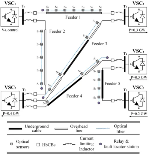
For the studies presented in this paper, a five terminal Multi-Terminal Direct Current MTDC grid (illustrated in Figure 1) has been developed in Matlab/Simulink. The system architec-ture has been adopted from the Twenties Project case study on DC grids. There are five 400-level, Modular Multilevel Converters (MMCs) operating at ±400 kV (in symmetric monopole configuration), Hybrid Circuit Breakers (HbCBs), and current limiting inductors at each transmission line end.

Figure 1: Five terminal MTDC grid.

at junctions and feeder terminals. The measurements are captured and processed at each line terminal (‘relay & fault locator station’). Transmission lines have been modelled by adopting distributed parameter model, while for the DC breaker a hybrid design by ABB [12] has been considered. The parameters of the AC/DC network components are de-scribed in detail in Table 1 and line parameters in Table 2.

TABLE 1: MTDC network parameters.

Parameter Value

DC voltage [kV] ±400

DC inductor [mH] 150

AC frequency [Hz] 50

AC short circuit level [GVA] 40

AC voltage [kV] 400

TABLE 2: Lengths of OHLs and UGCs Included in MTDC Case Study Grid.

HTM-1 OHL: 180 km

HTM-2 OHL: 120 km

HTM-3 OHL-a: 65 km, UGC: 180 km, OHL-b: 35 km

HTM-4 UGC: 50 km, OHL: 130 km

HTM-5 UGC: 90 km

3. Single-ended differential protection scheme

3.1. Protection algorithm

The single-ended differential protection algorithm is illus-trated using a flowchart in Figure 2 [4].

Figure 2: Protection algorithm of single-ended differential protection scheme.

Using the measurements of two consecutive sensors, the algorithm starts by calculating a series of differential currents given by

∆i(f)(t) =is(f)(t−∆t)−is(f+1)(t) (1)

where∆i(f)(t)is the f-th differential current derived using

the currentsis(f),is(f+1) measured at two adjacent sensors

f and f + 1 respectively (f = 1,2, ..., n−1) and ∆t the amount of time compensation due to propagation delays.

The protection logic has three stages. The first stage (Stage

A) is a comparison of differential current ∆i(f)(t) with a

predefined threshold value IT H. When the threshold IT H is exceeded for a differential current ∆i(f), the protection

algorithm will inspect the historical data of dis(f)/dt and

dis(f+1)/dtusing a short time window∆tw= 0.2ms. If any of the historical values of the derivativesdis(f)/dt(t−∆tw) or dis(f+1)/dt(t − ∆tw) exceed a predefined threshold

di/dt_{T H}, the criterion for StageBis fulfilled. This stage will ensure stability of protection to any kind of short disturbance. The final stage (Stage C) is included to ensure that the operation of the protection scheme does not originate from any sensor failure. If no sensor failure is detected, Stage C initiates a tripping signal to the corresponding CB.

The resulting key advantages of the proposed single-ended differential protection include high speed of operation, en-hanced reliability and superior stability. Detailed evaluation of the method can be found in [4].

3.2. Simulation results

The protection performance of the proposed scheme has been tested for numerous faults along the MTDC case study grid (fault have been applied on Feeders1,2and5). It should be noted that the protection scheme is based on a sampling rate of 5 kHz.

0 2 4 6 8

Idiff

[kA]

I

diff(S1-S2)

I_diff(S2-S3)

I_diff(S3-S4)

I

diff(S4-S5)

I

diff(S5-S6)

I

diff(S6-S7) Trip CB₁

(a) Differential current∆i(f)(t).

-2 0 1 2 3

dI

DC

/dt [MA/s]

S

2

S

3 Trip CB

1

(b) Rate of change of DC current.

0 2 4 6 8

IDC

[kA]

Nominal path Commutation branch Surge arrester Trip CB

1

tCB= 2ms

(c) Fault current interruption in HbCB.

100 101 102 103 104 105 106 107

Time [ms]

0 2 4 6 8

IDC

[kA]

Nominal path Commutation branch Surge arrester Trip CB₂

tCB= 2ms

(d) Experimental setup diagram.

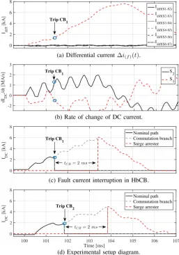
Figure 3: Illustration of pole-to-pole fault at Feeder 1.

terminal T1) on Feeder 1. This fault is practically located

between sensorsS2andS3. As such, the differential current

Idif f(S2−S3) calculated from the measurements of sensors

S2 and S3 is increasing rapidly (Figure3a), exceeding the

protection threshold, and hence, fulfilling Stage A. Figure 3b demonstrates that prior to the fault detection the rate of changediDC/dtfor both currents (sensorsS2andS3) is

non-zero which indicates the fulfilment of Stage B. A tripping signal is initiated by the third criterion (Stage C), however it is not depicted here due to space limitations. The fault current interruption is depicted in Figure 3c and Figure 3d for both ends of Feeder1.

The summarised results are presented in Tables 3 and 4 for pole-to-pole and pole-to-ground faults (with ground fault re-sistances of up to 300Ω) respectively. It can be demonstrated that in all cases only the required breakers operate, proving high selectivity of the scheme.

TABLE 3: Protection performance results for pole-to-pole faults.

Line Distance_[km] Breakers_operated

Sending end Receiving end

CB trip time [ms]

CB max. current [kA]

CB trip time [ms]

CB max. current

[kA]

1

1 CB1, CB2 1.329 7.45 2.075 4.07

90 CB1, CB2 1.525 5.12 1.675 5.28

120 CB1, CB2 1.677 5.41 1.525 5.82

179 CB1, CB2 2.074 4.44 1.331 7.07

2

1 CB3, CB4 1.327 7.49 1.775 5.17

25 CB3, CB4 1.280 6.47 1.730 5.00

60 CB3, CB4 1.373 5.97 1.524 5.81

119 CB3, CB4 1.774 5.56 1.326 7.06

5

1 CB9, CB10 1.325 7.33 1.630 5.20

45 CB9, CB10 1.376 6.18 1.374 5.73

89 CB9, CB10 1.631 5.64 1.330 6.98

TABLE 4: Protection performance results for pole-to-ground faults.

Line Distance_[km] Breakers_operated

Sending end Receiving end

CB trip time [ms]

CB max. current [kA]

CB trip time [ms]

CB max. current

[kA]

1

1 CB1, CB2 1.382 1.65 2.125 1.05

90 CB1, CB2 1.565 1.40 1.715 1.12

120 CB1, CB2 1.714 1.42 1.567 1.19

179 CB1, CB2 2.128 1.38 1.380 1.43

2

1 CB3, CB4 1.377 2.12 1.820 0.98

25 CB3, CB4 1.330 2.03 1.780 1.03

60 CB3, CB4 1.420 1.84 1.566 1.04

119 CB3, CB4 1.830 1.75 1.381 1.22

5

1 CB9, CB10 1.400 0.81 1.700 1.08

45 CB9, CB10 1.415 0.74 1.414 1.13

89 CB9, CB10 1.680 0.86 1.383 1.25

4. Enhanced Fault Location for Hybrid Feeders

Fault location in the case of hybrid feeders is not a straight-forward task and hence travelling waved based methods can-not be directly applied. This arises from the fact that in such feeders, the speed of electromagnetic wave propagation is not uniform, additional reflections/refractions are generated at the junction points, and there is an increased difficulty in recognising the faulted segment. The fault location scheme presented in this paper [5] utilises the principle of travelling waves applied to a series of captured waveforms acquired from current sensors installed along hybrid feeders (see Feeders3and4 in Figure 1).

4.1. Fault location algorithm

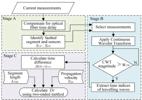
The proposed fault location algorithm consists of three stages as illustrated in Figure 4.

Figure 4: Protection algorithm of fault location scheme.

The first stage (Stage A) of the algorithm identifies the faulted segment. This is implemented by calculating the differential current ∆i(f) for every pair of adjacent sensors

(similarly to equation (1)). When a fault occurs between two sensors, the differential current ∆i(f) calculated from

measurements acquired from those sensors reaches much higher level than the current captured from any other adjacent pair (this was also demonstrated in Figure 3a). As such, by identifying the highest differential current, the faulted segment is identified. At this point the algorithm will produce two outputs: Sup and Sdn for the sensors located upstream downstream to the fault respectively.

Since the faulted segment has been identified in Stage A, post-fault current measurements corresponding to sensors

Sup andSdn are utilised at the next stage (StageB). These measurements are used to calculate the precise time of travelling wave arrival at faulted segment terminals (where the sensors Sup and Sdn are located). The wave detection is implemented by applying Continuous Wavelet Transform (CWT) on the available current measurements. The wavelet transform of a functioni(t)can be expressed as the integral of the product ofi(t)and the daughter waveletΨ∗_a,b(t)given by

W Tψi(t) =

Z ∞

−∞

i(t) √1

αΨ

_t

−b a

| {z }

daughter waveletΨ∗ a,b(t)

dt (2)

The daughter waveletΨ∗

a,b(t)is a scaled and shifted version of the mother waveletΨa,b(t). Scaling is implemented by α which is the binary dilation (also known as scaling factor) and shifted by b which is the binary position (also known as shifting or translation). Finally, StageB will produce two outputs:tSup andtSdn which correspond to the time index of

the initial travelling wave at the faulted segment terminals.

In StageC of the proposed algorithm, the actual fault loca-tionDF of the faulted segment is calculated by adopting the conventional, two-ended fault location approach given by

DF =

Lseg−∆t(Sup−Sdn)·vprop

2 (3)

where∆t(Sup−Sdn)is the time difference of the initial

velocity has been calculated according to the conductor geometry).

4.2. Simulation results

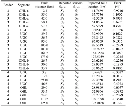
In order to validate the performance of the proposed scheme, pole-to-pole and pole-to-ground faults have been applied on Feeders 3 and 4 (see Figure 1) at various distances at all segments. Since the accuracy of travelling wave-based techniques depend on sampling frequency, for the studies presented in this paper a sampling rate of 135 kHz has been assumed. This frequency corresponds to the resonant frequency of optical sensors and the signal acquisition at this rate can be practically achieved by employing Arrayed Waveguide Grating (AWG) interrogators [13]. The values of fault location estimation error have been reported according to formula (4)

error [%] =DF−ADF

Lf−seg

·100% (4)

whereDF is the calculated fault distance,ADF is the actual fault distance and Lf−seg the total length of the faulted segment.

The results are presented in Tables 5 and 6 for pole-to-pole and pole-to-pole-to-ground faults respectively. The average, minimum and maximum errors observed for pole-to-pole faults correspond to0.3644 %,0.0012 % and1.4625 % re-spectively. For pole-to-ground faults these errors correspond to 0.3955 %, 0.0390 % and 1.3214 % respectively. It can be also seen that the faulted segment has been identified correctly in100 %of the cases for both types of faults (see ‘Reported sensors’ column in Tables 5 and 6).

The impact of noise in measurements, mother wavelet, scal-ing factorαand network components on the accuracy of the proposed fault location scheme, are exhaustively analysed and reported in [5].

TABLE 5: Segment identification and fault location results for pole-to-pole faults.

Feeder Segment _{distance [km]}Fault Reported sensors_S Reported fault Error

U P SDN location [km] [%]

3 OHL-a 12.4 S1 S2 11.7669 -0.9740

3 OHL-a 35.0 S1 S2 35.7736 1.1902

3 OHL-a 42.0 S1 S2 42.3209 0.4937

3 OHL-a 50.1 S2 S3 51.0506 1.4625

3 OHL-a 57.3 S2 S3 57.5979 0.4583

3 UGC 10.0 S2 S3 9.6516 -0.1936

3 UGC 39.7 S2 S3 39.9929 0.1627

3 UGC 56.7 S2 S3 56.8493 0.0829

3 UGC 95.0 S2 S3 95.0569 0.0316

3 UGC 100.0 S2 S3 99.5519 -0.2489

3 UGC 103.0 S2 S3 102.9232 -0.0427

3 UGC 161.2 S2 S3 161.3584 0.0880

3 UGC 173.0 S3 S4 172.5959 -0.2245

3 OHL-b 26.7 S3 S4 26.6210 -0.2256

3 OHL-b 30.0 S3 S4 29.9337 -0.1893

3 OHL-b 33.7 S3 S4 33.8682 0.4806

4 UGC 3.8 S1 S2 3.6487 -0.3027

4 UGC 13.2 S1 S2 13.2006 0.0012

4 UGC 29.10 S1 S2 29.4950 0.7900

4 UGC 46.6 S1 S2 46.3513 -0.4973

4 OHL 29.0 S2 S3 28.9899 -0.0077

4 OHL 53.5 S2 S3 52.9966 -0.3872

4 OHL 74.0 S2 S3 73.7297 -0.2079

4 OHL 110.2 S2 S3 109.7398 -0.3540

4 OHL 125.0 S2 S3 125.0168 0.0129

TABLE 6: Segment identification and fault location results for pole-to-ground faults (Rf = 500 Ω).

Feeder Segment _{distance [km]}Fault Reported sensors_S Reported fault Error

U P SDN location [km] [%]

3 OHL-a 8.1 S1 S2 8.4933 0.6051

3 OHL-a 23.8 S1 S2 24.5979 1.2276

3 OHL-a 35.6 S1 S2 35.7736 0.2671

3 OHL-a 46.5 S1 S2 46.6858 0.2858

3 OHL-a 55.5 S1 S2 55.4155 -0.1300

3 UGC 8.8 S2 S3 8.5278 -0.1512

3 UGC 12 S2 S3 11.8991 -0.0561

3 UGC 33 S2 S3 33.2504 0.1391

3 UGC 56.4 S2 S3 56.2874 -0.0626

3 UGC 100 S2 S3 100.1138 0.0632

3 UGC 144.3 S2 S3 144.5021 0.1123

3 UGC 156 S2 S3 155.7396 -0.1447

3 UGC 165.7 S2 S3 165.8534 0.0852

3 UGC 177.5 S2 S3 177.6528 0.0849

3 OHL-b 15.2 S3 S4 15.3176 0.3359

3 OHL-b 34 S3 S4 33.8682 -0.3765

4 UGC 5.1 S1 S2 5.3343 0.4686

4 UGC 28 S1 S2 28.3713 0.7425

4 UGC 42 S1 S2 42.4182 0.8364

4 UGC 48.5 S1 S2 49.1607 1.3214

4 OHL 4 S2 S3 2.8008 -0.9225

4 OHL 66 S2 S3 66.0912 0.0702

4 OHL 83.5 S2 S3 83.5506 0.0390

4 OHL 99 S2 S3 98.8276 -0.1326

4 OHL 115.7 S2 S3 116.2871 0.4516

5. Hardware Validation of Optical Sensing

Technology

5.1. Experimental Setup

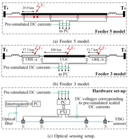
In order to prove the principle of the new protection and fault location scheme an experimental set-up has been arranged as shown in Figure 6 (the actual laboratory experiment is shown in Figure 5). For the realisation of such an experimental set-up the following key components were required:

• Four Fibre Bragg Grating optical sensors. • Four transient voltage suppression diodes. • Optical fibre.

• SmartScan interrogator.

• PXIe-8106 controller (National Instruments).

• PXIe-6259 data acquisition card (National

Instru-ments).

• Pre-simulated DC fault currents.

• PC.

Figure 5: Laboratory experimental arrangement.

For the practical implementation of the proposed schemes, pre-simulated fault currents at corresponding four sensing locations have been generated and stored locally to a PC. For the proposed single-ended differential protection scheme, the model of Feeder5has been utilised with one fault placed at

(a) Feeder 5 model.

(b) Feeder 3 model.

(c) Optical sensing setup.

Figure 6: Laboratory arrangement diagram.

scheme, the model of Feeder3has been utilised (see Figure 6b). The pre-simulated fault currents were used to generate replica voltage traces using the data acquisition card. Such voltage waveforms were physically injected to optical sensors and the corresponding data were captured at 5 kHz from the optical interrogator. The sampled data were then stored on a PC for post-processing. Further technical details with regards to the design, operation and installation of optical sensors can be found in [4], [5].

5.2. Experimental results

The measured response of the optical sensors and the pro-tection system to fault at Feeder 5 is illustrated in Figure 7. The recorded DC voltages were used to calculate the differential voltage∆v(corresponding to differential current

∆i(f)described in equation (1)) which is depicted in Figure

7a. It is evident that the differential voltage between sensors

S1 andS2 reaches high values which can be easily detected

by a voltage threshold. The corresponding rate of change of voltagedVdc/dtof the measurements captured from sensors

S1 and S2 stay high within a 0.2 ms time window. The

entire response of the system is of great resemblance to simulation-based results and hence the protection scheme can be considered practically feasible.

The experimental results related to the proposed fault loca-tion scheme (i.e. experimental arrangement shown in Figure 6b) are summarised in Table 7, where they are also com-pared with the simulation-based results. Due to the reduced sampling rate (i.e. 5 kHz), the resulting accuracy of the experimentally-calculated fault location is notably lower. The sampling frequency has a significant impact on the CWT and the extraction of time difference∆t(Sup−Sdn) which is

utilised in equation (3) for the calculation of fault distance. This can be further justified from the values of time differ-ence ∆t(Sup−Sdn) exacted for each fault case, as shown in

0 5 10 15

v [V]

S 1-S2 S

2-S3 S

3-S4

(a) Differential voltage∆v.

0 0.05 0.1 0.15 0.2 0.25 0.3 0.35 0.4 0.45 0.5

Time [s] -1

-0.5 0 0.5 1 1.5

dV

dc

/dt [kV/s]

S 1 S

2

(b) Rate of change of DC voltage∆v.

Figure 7: Optical and protection system response for pre-simulated fault at Feeder5.

Table 7. With regards to faulted segment, the reported sensors

SupandSdndemonstrate that it has been identified correctly at all cases. It should be noted that the resulting diminished accuracy is due to the reduced sampling rate, determined by the available interrogation system. However, the assumed sampling frequency of 135 kHz is practically achievable with other, commercially available equipment.

TABLE 7: Comparison of experimental and simulations re-sults.

Faults F1 F2 F3

Error [%]

Sim. 0.4583 -0.2489 0.4806 Exp. -1.3254 -1.3415 1.0652

|∆t(SU P−SDN)|

[µs]

Sim. 0.17037 0.12592 0.11110 Exp. 0.16249 0.10000 0.11250 Reported sensors

SU P−SDN

Sim. S1, S2 S2, S3 S3, S4 Exp. S1, S2 S2, S3 S3, S4

5.3. Discussion

It has been demonstrated within this paper that optical sens-ing technology can further enhance the overall performance of protection and fault location applications. This has been demonstrated for HVDC applications, however such technol-ogy has been previously utilised in [6]–[10] for protection and control applications in AC systems. The protection, control and fault location schemes have been realised by the employment of optical current and voltage sensors. Such sensors have been designed and manufactured based on magneto-optical constructions based on fibre coils, extrinsic magnetostrictive materials bonded to fibre strain sensors.

fundamental difference of these two applications is that the protection needs to be run in real-time while for distance to fault estimation off-line computations can be used. There-fore, lower sampling rate (i.e. 5 kHz) is adequate to permit computational efficiency and high speed operation of the protection module. However, for fault location applications higher sampling rates have to be used in order to guarantee sufficient fault location accuracy. Since the two proposed schemes utilise the same sensing architecture, there is no reason why they could not coexist sharing the same fun-damental sensing and interrogation hardware, and forming an integrated protection and fault location system. So long as the fault generated waveforms are captured at adequate sampling rate (i.e. in excess of 100 kHz) both protective and fault locating functions could be performed independently in their respective operating time frames. This would satisfy both, the need for high speed of protection operation and high accuracy of fault location. For example, a real-time calculation with operating frame rate in the range of 5 kHz (using down-sampled data) would be adequate for protection, while for fault location a non-real-time post fault calculation could be performed using the stored data acquired at much higher frequency. A circular memory buffer of approximately 100 ms should provide sufficient amount of data to achieve accurate fault position estimation.

For application in electrical power systems, the key technical and economical merits of the utilised distributed sensing technology (compared to other conventional and purely elec-trical), arise from the fact that the sensors are completely passive and require no power supply at the sensing location. Moreover, there is no need for additional signal processing and communication equipment (i.e. micro-controllers, GPS, etc.) at the location of the sensors (i.e. sensors are interro-gated from a single acquisition point, where measurements can be also time-stamped). These technical merits have the potential to enable reduction in the hardware and infrastruc-ture needs (i.e. communications, low voltage power supplies, decoders/encoders, etc.) required for wide-area monitoring applications. It should be also highlighted that over the last decade the cost of optical sensors has been decreased adequately, leading to practical realisation of cheap and high performance transducers. Overall, due to the extensibility and centralised nature of the sensing technology, the capability of distributed sensing is undoubtedly technically beneficial, while in the long-term, it can ultimately lead to reduction of operational and capital expenditure. Since measurements have been made available [14] in standardised sampled value formats (IEC 61850-9-2), it can be considered a ready-to-use technology for substation automation, and for protection and control of electrical networks (from microgrids to large transmission lines).

6. Conclusions

In this paper, a new single-ended differential protection scheme and a fault location scheme for hybrid feeders has been presented. Such schemes were designed for HV-MTDC networks and are based upon the principle of distributed optical sensing. The proposed protection scheme has been found to be highly sensitive, discriminative and fast both for pole-to-pole and pole-to-ground faults. With regards to fault location in hybrid feeders, the proposed travelling wave-based algorithm, has been found to be capable of identifying

the faulted segment, while maintaining high accuracy of the fault location estimation across a wide range of fault sce-narios. The overall performance of both schemes have been assessed through transient simulation and further validated using small-scale hardware prototypes and hardware-in-the-loop testing. The potential technical and economical benefits of distributed sensing technology have been also discussed within the paper.

7. Acknowledgements

This work was supported by Royal Society of Edinburgh (J M Lessells Travel Scholarship), Synaptec Ltd | Glasgow -UK, the Innovate UK (TSB Project Number 102594) and the European Metrology Research Programme (EMRP) -ENG61. The EMRP is jointly funded by the EMRP partici-pating countries within EURAMET and the European Union.

References

[1] D. Tzelepis, A. O. Rousis, A. Dysko, C. Booth, and G. Strbac, “A new fault-ride-through strategy for MTDC networks incorporating wind farms and modular multi-level converters,”Electrical Power and Energy Systems, vol. 92, pp. 104–113, November 2017.

[2] D. V. Hertem and M. Ghandhari, “Multi-terminal VSC-HVDC for the european supergrid: Obstacles,” Renewable and Sustainable Energy Reviews, vol. 14, no. 9, pp. 3156 – 3163, 2010.

[3] D. Tzelepis, S. Ademi, D. Vozikis, A. Dysko, S. Subramanian, and H. Ha, “Impact of VSC converter topology on fault characteristics in HVDC transmission systems,” inIET 8th International Conference on Power Electronics Machines and Drives, March 2016.

[4] D. Tzelepis, A. Dyko, G. Fusiek, J. Nelson, P. Niewczas, D. Vozikis, P. Orr, N. Gordon, and C. D. Booth, “Single-ended differential pro-tection in MTDC networks using optical sensors,”IEEE Transactions on Power Delivery, vol. 32, no. 3, pp. 1605–1615, June 2017.

[5] D. Tzelepis, G. Fusiek, A. Dyko, P. Niewczas, C. Booth, and X. Dong, “Novel fault location in MTDC grids with non-homogeneous trans-mission lines utilizing distributed current sensing technology,”IEEE Transactions on Smart Grid, 2017,‘Early Access Articles’.

[6] P. Orr, G. Fusiek, C. D. Booth, P. Niewczas, A. Dyko, F. Kawano, P. Beaumont, and T. Nishida, “Flexible protection architectures using distributed optical sensors,” in Developments in Power Systems Pro-tection, 11th International Conference on, April 2012, pp. 1–6.

[7] P. Orr, G. Fusiek, P. Niewczas, C. D. Booth, A. Dyko, F. Kawano, T. Nishida, and P. Beaumont, “Distributed photonic instrumentation for power system protection and control,” IEEE Transactions on Instrumentation and Measurement, vol. 64, no. 1, pp. 19–26, Jan 2015.

[8] P. Orr, C. Booth, G. Fusiek, P. Niewczas, A. Dysko, F. Kawano, and P. Beaumont, “Distributed photonic instrumentation for smart grids,” inApplied Measurements for Power Systems,IEEE International Work-shop on, Sept 2013, pp. 63–67.

[9] G. Fusiek, P. Orr, and P. Niewczas, “Temperature-independent high-speed distributed voltage measurement using intensiometric FBG in-terrogation,” inIEEE International Instrumentation and Measurement Technology Conference, May 2015, pp. 1430–1433.

[10] P. Orr, G. Fusiek, P. Niewczas, A. Dyko, C. Booth, F. Kawano, and G. Baber, “Distributed optical distance protection using FBG-based voltage and current transducers,”2011 IEEE Power and Energy Society General Meeting, pp. 1–5, July 2011.

[11] P. Niewczas and J. R. McDonald, “Advanced optical sensors for power and energy systems applications,”IEEE Instrumentation Measurement Magazine, vol. 10, no. 1, pp. 18–28, Feb 2007.

[12] M. Callavik, A. Blomberg, J. Hafner, and B. Jacobson, “The hybrid HVDC breaker,” inABB Grid Systems, November 2012.

[13] G. Fusiek, P. Niewczas, and J. McDonald, “Feasibility study of the application of optical voltage and current sensors and an arrayed waveguide grating for aero-electrical systems,”Sensors and Actuators A: Physical, vol. 147, no. 1, pp. 177 – 182, 2008.