Numerical and Experimental Analysis of Transient Flow in Roots Blower

(1)

City, University of London Institutional Repository

Citation:

Sun, S. H., Kovacevic, A., Bruecker, C., Leto, A., Singh, G. and Ghavami, M. (2018). Numerical and Experimental Analysis of Transient Flow in Roots Blower. IOP Conference Series: Materials Science and Engineering, 425, 012024.. doi: 10.1088/1757-899X/425/1/012024

This is the published version of the paper.

This version of the publication may differ from the final published

version.

Permanent repository link:

http://openaccess.city.ac.uk/21360/

Link to published version:

http://dx.doi.org/10.1088/1757-899X/425/1/012024

Copyright and reuse: City Research Online aims to make research

outputs of City, University of London available to a wider audience.

Copyright and Moral Rights remain with the author(s) and/or copyright

holders. URLs from City Research Online may be freely distributed and

linked to.

City Research Online: http://openaccess.city.ac.uk/ [email protected]

(2)

IOP Conference Series: Materials Science and Engineering

PAPER • OPEN ACCESS

Numerical and Experimental Analysis of Transient Flow in Roots Blower

To cite this article: S H Sun et al 2018 IOP Conf. Ser.: Mater. Sci. Eng. 425 012024

(3)

1

Content from this work may be used under the terms of theCreative Commons Attribution 3.0 licence. Any further distribution of this work must maintain attribution to the author(s) and the title of the work, journal citation and DOI.

Published under licence by IOP Publishing Ltd

1234567890_‘’“”

International Conference on Screw Machines 2018 IOP Publishing

IOP Conf. Series: Materials Science and Engineering 425_{(2018) 012024 doi:10.1088/1757-899X/425/1/012024}

Numerical and Experimental Analysis of Transient Flow in

Roots Blower

S H Sun1,2*, A Kovacevic2*, C Bruecker3, A Leto2,4, G Singh2 and M Ghavami2 1_{Xi’an University of Technology, No.5, South Jinhua Road, 710048, CHINA.}

2

Centre for Compressor Technology, City University London, EC1V0HB, UK. 3

Sir Richard Oliver Chair in Aeronautical Engineering, City University London, EC1V0HB, UK.

4_{Faculty of Mechanical Engineering, Džemal Bijedić University of Mostar, University}

Campus, 88104, Bosnia & Herzegovina. * Corresponding Author.

Email: [email protected], [email protected].

Abstract. The performance of rotary positive displacement machines highly depends on the

operational clearances. It is widely believed that computational fluid dynamics (CFD) can help understanding internal leakage flows. Developments of grid generating tools for analysis of leakage flows by CFD in rotary positive displacement machines have not yet been fully validated. Roots blower is a good representative of positive displacement machines and as such is convenient for optical access in order to analyse internal flows. The experimental investigation of flow in optical roots blower by phase-locked PIV (Particle Image Velocimetry) performed in the Centre for Compressor Technology at City, University of London provided the velocity field suitable for validation of the simulation model. This paper shows the results of the three-dimensional CFD transient simulation model of a Roots blower with the dynamic numerical grids generated by SCORG and flow solution solved in ANSYS CFX flow solver to obtain internal flow patterns. The velocity fields obtained by simulation agree qualitatively with the experimental results and show the correct main flow features in the working chamber. There are some differences in the velocity magnitude and vortex distribution. The flow field in roots blower is highly turbulent and three-dimensional. The axial clearances should be included, and the axial grids should be refined in the simulation method. The paper outlines some directions for future simulation and experimental work. The work described in this paper is a part of the large project set to evaluate characteristics of the internal flow in rotary positive displacement machines and to characterize leakage flows.

1. Introduction

(4)

1234567890_‘’“”

performance. The challenge is to maintain the size of the gaps due to deformations of the machine elements which could be caused by thermal of physical loads.

Many researchers have studied leakage flows through clearance gaps in rotary positive displacement machines both experimentally and numerically. Numerical methods are mostly based either on chamber modelling [1], or computational fluid dynamics (CFD) model [2, 3]. In chamber models, it is usually assumed that the momentum change in the main domain is negligible due to the internal energy being dominant while the velocity of the leaking fluid is obtained based on the assumption of the isentropic flow through the nozzle. A CFD model allows more accurate calculation of velocities both in the main domain and in the leakage paths by numerically solving governing conservation equations such as mass, energy and momentum. This is of course subject to availability of an accurate numerical mesh which can capture both, the main flow domain and clearances. The latest developments in grid generation for screw machines described in detail in Rane et al. [4, 5] have led to the mesh which can be used in all flow calculations and for most rotary positive displacement machines. This grid generation methods allows use of any commercially available CFD solvers. The size of the mesh, the speed of its generation as well as the speed of calculation by commercial solvers is suitable for industrial application. However, it is yet not fully validated if it sufficiently accurately captures flow in clearances.

Numerical procedures for calculation of performance using either chamber models or 3D CFD are usually validated by measurements of the integral parameters such as the total mass flow rate and power as shown in recent studies by Kovacevic and Rane [6]. These indicate that the clearance flow is mostly well captured. However, unless the local velocities are measured, the leakage models cannot be fully validated. In addition, even the velocity distribution in the main flow of a rotary positive displacement machine has not been studied in detail experimentally. Therefore, for the full validation of numerical calculations it is required to obtain accurate measurements of the flow field both in the main working domain and in the clearance gaps of a rotary positive displacement machine.

Attempts were made in the past to evaluate local flows in screw compressors using optical methods. Firstly, Sachs [7] studied the gas flows in the tip gap of a static flat rotor screw compressor experimentally. The Toppler schlieren method was applied to obtain the swirls image in the leakage gap. The influence of pressure ratio, gap shape, gap height and moving boundary on the schlieren image were investigated. And the mass flow rate and velocity near the gap were compared. The boundary layer separation, swirls and Mach wave were also shown. The LDV method was recommended to obtain quantitative results in the gap without interference with the leakage flow. The Laser Doppler Velocimetry (LDV) measurements in the working chamber close to the discharge and in the discharge chamber of an oil free compressor were reported by Gueratto et al. [8] while the measurement of the flow in the suction chamber of an oil free compressor with water injection were reported by Kovacevic et al. [9]. However, neither of these managed to give quantitative velocity values within the working domain of the compressor and in the clearances. Screw machines with helical rotors are difficult to modify in order to provide optical access for the assessment of flow. The alternative is a roots blower which has straight lobes and similar characteristics of the flow as screw machines.

Roots blowers usually have two straight rotors with an involute profile and two or more lobes in each. The rotors rotate in the opposite directions within the casing and form a working chamber between the rotors and casing. Roots blowers do not have internal compression as the volume of the chamber remains constant while rotating. The increase of the pressure is external to the rotors due to the backflow from the high-pressure side. Recently, Liu et al. [10, 11] and Sun et al. [12, 13] established the CFD simulation model of the roots blower and validated it by measurements of mass flow rate and pressure distribution. In addition, the leakage flow in a two-lobe roots blower was predicted using a stationary mesh in CFD and the results were compared with the experimental leakage mass flow rate [14]. The development of experimental techniques to determine velocities using optical methods have been reported recently by Sun et al. [15].

(5)

phase-3

1234567890_‘’“”

locked PIV (Particle Image Velocimetry) performed in the Centre for Compressor Technology at City, University of London [15] was used to validate the simulation model. The simulation and experimental velocity fields are analysed and compared. The work described in this paper is a part of the large project set to evaluate characteristics of the internal flow in rotary positive displacement machines and to characterize leakage flows with the objective to lead to further improvements in 3D CFD analysis of leakage flows in rotary positive displacement machines and ultimately lead to the improvement in the performance of rotary positive displacement machines.

2. Simulation model

2.1. Physical Model

[image:5.595.85.511.341.494.2]

This paper studies a roots blower with two-lobed rotors mounted on parallel shafts that rotate in opposite directions to transfer air as working fluid. The physical model is shown in Figure 1. The suction and discharge pipes connect to the inlet and outlet domains respectively. The air passes into the roots blower through the inlet and fills into the suction chamber formed by the casing and rotor. The female rotor rotates clockwise, and the reference crank angle when the female rotor is vertical is defined as 0°. Three types of gaps are recognised in the roots blower, namely the tip gap, the interlobe gap and the axial gap between the side of the lobes and the casing. The main dimensions are shown in Table 1.

Figure 1. Physical model of roots blower at crank angle 10 ° and 100 °. Table 1. The main parameters of the roots blower.

Items Specification Items Specification

Diameter of the rotor/mm 101.3 Tip gap/mm 0.1

Axis distance/mm 63.12 Interlobe gap/mm 0.17

Rotor length/mm 50.5 Axial gap/mm 0.15

Displacement volume/ l/rev 0.4618 Width of tip step/mm 6.4

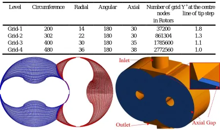
2.2. Grid generation

[image:5.595.67.531.535.605.2]

(6)

1234567890_‘’“”

(1)

[image:6.595.76.523.229.493.2]

where Z is the number of lobes, and n is the rotation speed (rpm). Inversely, the angular divisions can be calculated out when the simulation time step is given. As shown in the right of Figure 2, the stationary grids consist of inlet grids, outlet girds and axial-gap grids which have six layers of grids in each axial gap. The lengths of suction pipe and discharge pipe are three and nine times of the pipe diameter. Hexahedral grids with 889405 nodes for the stationary grids were generated in ANSYS-Mesh and used in all cases. The rotor grids and the stationary grids are combined and connected with interfaces.

Table 2. Grid levels and number divisions.

Level Circumference Radial Angular Axial Number of grid

nodes in Rotors

Y+ at the centre line of tip step

Grid-1 200 14 180 30 37200 1.8

Grid-2 302 22 180 30 861304 1.3

Grid-3 400 30 180 35 1785600 1.1

Grid-4 480 36 180 38 2772560 1.0

Figure 2. The rotor grids and the whole grids.

2.3. Simulation model boundary condition setting

The Ansys -CFX solver was used for the calculation of the roots blower. The working fluid was air as ideal gas. The high-resolution scheme was used for the advection term while the second order backward Euler scheme was used for the transient term. The SST (Shear Stress Turbulence) turbulence model was adopted in the calculation. The Y+ at the centre line of the lobe tip step was checked and was lower than 2 in all cases, as shown in Table 2. The time step was 3.592E-4 as determined by equation (1) for the rotor speed of 464rpm. The number of iterations was 10 for every time step. The static pressure was used respectively for the inlet and outlet opening boundaries. The pressure at the inlet and outlet was given as measured ones during the experiment.

3. Experimental setup

(7)

5

1234567890_‘’“”

sustain only limited temperatures which was achieved by low speeds and pressures. The test at the practical operating conditions will follow in future.

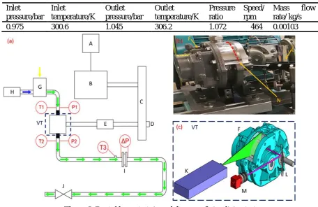
Table 3. Operating conditions for the roots blower tests.

Inlet

pressure/bar Inlet

temperature/K

Outlet pressure/bar

Outlet

temperature/K

Pressure ratio

Speed/ rpm

Mass flow

rate/ kg/s

[image:7.595.67.524.140.436.2]

0.975 300.6 1.045 306.2 1.072 464 0.00103

Figure 3. Roots blower test rig and diagram of visualizing test.

A - inverter, B – electromotor, C- pulleys, D – shaft encoder, E- torque meter, F – roots blower, G – smoke tank, H – smoke machine, I – orifice plate, J – valve, K – double pulse laser, L – surface mirror, M – double shutter camera, N – Position of Laser plane, T1 – suction temperature transducer, P1 – suction pressure transducer, T2 –

discharge temperature transducer, P2 – discharge pressure transducer, T3 – upstream temperature transducer, ΔP – differential pressure across an orifice plate

(8)

1234567890_‘’“”

intervals of 30 °. The crank angles of shooting position are 10, 40, 70, 100, 130 and 160° respectively. Figure 1 shows the rotor positions at the crank angle of 10 and 100 °. The PIV results were processed using Dantec Dynamic studio by the adaptive PIV approach.

4. Results and discussion

4.1 Grid independence

Four cases with different grid density have been solved using Ansys CFX solver at the operation condition in Table 3. The cycle average mass balance between the rotor suction and discharge was achieved within 3% in all cases. Figure 4 shows the variation of the mass flowrate of the roots blower at various rotor grid refinements. The mass flow rate difference between the third level of the refinement and the fourth one is 4.0 %, which is far lower than the difference between the first level and second level. Therefore, the third level grids are regards as the enough fine grids. Because the interface between the two rotors in rotor to casing grids will influence the mass flow rate of the rotary machine [6], the casing to rotor grids which have the same divisions and nodes number with those of rotor to casing grids of Grid-3 were generated to be used in the simulation model whose results are selected for further analysis and compared with the experimental results.

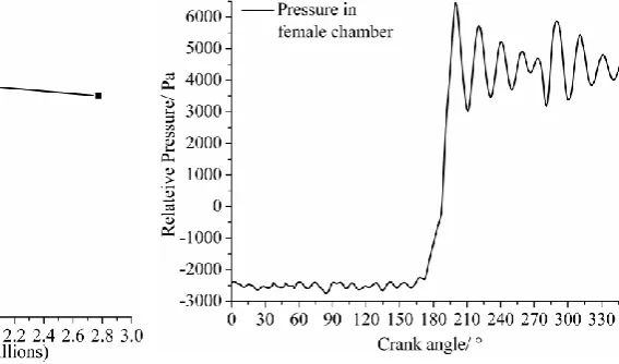
4.2 Pressure variation and Mass flow rate

Figure 5 shows the static relative pressure variation in the working chamber formed by the female rotor and the casing. The reference pressure to compute this variation is 1bar. It is suction process when the crank angle moves from 0 to 180 °, and the discharge process corresponds to the 180 to 360 °. The pressure begins to increase at 170 ° and reach to maximum value at 200 °. It is mainly because of the tip step on the lobe which makes the suction chamber to close earlier and opens later, and finally extends the compression process and reduces the leakage flow during the process. There are two similar periodic pressure fluctuations during this process, and the second one begins at 270°. During every pressure fluctuation process, the pressure fluctuates sharply at the beginning and damps at the end, which has the inverse relation with the outlet mass flow rate shown in Figure 6. When the mass flow rate increases, the pressure decreases. If the crank angle reaches 270 °, the working chamber formed by the male rotor and the casing connects with the discharge chamber, so the outlet mass flow rate falls as shown in Figure 6, and the pressure in the female chamber increases, which leads to the second periodic pressure fluctuation.

Figure 4. Grid independence analysis of a Roots blower rotor computational domain.

Figure 5. Pressure variation in working chamber.

[image:8.595.232.516.503.670.2]

(9)

7

1234567890_‘’“”

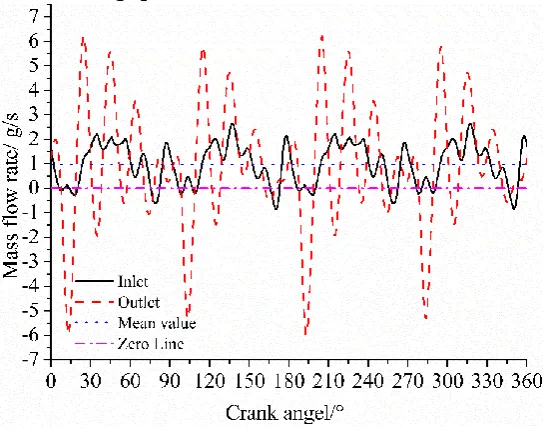
under low pressure difference. In Figure 6, the total cycle has four repeated suction and discharge process. Because this roots blower has two same rotors which have two symmetric lobes respectively, the suction or discharge chamber formed by male rotor is symmetrical with that formed by the female rotor and has a period of 180 °. Hence, four periodic suction and discharge process appear, which also results in the two cycles of discharge pressure as shown in Figure 5. When the female lobe is at its vertical position, the crank angle is 0 °, as shown in Figure 1. Both inlet and outlet mass flow rate fluctuate with the crank angle. The outlet mass flow rate has higher pulsations than the corresponding inlet value. The reverse flow often happens at the outlet surface if the mass flow rate is negative. The maximum backflow rate of 5.9 g/s occurs at 15° and195° when the closed working chamber formed with female rotor connects with the discharge chamber. At that moment, the high pressure working fluid flows back into the working chamber, and the pressure in the working chamber increases quickly to the discharge pressure.

Figure 6. Inlet and outlet mass flow rate.

4.3 Comparison between the experimental and simulation results

[image:9.595.73.345.257.472.2]

Figure 7 shows the original figures from the standard PIV test at the shooting position of 10 ° and 100 °. The tracked particles can be distinguished easily in both pictures. At the crank angle of 10 °, the windows show the front of the lobe which has just closed the suction. At the crank angle of 100°, the window shows the area behind the lobe connected to the suction chamber. Two shadows caused by the bolts installed in the window (marked as 1 and 2) are visible in the frames, one at the top left of the window and another on the right side of the window which reduce the visible flow field.

[image:9.595.81.515.575.742.2]

(10)

1234567890_‘’“”

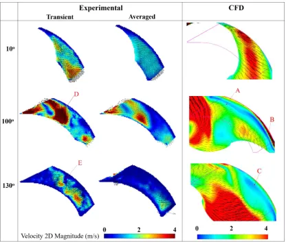
[image:10.595.92.509.357.710.2]

The simulation and experimental results are compared in Figure 8. The velocity fields at three positions are displayed and compared. The colour bars of experimental and CFD results show the velocity magnitude in the plane of the laser sheet. The experimental results include the transient velocity flow field and average values obtained by averaging the transient velocity vectors from all 120 measured cycles. The simulation results are obtained from the results of next rotation cycle after the simulation was converged. The velocity vectors were calculated in the laser sheet plane. The black frame superimposed on the CFD results represents the border of visible area of the PIV pictures, so that the flow field in the frame can be compared with the measured velocity field. Comparing the simulation velocity field with the averaged PIV results, the fluid mainly flows downward at 10°; at 100°, the fluid in the two images flows from the bottom to the top and then is divided into two regions of flow movement. At 130°, most of fluid in the black frame moves towards the casing side. Hence, the simulation velocity fields have the similar flow features with the averaged PIV results. However, there are still obvious difference between the simulation and experimental average results. Firstly, the velocity magnitude of the simulation is larger than the experimental values. Also, the simulation velocity flow fields are more turbulent than the averaged PIV values which do not have the flow pattern in the same area A and C of the corresponding simulation images. In the simulation results of 100 °, the back flow in area B is caused by the tip leakage flow whose velocity decreases along the casing wall. The back flow and the main flow mixes and forms a low-velocity stripe, as shown in area A. The low-velocity area C results from the same reason. The experimental results do not show the same flow pattern, which implies that the simulation tip leakage flow may be overestimated.

Figure 8. Comparison between the PIV results and CFD results at various crank angle positions.

(11)

9

1234567890_‘’“”

in transient flow field are more similar to simulation flow field. But the transient flow field has more turbulence characteristics such as the vortex in areas D and E. Hence, the simulation results show the correct main flow features in the working chamber, but they have differences in the velocity magnitude and vortex distribution.

Usually, it is difficult to compare the transient PIV results with the URANS (Unsteady Reynolds-averaged Navier–Stokes) simulation results because the simulation model calculates the time-average velocity and adopts the Reynolds stress transport equations to impose the influence of turbulence on the time-average velocity. Some researchers use the simulation results of LES (Large Eddy Simulation) to compare with the transient PIV results [16, 17]. There is an indication that the simulation results agreed well with simulation results.

Many researchers compared the RANS or URANS simulation results with the time-average PIV results. Mortensen et al. [18] compared the simulation results of a rotor stator mixer from e, SST k-w and RSM (Reynolds stress model) k-with the time-average PIV results and found that simulation results over-predicted the dissipation rate of the TKE (turbulent kinetic energy) and indicated that the realizable k-e model was better than the other two turbulence models. Zou et al. (2016) used the standard k-e model to simulate the two-phase flow in a pump mixer and compared the simulation results with the PIV results, the deviation velocity error changes from 16.5% to 33%. Ryan et al. [19] adopted the SST-SAS (Scale adaptive simulation) turbulence model in the simulation of a sonolator liquid whistle and compared the simulation results with PIV time-averaged results. The simulation velocity agreed well with the experimental one, but the turbulence parameters matched with the experimental one poorly. Kurec et al. [20] had done simulation with standard k-w, SST k-w and SST-SAS turbulence model in a pressure exchange passage and validated the simulated results with PIV results. The comparison showed that the SST-SAS model can provide best prediction of the three turbulence models, but the simulation results are more turbulent than the PIV time-average results. Both Ryan et al. [19] and Kurec et al. [20] hinted that the CFD results needed to be averaged with different cycles because the PIV time-average results almost removed most of the turbulence features of the transient flow. Therefore, for our simulation, the CFD time-average results of several cycles will be firstly done to check if the simulation results can be improved, and then the SST-SAS model will be used in our simulation. LES simulation will be the last one because it requires a large amount of computational resources.

4.4 Analysis of the main velocity field

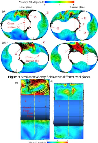
The experimental results can only capture a part of the domain while the simulation model can provide the whole 3D flow fields which can help to investigate the physical nature of the internal flow in a Roots blower. Figure 9 shows the whole simulation flow fields at two different axial planes. The flow fields in the left column are on the laser plane as shown in Figure 3. The crank angles are 10 ° and 100 ° which are same with the first two angles in Figure 8, so the downstream and upstream of the partial velocity fields in Figure 8 can be obtained. The velocity field in the right column are on the central plane which locates at the centre between the two side walls. Figure 10 displays the velocity flow fields in the cross sections along the axial direction. The cross section (a), is located in the mid-point between the centres of two rotors when the crank angle is 10 °; and the cross-section (B) which is also marked in Figure 9 is located at the one third of radius of the female lobe when the crank angle is 100 °. In addition, the axial positions of the central plane and the laser plane are shown in both cross sections of Figure 10. From Figure 9, the velocity direction in area A and C on the laser plane are opposite to that on the central plane. The reason is that the velocity field is three dimensional.

(12)

1234567890_‘’“”

symmetrical axial boundary condition is not clear. The unsteady simulation may contribute to this phenomenon.

Hence, the velocity field in roots blower is highly turbulent three-dimensional flow. The axial leakage clearance should not be neglected, or else the velocity field on the laser plane in Figure 8 will certainly

[image:12.595.127.467.253.746.2]

have big deviations with the PIV test results. Furthermore, the axial grids should be refined to improve the accuracy of simulation results. and the laser plane can move along the axis and measure the flow field at several planes including the central plane to validate the three-dimensional flow field. The situation is the same at the area B in Figure 9 where the fluid flows downward, but the fluid in central plane at the same area flows toward to the lobe. Apparently, there is one source D which results in the upward flow which influence the velocity direction at the area B of central plane. It is also caused by the three-dimensional flow.

Figure 9. Simulation velocity fields at two different axial planes.

(13)

11

1234567890_‘’“”

The tip and interlobe leakages have different influence on the flow field as shown in Figure 9. The tip leakage has important influence on the downstream flow field of laser plane where it causes the low-velocity stripe while it has slight influence on the flow filed of central plane. It is because the main flow velocity on the central plane is bigger than that on the laser plane.

The maximum velocity in tip gap E is about 50m/s while the maximum velocity in the lobe gap F is 80m/s, which means the leakage flow rate through the lobe gap is far higher than that through the tip leakage. The interlobe leakage obviously influences the main flow pattern, as shown in Figure10a. In the laser plane, the interlobe leakage velocities have the same direction as the main flow, so it reinforces and accelerates the main flow such as the flow field G. However, in the central plane, the interlobe leakage flow velocities have the opposite direction with the main flow, so their influences are supressed. The leakage flow velocities reverses and the vortices H and I generate on the central plane.

5. Conclusions

The three-dimensional CFD transient simulation model of a Roots blower was established to obtain the internal flow field. The standard PIV test was conducted on the optical roots blower with transparent windows to validate the simulation model. The outlet mass flow has higher pulsations than the inlet mass flow. The maximum back flow happens when the working chamber connects to the outlet. The simulation velocity fields have similar features to the experimental results and show the correct main flow direction in the working chamber, but they show differences in the velocity magnitude and vortex distribution. Two asymmetric vortices exist on the cross section which leads the downward flow on the central plane and upward flow on the laser plane. The side leakage flow through the axial clearance has an important effect on the formation of the two vortices while the interlobe leakage makes the two vortexes asymmetrical. Therefore, the flow field in roots blower is highly turbulent and three dimensional. The axial clearance should not be neglected, and the axial grids should be refined, in order to ensure the correctness of the simulation model. The interlobe leakage is larger than the tip leakage and affects the flow field significantly. It reinforces the main velocity field of the side flow (laser plane) and suppresses the flow in the central plane.

The future work will be conducted both on the improvement of the simulation model and the PIV test. The SST-SAS model will be used in simulation to improve the accuracy further. And the LES simulation will be considered at last. For the PIV test, the laser plane will be moved within the available domain to validate the prediction of the simulation model. And the microscope lens will be used to investigate the leakage flow. The operation speed and the pressure ratio will increase gradually, according to the quality of test results. The final objective of this research is to improve the 3D CFD analysis of leakage flows and ultimately lead to the improvement in the performance of rotary positive displacement machines.

References

[1] Stošić N, Smith I K and Kovačević A 2005 Screw Compressors: Mathematical Modelling and Performance Calculation (Berlin: Springer-Verlag)

[2] Kovacevic A 2005 Boundary adaptation in grid generation for CFD analysis of screw compressors International Journal for Numerical Methods in Engineering64 401-26

[3] Kovačević A, Stošić N and Smith I K 2007 Screw compressors - Three-dimensional computational fluid dynamics and solid fluid interaction (Berlin: Springer-Verlag)

[4] Rane S 2015 Grid Generation and CFD analysis of variable Geometry Screw Machines. (London: City, University of London)

[5] Rane S and Kovacevic A 2017 Algebraic generation of single domain computational grid for twin screw machines. Part I. Implementation Advances in Engineering Software107 38-50 [6] Kovacevic A and Rane S 2017 Algebraic generation of single domain computational grid for

twin screw machines Part II – Validation Advances in Engineering Software109 31-43

(14)

1234567890_‘’“”

[8] Guerrato D, Nouri J M, Stosic N, Constantine A and Smith I K 2007 Flow measurements in the discharge port of a screw compressor Proceedings of the Institution of Mechanical Engineers, Part E: Journal of Process Mechanical Engineering222 201-10

[9] Kovacevic A, Arjeneh M, Rane S, Stosic N and Gavaises M 2014 Flow Visualization at Suction of a Twin Screw Compressor. In: International Screw Compressor Conference 2014,

(Dortmund: VDI Verlag Gmbh)

[10] Liu X M, Lu J, Gao R H and Xi G 2013 Numerical Investigation of the Aerodynamic Performance Affected by Spiral Inlet and Outlet in a Positive Displacement Blower Chinese Journal of Mechanical Engineering26 957-66

[11] Liu X M and Lu J 2014 Unsteady Flow Simulations in a Three-lobe Positive Displacement Blower Chinese Journal of Mechanical Engineering27 575-83

[12] Sun S K, Zhao B, Jia X H and Peng X Y 2017 Three-dimensional numerical simulation and experimental validation of flows in working chambers and inlet/outlet pockets of Roots pump

Vacuum137 195-204

[13] Sun S K, Jia X H, Xing L F and Peng X Y 2018 Numerical study and experimental validation of a Roots blower with backflow design Engineering Applications of Computational Fluid Mechanics12 282-92

[14] Ashish M. Joshi, David I. Blekhman, James D. Felske, John A. Lordi and C.Mollendorf J 2006 Clearance Analysis and Leakage Flow CFD Model of a Two-LobeMulti-Recompression Heater

International Journal of Rotating Machinery2006 1-10

[15] Sun S H, Kovacevic A, Bruecker C, Leto A, Ghavami G, Rane S and Singh G 2018 Experimental Investigation of the Transient Flow in Roots Blower. In: 24th International Compressor Engineering Conference, (Chicago: Purdue university)

[16] Ji B, Luo X W, Arndt R E A, Peng X and Wu Y 2015 Large Eddy Simulation and theoretical investigations of the transient cavitating vortical flow structure around a NACA66 hydrofoil

International Journal of Multiphase Flow68 121-34

[17] Liu M, Gao Z, Yu Y, Li Z, Han J, Cai Z and Huang X 2018 PIV experiment and large eddy simulation of turbulence characteristics in a confined impinging jet reactor Chinese Journal of Chemical Engineering

[18] Mortensen H H, Arlov D, Innings F and Håkansson A 2018 A validation of commonly used CFD methods applied to rotor stator mixers using PIV measurements of fluid velocity and turbulence Chemical Engineering Science177 340-53

[19] Ryan D J, Simmons M J H and Baker M R 2017 Determination of the flow field inside a Sonolator liquid whistle using PIV and CFD Chemical Engineering Science163 123-36

[20] Kurec K, Piechna J and Gumowski K 2017 Investigations on unsteady flow within a stationary passage of a pressure wave exchanger, by means of PIV measurements and CFD calculations

Appl. Therm. Eng.112 610-20

Acknowledgement

The author would like to thank Howden Compressors for allowing authors to use and modify one of the Howden Roots Blowers in this experiment.

The authors gratefully acknowledge financial support from China Scholarship Council (CSC) to allow the researcher from China to perform this work at City, University of London.