Influence of Molecule–Surface and
Molecule-Molecule Interactions on
Two-Dimensional Patterns formed by
Functionalised Aromatic Molecules
Sara Fortuna
∗,†,‡and Karen Johnston
∗,¶†Department of Chemical and Pharmaceutical Sciences, University of Trieste, Via L.
Giorgieri 1, 34127 Trieste, Italy
‡http://www.sarafortuna.eu
¶Department of Chemical and Process Engineering, University of Strathclyde, James Weir
Building, 75 Montrose Street, Glasgow, G1 1XJ, United Kingdom
Abstract
Molecules self-assemble on surfaces forming a variety of patterns that depend on
the relative strength between the intermolecular and molecule–surface interactions. In
this study, the effect of the physisorption/chemisorption interplay on self-assembly is
investigated using Monte Carlo simulations. The molecules are modelled as hexagonal
tiles capable of assuming two distinct adsorption states, with different diffusion
prop-erties, on a hexagonal lattice. The self-assembled structures that emerge by tuning
the molecule–surface and molecule–molecule interactions are systematically mapped
out to develop understanding of their phase behaviour. The resulting phase diagrams
will guide the engineering of novel molecules to obtain desired collective structural
properties for development of innovative two-dimensional devices.
1. Introduction
Controlling the self-organisation of molecular adlayers is key for the development of novel
two-dimensional devices, such as graphene nanostructure spintronics1 or conjugated
aro-matic polymer anodes for ion batteries.2 While the nature and strength of molecule–surface
interactions control the interfacial and electronic properties of adsorbed molecules, the
mono-layer patterns formed are controlled by the interplay between molecule–surface and molecule–
molecule interactions.3 Therefore, in order to control the monolayer structure, one can adjust
the interactions by changing the chemical properties of the molecular adlayer.
Molecular functionalisation,4 such as the introduction of groups capable of
hydrogen-bonding5 or bulky groups,6 is one way to adjust the molecular interactions and is well
documented to affect the observed monolayer patterns.7–9 Halogenation of molecules can
heavily modify these patterns, especially for aromatic molecules. For instance pentacene
is known to form two different ordered phases on Au(111) but its fluorination leads to
the formation of only one single phase, in the form of ordered arrays.10 Further examples
non-standard molecule–surface coupling that is stronger than typical physisorption but weaker
than chemisorption leading to a variety of self-assembled patterns and surface
reconstruc-tions.11,12 In this case the assemblies can be further controlled by fluorination, as observed
for copper phtalocyanine patterning on Cu(100) and Cu(111).13 The effect of fluorination
on monolayer structure is also observed in benzene on metal surfaces.14,15
In all cases, molecular functionalisation controls the interaction parameters that drives
the system towards a particular monolayer structure3 and there are striking examples where
functionalised molecules exist in two or more distinct adsorption states. Kohn-Sham density
functional theory calculations have found that that on platinum heteroaromatic s-triazine
can exist in multiple adsorption states,16 and phenol17 and benzene derivatives18–20 exist in
two states. It has been shown that on platinum the relative stability of the chemisorbed
and physisorbed states of benzene molecules can be tuned by adjusting the ring
function-alisation17–20 and, hence, that the molecule–surface interaction can be used to control the
structure of the self-assembled monolayer.21
The collective molecular behavior is affected by the interplay among different interactions
and lattice models have been shown to capture experimentally observed patterns. For
in-stance hexagonal and square lattice models22successfully described self-assembled molecular
systems on surfaces.21,23–27 The effect of the strength of the molecule–surface interaction was
recently taken into account in a three-dimensional model for the study of triangular molecules
at the solid-liquid interface28 and in two dimensional models for the study of molecules on
platinum surfaces.21 If the adsorbed molecules are rigid, flat molecules presenting
hexago-nal symmetry, e.g. due to the presence of one or more fused benzene rings, the suitable
symmetry for a lattice model is a hexagonal (or equivalent triangular) one.
The phase behavior of hexahalogenated molecules was previously studied analytically29
and by Monte Carlo simulations.21 In our previous study, we showed that hexahalogenated
molecules can form either ordered, packed monolayers or disordered monolayers, depending
free diffusion along the surface resulting in a ordered packed state.21 Our model gave
qual-itative agreement to experiment and found that benzene monolayers were disordered and
halogenation (chloro- and bromination) resulted in ordering,21 which was qualitatively
sim-ilar to experimental results that fluorination increased ordering of pentacene monolayers.10
In this paper, we generalise our model to describe molecules with hexagonal symmetry (such
as hexasubstituted benzene rings20 and larger aromatic compounds). We systematically
map out the phase behaviour of self-assembled monolayers by varying the molecule–surface
and intermolecular interactions, and show that these systems express a rich phase behavior.
This study will enable us to understand what phases are possible, and facilitate the design
of molecules and surfaces that would give a desired structure for two-dimensional devices.
2. Methods
0-0 0-30 30-30
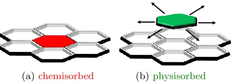
[image:4.612.190.422.383.468.2](a)chemisorbed (b)physisorbed
Figure 1: Possible molecular states. Molecules in their chemisorbed state (a) are locked in their position, while physisorbed molecules are free to diffuse on the hexagonal lattice (b).
We simulate the self-assembly of non-overlapping hexagonal molecules on a hexagonal
lattice in the NVT ensemble. On the lattice each molecule i can be in one of two possible
adsorption states si (as in Fig. 1): chemisorbed (si = chem) or physisorbed (si = phys) .
Each lattice site can be occupied by only one molecule.
Two adjacent molecules, i and j, interact with each other via the interaction parameter,
Eijside. When both molecules are in different adsorption states i.e. when si = sj, it is
assumed that the interaction is negligible and Eijside = 0. Molecules interact with the surface
Hamiltonian of the system is:
H =X
i
Esi
ads+ 1 2
X
i,j
Esi,sj
ij with i6=j (1)
where
Eijsi,sj =
Eijside if si =sj
0 otherwise
(2)
and Esi
ads is the adsorption energy for molecule i, which can be in either the physisorbed (Esi
ads =E phys
ads ) or chemisorbed states (E si
ads = Eadschem). The first summation is taken over all molecules and the second summation is only over adjacent molecules. All energies are in
units of kBT, wherekB is the Boltzmann constant.
At each simulation step a molecule is selected at random and either a chemisorbed/physisorbed
transition occurs or a translation to the next lattice site is attempted. Only one move can
be attempted at each simulation step. Only physisorbed molecules can translate to adjacent
sites. If a molecule is chemisorbed only a transition to a physisorbed state is possible. All the
attempted moves are accepted or rejected following the Metropolis acceptance probability.30
We do not account for rotations, thereforeEijside is constant for all the molecular orientations.
The system is composed of 1000 molecules interacting via the Hamiltonian in Eq. (1) on
a 50×50 hexagonal lattice with periodic boundary conditions, corresponding to a coverage
of 0.4. To verify the effect of the coverage, selected parameter combinations were also run
with 972 molecules on a 54×54 lattice corresponding to a coverage of 0.33.
A chain of 400 simulations is built, with each simulation consisting of 5,000,000
equilibra-tion steps followed by 5,000,000 producequilibra-tion steps. Every chain starts at 0.4kBT and every
successive simulation is run by decreasing the temperature by ∆kBT = 0.002 and using the
last configuration of the former simulation as starting configuration. The low temperature
configurations are then heated back to 0.4kBT following the same protocol. Each simulation
Eadschem= 0.0, E phys
ads =−0.5 E chem ads =E
phys
ads = 0.0 E chem
ads =−0.5, E phys ads = 0.0
E
side ij
=
−
0
.
5
E
side ij
=
0
.
0
E
side ij
=
0
.
5
(a) (b) (c)
(d) (e) (f)
[image:6.612.82.550.70.396.2](g) (h) (i)
Figure 2: Patterns formed at kBT = 0.002. Insets show an enlarged detail of each snapshot. Physisorbed (chemisorbed) molecules are shown as green (orange).
simulations run with the same parameter set. No hysteresis effects were observed, therefore,
in the next section we will discuss only the results obtained upon cooling.
We generalise our former study21by exploring a larger parameter spaceEadsphys = [−0.5,0.0],
Eadschem = [−0.5,0.0] and Eijside = [−0.5,0.5]. As we are interested in exploring trends, and
keeping in mind that all the energy parameters are in units of kBT and can therefore be
rescaled, only their ratio is important. Each parameter is chosen among 0, ±0.001, ±0.005,
±0.01, ±0.05, ±0.1,±0.5. By combining Eadsphys, Eadschem, Eijside we obtain 637 systems each
3. Results and Discussion
In the following, we first look at low temperature limiting cases. Then we look at the details
of the structural transitions encountered to produce the observed patterns. The behaviour
of the system is described by the heat capacity at constant volume
CV = (∆E)
2
kBT2
,
and several different order parameters:
(i) the fraction of physisorbed molecules,χphys,
(ii) the total number of neighbors of each molecule, Nneigh,
(iii) the number of chemisorbed neighbors of each chemisorbed molecule, Ncc,
(iv) the number of physisorbed neighbors of each physisorbed molecule, Npp,
(v) and the number of unlike neighbors
Npc =Ncp=Nneigh−Npp−Ncc
The peaks in the running standard deviations of these order parameters enables us to further
locate the locus of structural transitions. Finally, after characterising the observed defects on
the self-assembled structures, we collect our results in a number of phase diagrams associated
with the choice of parameters.
3.1 Low temperature phases
By first looking at few limiting cases, a number of low-temperature (kBT = 0.002) patterns
Strong, attractive molecule–molecule interactions with Eijside =−0.5 lead to packed
pat-terns (Fig. 2a-c). The molecules can be all physisorbed, for instance when the chemisorbed
interaction is switched off, as shown in Fig. 2a, or all chemisorbed when the physisorption
teraction is switched off, as shown in Fig. 2c. When both chemisorption and physisorption
in-teractions are set to zero, a single chemisorbed cluster is observed (Fig. 2b). This chemisorbed
configuration arises from the fact that molecules are not mobile in the chemisorbed state
while they can freely diffuse in the physisorbed state. When a first chemisorbed cluster
forms, further molecules from the physisorbed state can add to it and then be locked in their
position favouring a large packed chemisorbed pattern at low temperature.
When the molecule–molecule interaction is switched off, i.e. Eijside = 0.0, the system does
not pack, as shown in Figs. 2d-f. The system freezes in a disordered state whose adsorption
state of the frozen molecules depends on the relative strength of the adsorption energies
(Fig. 3). When Eadschem = Eadsphys half of the molecules are chemisorbed, and the rest are
physisorbed (Fig. 2e). When Eadsphys Eadschem = 0.0 they are all physisorbed (Fig. 2d) when
Eadschem Eadsphys = 0 they are all chemisorbed (Fig. 2f). In the case when Eadsphys and Eadschem
are both negative but much weaker (closer to zero) the number of physisorbed/chemisorbed
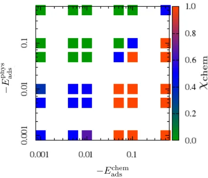
molecules depends on their respective interaction strength. For instance, whenEadschem= 0.001
and Eadsphys = 0.01 only 40% of the molecules are chemisorbed whereas when Eadschem = 0.01
and Eadsphys = 0.001 then 60% are chemisorbed (Fig. 3).
In the case of repulsive intermolecular interactions (for instance when Eijside = 0.5) we
would expect molecules to avoid occupying adjacent lattice sites. When the coverage is
greater than 13 (as is the case when the coverage is 0.4) we observe a number of strategies
to escape higher energy configurations. Depending on the physisorption and chemisorption
strength we observe the formation of:
• an ordered layer of physisorbed molecules with dislocations and defects in the form of
chemisorbed molecules whenEadsphys Eadschem= 0.0 (Fig. 2g),
1
−Echem
ads
−
E
ph
ys
[image:9.612.199.412.70.252.2]ads
Figure 3: Fraction of chemisorbed molecules as a function of Eadsphys and Eadschem forEijside = 0.0 atkBT = 0.002.
molecules when Eadsphys =Eadschem= 0.0 (Fig. 2h), and
• an ordered layer of chemisorbed molecules with dislocations and defects in the form of
physisorbed molecules when EadschemEadsphys = 0.0 (Fig. 2i).
If the coverage is below or equal to 0.33, we might expect to observe complete order.
Interestingly, whenEadsphys Eadschem= 0.0 (Fig. 4a) complete order is not achieved and defects
in the form of vacancies or insertions are present. It is the non-mobile chemisorption state
that causes these defects. Chemisorbed molecules would have to first become physisorbed
in order to migrate to a new adsorption site, but this process is hindered due to repulsive
intermolecular interactions between molecules in the same adsorption state. When Eadschem
Eadsphys = 0.0 (Fig. 4b), physisorbed molecules at defect sites can escape and freely diffuse to
fill all the vacancies enabling complete order to be reached.
The formation of defects can be better understood by observing their occurrence at fixed
values of adsorption energies along increasing values of Eijside (Fig. 5). Defects appear in
different forms, depending on the interplay among interactions. For instance, at Eadschem = −0.05, Eadsphys = −0.01, and going from Eijside = −0.05 to 0.00 first the packed structures
Eadschem= 0.0, E phys
ads =−0.5 E chem
ads =−0.5, E phys ads = 0.0
E
side ij
=
0
.
[image:10.612.168.444.71.161.2]5 (a) (b)
Figure 4: Patterns formed at kBT = 0.002. Physisorbed molecules (green), chemisorbed molecules (orange). At coverage 0.33. Structural defects are highlightd by black circles.
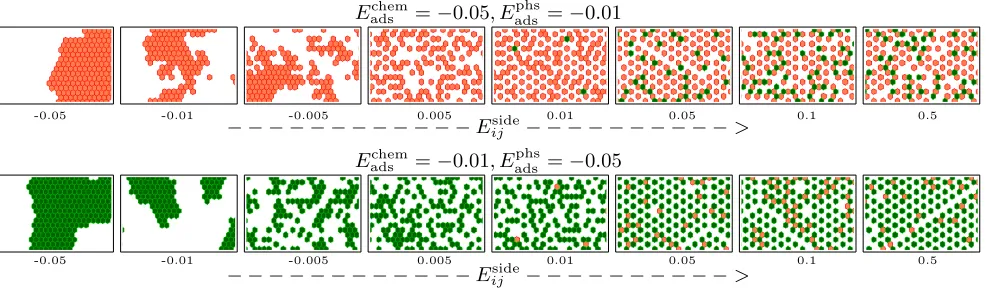
Eadschem=−0.05, E
phs
ads =−0.01
-0.05 -0.01 -0.005 0.005 0.01 0.05 0.1 0.5
− − − − − − − − − − − −Eside
ij − − − − − − − − − −>
Eadschem=−0.01, E
phs
ads =−0.05
-0.05 -0.01 -0.005 0.005 0.01 0.05 0.1 0.5
− − − − − − − − − − − −Eside
ij − − − − − − − − − −>
Figure 5: Defect formation in the patterns formed at fixed Eadschem and Eadsphys at 0.002kBT. Physisorbed (chemisorbed) molecules are shown in green (orange).
panels). When the side interactions are close to zero the structure is completely fragmented.
Fragmentation persists at 0.005 and defects of physisorbed molecules emerge at more positive
Eijside (0.01). The more repulsive the intermolecular interaction, the higher the number of
physisorption defects. When Eijside ∼ (−Eadschem) a new ordered state emerges with grain
boundary defects. When Eijside ≥ (−Eadschem) the grain boundaries increase and the patterns
again appear fragmented. A similar observation applies for the case in whichEadschem=−0.01
and Eadsphys = −0.05 (Fig. 5, bottom panels). However, when Eijside ≥ (−Eadsphys), the pattern
remains ordered with grain boundary and chemisorption defects.
3.2 Phase transitions
In this section we investigate the structures that emerge at different temperatures. By looking
[image:10.612.83.576.212.356.2]1
attractive side-side interactions
Cv (a.u.) Echem=0.0, Ephys=-0.5 0.2 0.4 0.6 0.8 1 X(dw) 1 23 45 N 1 23 45 N(0,0)
0 0.1 0.2 0.3 kT 1 23 45 N(1,1) Cv (a.u.) 0.2 0.4 0.6 0.8 1 2.2 2.4 2.6 2.8 0.5 1.0 1.5 2.0
0 0.1 0.2 0.3 kT 0.5 1.0 1.5 2.0 Cv (a.u.) 0.2 0.4 0.6 0.8 1 1.0 1.5 2.0 2.5 0.2 0.4 0.6 0.8
0 0.1 0.2 0.3 kT 0.2
0.4 0.6 0.8
q=-0.5 q=0.0 q=0.5
(a) (b) (c) (d) (e) (a) (b) (c) (d) (e) (a) (b) (c) (d) (e) A
P Cv (a.u.)
Echem=0.0, Ephys=0.0 0.2 0.4 0.6 0.8 1 X(dw) 1 23 45 N 1 23 45 N(0,0)
0 0.1 0.2 0.3 kT 1 23 45 N(1,1) Cv (a.u.) 0.2 0.4 0.6 0.8 1 2.2 2.4 2.6 2.8 0.5 1.0 1.5 2.0
0 0.1 0.2 0.3 kT 0.5 1.0 1.5 2.0 Cv (a.u.) 0.2 0.4 0.6 0.8 1 1.0 1.5 2.0 2.5 0.2 0.4 0.6 0.8
0 0.1 0.2 0.3 kT 0.1
0.20.3 0.40.5
q=-0.5 q=0.0 q=0.5
(g) (h) (i) (j) (k) (g) (h) (i) (j) (k) (g) (h) (i) (j) (k) Cv (a.u.) Echem=-0.5, Ephys=0.0 0.2 0.4 0.6 0.8 1 X(dw) 1 23 45 N 1 23 45 N(0,0)
0 0.1 0.2 0.3 kT 1 23 45 N(1,1) Cv (a.u.) 0.2 0.4 0.6 0.8 1 2.2 2.4 2.6 2.8 0.5 1.0 1.5 2.0
0 0.1 0.2 0.3 kT 0.5 1.0 1.5 2.0 Cv (a.u.) 0.2 0.4 0.6 0.8 1 1.0 1.5 2.0 2.5 0.2 0.4 0.6 0.8
0 0.1 0.2 0.3 kT 0.2
0.4 0.6 0.8
q=-0.5 q=0.0 q=0.5
(m) (n) (o) (p) (q) (m) (n) (o) (p) (q) (m) (n) (o) (p) (q) Cv (a.u.) Echem=0.0, Ephys=-0.5 0.5 1.0 1.5 N-N0-N11 01 23 45 N 01 23 45 N(0,0)
0 0.1 0.2 0.3 kT 01 23 45 N(1,1) Cv (a.u.) 0.5 1.0 1.5 2.2 2.4 2.6 2.8 0 0.5 1.0 1.5 2.0
0 0.1 0.2 0.3 kT 0 0.5 1.0 1.5 2.0 Cv (a.u.) 0.5 1.0 1.5 1.0 1.5 2.0 2.5 0 0.2 0.4 0.6 0.8
0 0.1 0.2 0.3 kT 0 0.2 0.4 0.6 0.8
q=-0.5 q=0.0 q=0.5
(a) (f) (c) (d) (e) (a) (f) (c) (d) (e) (a) (f) (c) (d) (e) A
P Cv (a.u.)
Echem=0.0, Ephys=0.0 0.5 1.0 1.5 N-N0-N1 01 23 45 N 01 23 45 N(0,0)
0 0.1 0.2 0.3 kT 01 23 45 N(1,1) Cv (a.u.) 0.5 1.0 1.5 2.2 2.4 2.6 2.8 0 0.5 1.0 1.5 2.0
0 0.1 0.2 0.3 kT 0 0.5 1.0 1.5 2.0 Cv (a.u.) 0.5 1.0 1.5 1.0 1.5 2.0 2.5 0 0.2 0.4 0.6 0.8
0 0.1 0.2 0.3 kT 0
0.1 0.20.3 0.40.5
q=-0.5 q=0.0 q=0.5
(f) (l) (h) (i) (j) (f) (l) (h) (i) (j) (f) (l) (h) (i) (j) Cv (a.u.) Echem=-0.5, Ephys=0.0 0.5 1.0 1.5 N-N0-N1 01 23 45 N 01 23 45 N(0,0)
0 0.1 0.2 0.3 kT 01 23 45 N(1,1) Cv (a.u.) 0.5 1.0 1.5 2.2 2.4 2.6 2.8 0 0.5 1.0 1.5 2.0
0 0.1 0.2 0.3 kT 0 0.5 1.0 1.5 2.0 Cv (a.u.) 0.5 1.0 1.5 1.0 1.5 2.0 2.5 0 0.2 0.4 0.6 0.8
0 0.1 0.2 0.3 kT 0 0.2 0.4 0.6 0.8
q=-0.5 q=0.0 q=0.5
(k) (r) (m) (n) (o) (k) (r) (m) (n) (o) (k) (r) (m) (n) (o) Cv (a.u.) Echem=0.0, Ephys=-0.5 0.2 0.4 0.6 0.8 1 X(dw) 1 23 45 N 1 23 45 N(0,0)
0 0.1 0.2 0.3 kT 1 23 45 N(1,1) Cv (a.u.) 0.2 0.4 0.6 0.8 1 2.2 2.4 2.6 2.8 0.5 1.0 1.5 2.0
0 0.1 0.2 0.3 kT 0.5 1.0 1.5 2.0 Cv (a.u.) 0.2 0.4 0.6 0.8 1 1.0 1.5 2.0 2.5 0.2 0.4 0.6 0.8
0 0.1 0.2 0.3 kT 0.2
0.4 0.6 0.8
q=-0.5 q=0.0 q=0.5
(a) (b) (c) (d) (e) (a) (b) (c) (d) (e) (a) (b) (c) (d) (e) A
P Cv (a.u.)
Echem=0.0, Ephys=0.0 0.2 0.4 0.6 0.8 1 X(dw) 1 23 45 N 1 23 45 N(0,0)
0 0.1 0.2 0.3 kT 1 23 45 N(1,1) Cv (a.u.) 0.2 0.4 0.6 0.8 1 2.2 2.4 2.6 2.8 0.5 1.0 1.5 2.0
0 0.1 0.2 0.3 kT 0.5 1.0 1.5 2.0 Cv (a.u.) 0.2 0.4 0.6 0.8 1 1.0 1.5 2.0 2.5 0.2 0.4 0.6 0.8
0 0.1 0.2 0.3 kT 0.1
0.20.3 0.40.5
q=-0.5 q=0.0 q=0.5
(g) (h) (i) (j) (k) (g) (h) (i) (j) (k) (g) (h) (i) (j) (k) Cv (a.u.) Echem=-0.5, Ephys=0.0 0.2 0.4 0.6 0.8 1 X(dw) 1 23 45 N 1 23 45 N(0,0)
0 0.1 0.2 0.3 kT 1 23 45 N(1,1) Cv (a.u.) 0.2 0.4 0.6 0.8 1 2.2 2.4 2.6 2.8 0.5 1.0 1.5 2.0
0 0.1 0.2 0.3 kT 0.5 1.0 1.5 2.0 Cv (a.u.) 0.2 0.4 0.6 0.8 1 1.0 1.5 2.0 2.5 0.2 0.4 0.6 0.8
0 0.1 0.2 0.3 kT 0.2
0.4 0.6 0.8
q=-0.5 q=0.0 q=0.5
(m) (n) (o) (p) (q) (m) (n) (o) (p) (q) (m) (n) (o) (p) (q)
kBT kBT kBT
Eadschem= 0.0 Eadschem= 0.0 Echemads =−0.5 Eadsphys=−0.5 Eadsphys= 0.0 Eadsphys= 0.0
[image:11.612.183.430.73.354.2]N cp χph ys N pp N cc N neigh
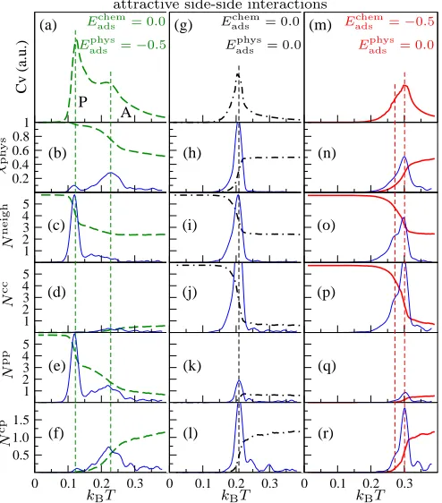
Figure 6: Self-assembly for attractive intermolecular interactions with Eijside = −0.5, corre-sponding to the low temperature phases in Fig. 2a-c. The top panels show the variation of CV in arbitrary units (a.u.) with temperature. The lower panels show running averages (calculated over 10 points) of order parameters with temperature. Also indicated in blue solid lines are the respective running standard deviations (calculated over 10 points) and 10×magnified.
the sequence of structural transitions that lead to the observed low temperature patterns.
The structures encountered can be further characterised by a number of order parameters
defined earlier: χphys, Nneigh, Ncc, Npp, and Ncp (Fig. 6-8).
3.2.1 Attractive intermolecular interactions For attractive intermolecular
inter-actions with Eadschem = 0.0 and Eadsphys = Eijside = −0.5, leading to the zero temperature
ph-ysisorbed packed pattern of Fig. 2a, two major transitions can be observed (Fig. 6a-f). The
first is a high temperature physisorption/chemisorption transition characterised by a peak in
CV (Fig. 6a), and associated with a rapid variation in χphys (Fig. 6b), no large variations in
Nneigh (Fig. 6c) andNcc (Fig. 6d), and a smooth variation inNpp(Fig. 6e) andNcp (Fig. 6f)
which is associated with a rapid change in Nneigh andNpp (Fig. 6c,e). The low temperature
value of Npp, which is close to its maximum value of 6, indicates the packing of the system
in a physisorbed state.
The case leading to the chemisorbed pattern of Fig. 2b follows a different route (Fig.
6g-l). In this case, the molecules do not interact with the surface (Eadschem = Eadsphys = 0.0) but
have attractive intermolecular interactions between molecules in the same adsorption state
(Eijside = −0.5). Only one sharp CV peak is present and physisorption/chemisorption and
packing transitions both take place at the same temperature, as shown in Fig. 6 g-l.
Inter-estingly, even though there is no energetic preference with respect to the adsorption state,
the molecules pack in a chemisorbed state, which is an effect of their arrested translational
mobility in that phase.
When Eadsphys = 0.0 and Eadschem=Eijside =−0.5 (Fig. 6m-r), thenCV exhibits a main peak
and a weak shoulder as shown in Fig. 6m. The shoulder is the low temperature packing
peak, now at 0.27kBT. The higher temperature main peak at 0.30kBT is the
physisorp-tion/chemisorption transition. Here all the order parameters sharply decreases (Fig. 6n-r)
with only Npp going to zero (Fig. 6q), while χphys (Fig. 6n) and Ncp (Fig. 6r) continues to
decrease and Nneigh (Fig. 6o) and Ncc (Fig. 6p) continues to increase at both temperatures.
The low temperature structure is once again a chemisorbed packed pattern (Fig. 2c).
3.2.2 Zero intermolecular interactions When the intermolecular interactions are
set to zero (Eijside = 0) leading to the disordered patterns of Fig. 2d-f, there appears to be a
single structural transition only when the molecule–surface interaction is active (Fig. 7a-r).
When Eadschem = 0.0 and Eadsphys = −0.5 there is a large peak in CV (Fig. 7a). This is a
physisorption/chemisorption transition leading to all molecules in their favoured physisorbed
state (Fig. 7b). Packing, of course, does not take place andNneigh is constant with
tempera-ture (Fig. 7c). As the temperatempera-ture decreases, the number of like neighbors in the unfavoured
favoured state (Fig. 7e). Also the number of unlike neighbors drops to zero (Fig. 7f).
As expected, when all the interactions are set to zero, no transition is observed, all
the order parameters are constant along the temperature (Fig. 7g-l) and the system stays
disordered.
On the other hand, in the scenario in which Eadschem=−0.5 and Eadsphys = 0.0 the observed
large peak in the CV (Fig. 7m) is once again associated with a physisorption/chemisorption
transition leading to all molecules in their favoured adsorption state, which in this case is
chemisorbed (Fig. 7n). As the molecules do not interact with each other, packing still does
not take place as highlighted by the constant values ofNneigh (Fig. 7o). As the temperature
decreases the number of like neighbors in the favoured adsorption state increases (Fig. 7p)
while the number of like neighbours decreases in the unfavoured state (Fig. 7q), and the
number of unlike neighbors drops to zero (Fig. 7r).
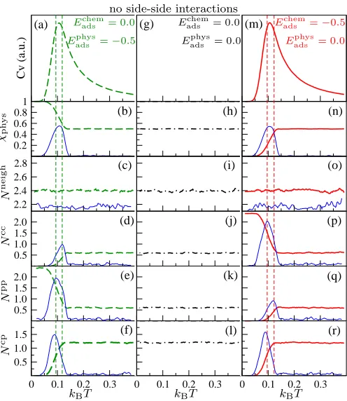
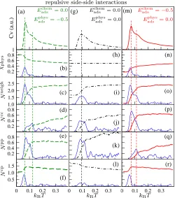
3.2.3 Repulsive intermolecular interactions Finally, we present the self-assembly
when the intermolecular interactions are repulsive (Eijside = 0.5, Fig. 2g-i) and molecules
occupying adjacent lattice sites will attempt to minimise repulsive interactions by minimising
the number of neighbors in the same adsorption state (Fig. 8a-r). When the physisorption
state is energetically favorable, for instance with Eadschem = 0.0 and Eadsphys =−0.5, decreasing
the temperature first shows a shoulder on the main CV peak at ≈0.12kBT (Fig. 8a) with a
minimal variation in χphys (Fig. 8b), the onset of Nneigh drop (Fig. 8c), and a slow decrease
inNcc (Fig. 8d).
The main peak inCV at lower temperature of≈0.06kBT (Fig. 8a) corresponds to a more
significant physisorption/chemisorption transition (Fig. 8b). There is a decrease in the total
number of neighbors,Npp (Fig. 8e). Below this temperature Ncc (Fig. 8d) and Npp (Fig. 8e)
fall to zero leaving only unlike neighbours (Fig. 8f).
When both physisorbed and chemisorbed adsorption energies are zero, there is only one
1
no side-side interactions
Cv (a.u.) Echem=0.0, Ephys=-0.5 0.2 0.4 0.6 0.8 1 X(dw) 1 23 45 N 1 23 45 N(0,0)
0 0.1 0.2 0.3 kT 1 23 45 N(1,1) Cv (a.u.) 0.2 0.4 0.6 0.8 1 2.2 2.4 2.6 2.8 0.5 1.0 1.5 2.0
0 0.1 0.2 0.3 kT 0.5 1.0 1.5 2.0 Cv (a.u.) 0.2 0.4 0.6 0.8 1 1.0 1.5 2.0 2.5 0.2 0.4 0.6 0.8
0 0.1 0.2 0.3 kT 0.2
0.4 0.6 0.8
q=-0.5 q=0.0 q=0.5
(a) (b) (c) (d) (e) (a) (b) (c) (d) (e) (a) (b) (c) (d) (e) A P Cv (a.u.) Echem=0.0, Ephys=-0.5 0.2 0.4 0.6 0.8 1 X(dw) 1 2 3 4 5 N 1 2 3 4 5 N(0,0)
0 0.1 0.2 0.3 kT 1 2 3 4 5 N(1,1) Cv (a.u.) 0.2 0.4 0.6 0.8 1 2.2 2.4 2.6 2.8 0.5 1.0 1.5 2.0
0 0.1 0.2 0.3 kT 0.5 1.0 1.5 2.0 Cv (a.u.) 0.2 0.4 0.6 0.8 1 1.0 1.5 2.0 2.5 0.2 0.4 0.6 0.8
0 0.1 0.2 0.3 kT 0.2
0.4 0.6 0.8
q=-0.5 q=0.0 q=0.5
(a) (b) (c) (d) (e) (a) (b) (c) (d) (e) (a) (b) (c) (d) (e) A
P Cv (a.u.)
Echem=0.0, Ephys=0.0 0.2 0.4 0.6 0.8 1 X(dw) 1 2 3 4 5 N 1 2 3 4 5 N(0,0)
0 0.1 0.2 0.3 kT 1 2 3 4 5 N(1,1) Cv (a.u.) 0.2 0.4 0.6 0.8 1 2.2 2.4 2.6 2.8 0.5 1.0 1.5 2.0
0 0.1 0.2 0.3 kT 0.5 1.0 1.5 2.0 Cv (a.u.) 0.2 0.4 0.6 0.8 1 1.0 1.5 2.0 2.5 0.2 0.4 0.6 0.8
0 0.1 0.2 0.3 kT 0.1 0.2 0.3 0.4 0.5
q=-0.5 q=0.0 q=0.5
(g) (h) (i) (j) (k) (g) (h) (i) (j) (k) (g) (h) (i) (j) (k) Cv (a.u.) Echem=-0.5, Ephys=0.0 0.2 0.4 0.6 0.8 1 X(dw) 1 2 3 4 5 N 1 2 3 4 5 N(0,0)
0 0.1 0.2 0.3 kT 1 2 3 4 5 N(1,1) Cv (a.u.) 0.2 0.4 0.6 0.8 1 2.2 2.4 2.6 2.8 0.5 1.0 1.5 2.0
0 0.1 0.2 0.3 kT 0.5 1.0 1.5 2.0 Cv (a.u.) 0.2 0.4 0.6 0.8 1 1.0 1.5 2.0 2.5 0.2 0.4 0.6 0.8
0 0.1 0.2 0.3 kT 0.2
0.4 0.6 0.8
q=-0.5 q=0.0 q=0.5
(m) (n) (o) (p) (q) (m) (n) (o) (p) (q) (m) (n) (o) (p) (q) Cv (a.u.) Echem=0.0, Ephys=-0.5 0.5 1.0 1.5 N-N0-N11 01 23 45 N 01 23 45 N(0,0)
0 0.1 0.2 0.3 kT 01 23 45 N(1,1) Cv (a.u.) 0.5 1.0 1.5 2.2 2.4 2.6 2.8 0 0.5 1.0 1.5 2.0
0 0.1 0.2 0.3 kT 0 0.5 1.0 1.5 2.0 Cv (a.u.) 0.5 1.0 1.5 1.0 1.5 2.0 2.5 0 0.2 0.4 0.6 0.8
0 0.1 0.2 0.3 kT 0 0.2 0.4 0.6 0.8
q=-0.5 q=0.0 q=0.5
(a) (f) (c) (d) (e) (a) (f) (c) (d) (e) (a) (f) (c) (d) (e) A P Cv (a.u.) Echem=0.0, Ephys=-0.5 0.5 1.0 1.5 N-N0-N11 01 2 3 4 5 N 01 2 3 4 5 N(0,0)
0 0.1 0.2 0.3 kT 01 2 3 4 5 N(1,1) Cv (a.u.) 0.5 1.0 1.5 2.2 2.4 2.6 2.8 0 0.5 1.0 1.5 2.0
0 0.1 0.2 0.3 kT 0 0.5 1.0 1.5 2.0 Cv (a.u.) 0.5 1.0 1.5 1.0 1.5 2.0 2.5 0 0.2 0.4 0.6 0.8
0 0.1 0.2 0.3 kT 0 0.2 0.4 0.6 0.8
q=-0.5 q=0.0 q=0.5
(a) (f) (c) (d) (e) (a) (f) (c) (d) (e) (a) (f) (c) (d) (e) A
P Cv (a.u.)
Echem=0.0, Ephys=0.0 0.5 1.0 1.5 N-N0-N1 01 2 3 4 5 N 01 2 3 4 5 N(0,0)
0 0.1 0.2 0.3 kT 01 2 3 4 5 N(1,1) Cv (a.u.) 0.5 1.0 1.5 2.2 2.4 2.6 2.8 0 0.5 1.0 1.5 2.0
0 0.1 0.2 0.3 kT 0 0.5 1.0 1.5 2.0 Cv (a.u.) 0.5 1.0 1.5 1.0 1.5 2.0 2.5 0 0.2 0.4 0.6 0.8
0 0.1 0.2 0.3 kT 0 0.1 0.2 0.3 0.4 0.5
q=-0.5 q=0.0 q=0.5
(f) (l) (h) (i) (j) (f) (l) (h) (i) (j) (f) (l) (h) (i) (j) Cv (a.u.) Echem=-0.5, Ephys=0.0 0.5 1.0 1.5 N-N0-N1 01 2 3 4 5 N 01 2 3 4 5 N(0,0)
0 0.1 0.2 0.3 kT 01 2 3 4 5 N(1,1) Cv (a.u.) 0.5 1.0 1.5 2.2 2.4 2.6 2.8 0 0.5 1.0 1.5 2.0
0 0.1 0.2 0.3 kT 0 0.5 1.0 1.5 2.0 Cv (a.u.) 0.5 1.0 1.5 1.0 1.5 2.0 2.5 0 0.2 0.4 0.6 0.8
0 0.1 0.2 0.3 kT 0 0.2 0.4 0.6 0.8
q=-0.5 q=0.0 q=0.5
(k) (r) (m) (n) (o) (k) (r) (m) (n) (o) (k) (r) (m) (n) (o) Cv (a.u.) Echem=0.0, Ephys=-0.5 0.2 0.4 0.6 0.8 1 X(dw) 1 23 45 N 1 23 45 N(0,0)
0 0.1 0.2 0.3 kT 1 23 45 N(1,1) Cv (a.u.) 0.2 0.4 0.6 0.8 1 2.2 2.4 2.6 2.8 0.5 1.0 1.5 2.0
0 0.1 0.2 0.3 kT 0.5 1.0 1.5 2.0 Cv (a.u.) 0.2 0.4 0.6 0.8 1 1.0 1.5 2.0 2.5 0.2 0.4 0.6 0.8
0 0.1 0.2 0.3 kT 0.2
0.4 0.6 0.8
q=-0.5 q=0.0 q=0.5
(a) (b) (c) (d) (e) (a) (b) (c) (d) (e) (a) (b) (c) (d) (e) A P Cv (a.u.) Echem=0.0, Ephys=-0.5 0.2 0.4 0.6 0.8 1 X(dw) 1 2 3 4 5 N 1 2 3 4 5 N(0,0)
0 0.1 0.2 0.3 kT 1 2 3 4 5 N(1,1) Cv (a.u.) 0.2 0.4 0.6 0.8 1 2.2 2.4 2.6 2.8 0.5 1.0 1.5 2.0
0 0.1 0.2 0.3 kT 0.5 1.0 1.5 2.0 Cv (a.u.) 0.2 0.4 0.6 0.8 1 1.0 1.5 2.0 2.5 0.2 0.4 0.6 0.8
0 0.1 0.2 0.3 kT 0.2
0.4 0.6 0.8
q=-0.5 q=0.0 q=0.5
(a) (b) (c) (d) (e) (a) (b) (c) (d) (e) (a) (b) (c) (d) (e) A
P Cv (a.u.)
Echem=0.0, Ephys=0.0 0.2 0.4 0.6 0.8 1 X(dw) 1 2 3 4 5 N 1 2 3 4 5 N(0,0)
0 0.1 0.2 0.3 kT 1 2 3 4 5 N(1,1) Cv (a.u.) 0.2 0.4 0.6 0.8 1 2.2 2.4 2.6 2.8 0.5 1.0 1.5 2.0
0 0.1 0.2 0.3 kT 0.5 1.0 1.5 2.0 Cv (a.u.) 0.2 0.4 0.6 0.8 1 1.0 1.5 2.0 2.5 0.2 0.4 0.6 0.8
0 0.1 0.2 0.3 kT 0.1 0.2 0.3 0.4 0.5
q=-0.5 q=0.0 q=0.5
(g) (h) (i) (j) (k) (g) (h) (i) (j) (k) (g) (h) (i) (j) (k) Cv (a.u.) Echem=-0.5, Ephys=0.0 0.2 0.4 0.6 0.8 1 X(dw) 1 2 3 4 5 N 1 2 3 4 5 N(0,0)
0 0.1 0.2 0.3 kT 1 2 3 4 5 N(1,1) Cv (a.u.) 0.2 0.4 0.6 0.8 1 2.2 2.4 2.6 2.8 0.5 1.0 1.5 2.0
0 0.1 0.2 0.3 kT 0.5 1.0 1.5 2.0 Cv (a.u.) 0.2 0.4 0.6 0.8 1 1.0 1.5 2.0 2.5 0.2 0.4 0.6 0.8
0 0.1 0.2 0.3 kT 0.2
0.4 0.6 0.8
q=-0.5 q=0.0 q=0.5
(m) (n) (o) (p) (q) (m) (n) (o) (p) (q) (m) (n) (o) (p) (q)
kBT kBT kBT
Eadschem= 0.0 Echemads = 0.0 Eadschem=−0.5 Ephysads =−0.5 Eadsphys= 0.0 Ephysads = 0.0
[image:14.612.182.430.69.355.2]N cp χph ys N pp N cc N neigh
Figure 7: Self-assembly for zero intermolecular interactions with Eijside = 0.0, corresponding to the low temperature phases in Fig. 2 d-f. The top panels show the variation of CV in arbitrary units (a.u.) with temperature. The lower panels show running averages (calculated over 10 points) of order parameters with temperature. Also indicated in blue solid lines are the respective running standard deviations (calculated over 10 points) and 10× magnified.
to a decrease in Nneigh which goes to 0.16 (Fig. 8i) and in Ncc (Fig. 8j) and Npp (Fig. 8k)
both going to zero. A slight increase in unlike neighbours Ncp is also observed (Fig. 8l).
The order parameter standard deviations are observed to be double peaks (Fig. 8i-l). In this
case, the low temperature structure has chains of alternating physisorbed and chemisorbed
molecules (Fig. 2h).
Two unresolved peaks on the CV are also observed when the most favourable adsorption
state is chemisorbed, for instance with Eadschem=−0.5 and Eadsphys = 0.0 (Fig. 8m). A drop in
χphys (Fig. 8n) is associated only with the low temperature main transition at 0.11kBT, while
Nneigh (Fig. 8o) and Ncc (Fig. 8p) tend to drop at both the temperatures identified by the
CV peaks. Npp is minimised at 0.11kBT (Fig. 8q) while the onset of Ncp drop is observed
1
repulsive side-side interactions
Cv (a.u.) Echem=0.0, Ephys=-0.5 0.2 0.4 0.6 0.8 1 X(dw) 1 23 45 N 1 23 45 N(0,0)
0 0.1 0.2 0.3 kT 1 23 45 N(1,1) Cv (a.u.) 0.2 0.4 0.6 0.8 1 2.2 2.4 2.6 2.8 0.5 1.0 1.5 2.0
0 0.1 0.2 0.3 kT 0.5 1.0 1.5 2.0 Cv (a.u.) 0.2 0.4 0.6 0.8 1 1.0 1.5 2.0 2.5 0.2 0.4 0.6 0.8
0 0.1 0.2 0.3 kT 0.2
0.4 0.6 0.8
q=-0.5 q=0.0 q=0.5
(a) (b) (c) (d) (e) (a) (b) (c) (d) (e) (a) (b) (c) (d) (e) A P Cv (a.u.) Echem=0.0, Ephys=-0.5 0.2 0.4 0.6 0.8 1 X(dw) 1 23 45 N 1 23 45 N(0,0)
0 0.1 0.2 0.3 kT 1 23 45 N(1,1) Cv (a.u.) 0.2 0.4 0.6 0.8 1 2.2 2.4 2.6 2.8 0.5 1.0 1.5 2.0
0 0.1 0.2 0.3 kT 0.5 1.0 1.5 2.0 Cv (a.u.) 0.2 0.4 0.6 0.8 1 1.0 1.5 2.0 2.5 0.2 0.4 0.6 0.8
0 0.1 0.2 0.3 kT 0.2
0.4 0.6 0.8
q=-0.5 q=0.0 q=0.5
(a) (b) (c) (d) (e) (a) (b) (c) (d) (e) (a) (b) (c) (d) (e) A
P Cv (a.u.)
Echem=0.0, Ephys=0.0 0.2 0.4 0.6 0.8 1 X(dw) 1 23 45 N 1 23 45 N(0,0)
0 0.1 0.2 0.3 kT 1 23 45 N(1,1) Cv (a.u.) 0.2 0.4 0.6 0.8 1 2.2 2.4 2.6 2.8 0.5 1.0 1.5 2.0
0 0.1 0.2 0.3 kT 0.5 1.0 1.5 2.0 Cv (a.u.) 0.2 0.4 0.6 0.8 1 1.0 1.5 2.0 2.5 0.2 0.4 0.6 0.8
0 0.1 0.2 0.3 kT 0.1 0.2 0.3 0.4 0.5
q=-0.5 q=0.0 q=0.5
(g) (h) (i) (j) (k) (g) (h) (i) (j) (k) (g) (h) (i) (j) (k) Cv (a.u.) Echem=-0.5, Ephys=0.0 0.2 0.4 0.6 0.8 1 X(dw) 1 23 45 N 1 23 45 N(0,0)
0 0.1 0.2 0.3 kT 1 23 45 N(1,1) Cv (a.u.) 0.2 0.4 0.6 0.8 1 2.2 2.4 2.6 2.8 0.5 1.0 1.5 2.0
0 0.1 0.2 0.3 kT 0.5 1.0 1.5 2.0 Cv (a.u.) 0.2 0.4 0.6 0.8 1 1.0 1.5 2.0 2.5 0.2 0.4 0.6 0.8
0 0.1 0.2 0.3 kT 0.2
0.4 0.6 0.8
q=-0.5 q=0.0 q=0.5
(m) (n) (o) (p) (q) (m) (n) (o) (p) (q) (m) (n) (o) (p) (q) Cv (a.u.) Echem=0.0, Ephys=-0.5 0.5 1.0 1.5 N-N0-N11 01 23 45 N 01 23 45 N(0,0)
0 0.1 0.2 0.3 kT 01 23 45 N(1,1) Cv (a.u.) 0.5 1.0 1.5 2.2 2.4 2.6 2.8 0 0.5 1.0 1.5 2.0
0 0.1 0.2 0.3 kT 0 0.5 1.0 1.5 2.0 Cv (a.u.) 0.5 1.0 1.5 1.0 1.5 2.0 2.5 0 0.2 0.4 0.6 0.8
0 0.1 0.2 0.3 kT 0 0.2 0.4 0.6 0.8
q=-0.5 q=0.0 q=0.5
(a) (f) (c) (d) (e) (a) (f) (c) (d) (e) (a) (f) (c) (d) (e) A P Cv (a.u.) Echem=0.0, Ephys=-0.5 0.5 1.0 1.5 N-N0-N11 01 23 45 N 01 23 45 N(0,0)
0 0.1 0.2 0.3 kT 01 23 45 N(1,1) Cv (a.u.) 0.5 1.0 1.5 2.2 2.4 2.6 2.8 0 0.5 1.0 1.5 2.0
0 0.1 0.2 0.3 kT 0 0.5 1.0 1.5 2.0 Cv (a.u.) 0.5 1.0 1.5 1.0 1.5 2.0 2.5 0 0.2 0.4 0.6 0.8
0 0.1 0.2 0.3 kT 0 0.2 0.4 0.6 0.8
q=-0.5 q=0.0 q=0.5
(a) (f) (c) (d) (e) (a) (f) (c) (d) (e) (a) (f) (c) (d) (e) A
P Cv (a.u.)
Echem=0.0, Ephys=0.0 0.5 1.0 1.5 N-N0-N1 01 23 45 N 01 23 45 N(0,0)
0 0.1 0.2 0.3 kT 01 23 45 N(1,1) Cv (a.u.) 0.5 1.0 1.5 2.2 2.4 2.6 2.8 0 0.5 1.0 1.5 2.0
0 0.1 0.2 0.3 kT 0 0.5 1.0 1.5 2.0 Cv (a.u.) 0.5 1.0 1.5 1.0 1.5 2.0 2.5 0 0.2 0.4 0.6 0.8
0 0.1 0.2 0.3 kT 0 0.1 0.2 0.3 0.4 0.5
q=-0.5 q=0.0 q=0.5
(f) (l) (h) (i) (j) (f) (l) (h) (i) (j) (f) (l) (h) (i) (j) Cv (a.u.) Echem=-0.5, Ephys=0.0 0.5 1.0 1.5 N-N0-N1 01 23 45 N 01 23 45 N(0,0)
0 0.1 0.2 0.3 kT 01 23 45 N(1,1) Cv (a.u.) 0.5 1.0 1.5 2.2 2.4 2.6 2.8 0 0.5 1.0 1.5 2.0
0 0.1 0.2 0.3 kT 0 0.5 1.0 1.5 2.0 Cv (a.u.) 0.5 1.0 1.5 1.0 1.5 2.0 2.5 0 0.2 0.4 0.6 0.8
0 0.1 0.2 0.3 kT 0 0.2 0.4 0.6 0.8
q=-0.5 q=0.0 q=0.5
(k) (r) (m) (n) (o) (k) (r) (m) (n) (o) (k) (r) (m) (n) (o) Cv (a.u.) Echem=0.0, Ephys=-0.5 0.2 0.4 0.6 0.8 1 X(dw) 1 23 45 N 1 23 45 N(0,0)
0 0.1 0.2 0.3 kT 1 23 45 N(1,1) Cv (a.u.) 0.2 0.4 0.6 0.8 1 2.2 2.4 2.6 2.8 0.5 1.0 1.5 2.0
0 0.1 0.2 0.3 kT 0.5 1.0 1.5 2.0 Cv (a.u.) 0.2 0.4 0.6 0.8 1 1.0 1.5 2.0 2.5 0.2 0.4 0.6 0.8
0 0.1 0.2 0.3 kT 0.2
0.4 0.6 0.8
q=-0.5 q=0.0 q=0.5
(a) (b) (c) (d) (e) (a) (b) (c) (d) (e) (a) (b) (c) (d) (e) A P Cv (a.u.) Echem=0.0, Ephys=-0.5 0.2 0.4 0.6 0.8 1 X(dw) 1 23 45 N 1 23 45 N(0,0)
0 0.1 0.2 0.3 kT 1 23 45 N(1,1) Cv (a.u.) 0.2 0.4 0.6 0.8 1 2.2 2.4 2.6 2.8 0.5 1.0 1.5 2.0
0 0.1 0.2 0.3 kT 0.5 1.0 1.5 2.0 Cv (a.u.) 0.2 0.4 0.6 0.8 1 1.0 1.5 2.0 2.5 0.2 0.4 0.6 0.8
0 0.1 0.2 0.3 kT 0.2
0.4 0.6 0.8
q=-0.5 q=0.0 q=0.5
(a) (b) (c) (d) (e) (a) (b) (c) (d) (e) (a) (b) (c) (d) (e) A
P Cv (a.u.)
Echem=0.0, Ephys=0.0 0.2 0.4 0.6 0.8 1 X(dw) 1 23 45 N 1 23 45 N(0,0)
0 0.1 0.2 0.3 kT 1 23 45 N(1,1) Cv (a.u.) 0.2 0.4 0.6 0.8 1 2.2 2.4 2.6 2.8 0.5 1.0 1.5 2.0
0 0.1 0.2 0.3 kT 0.5 1.0 1.5 2.0 Cv (a.u.) 0.2 0.4 0.6 0.8 1 1.0 1.5 2.0 2.5 0.2 0.4 0.6 0.8
0 0.1 0.2 0.3 kT 0.1 0.2 0.3 0.4 0.5
q=-0.5 q=0.0 q=0.5
(g) (h) (i) (j) (k) (g) (h) (i) (j) (k) (g) (h) (i) (j) (k) Cv (a.u.) Echem=-0.5, Ephys=0.0 0.2 0.4 0.6 0.8 1 X(dw) 1 23 45 N 1 23 45 N(0,0)
0 0.1 0.2 0.3 kT 1 23 45 N(1,1) Cv (a.u.) 0.2 0.4 0.6 0.8 1 2.2 2.4 2.6 2.8 0.5 1.0 1.5 2.0
0 0.1 0.2 0.3 kT 0.5 1.0 1.5 2.0 Cv (a.u.) 0.2 0.4 0.6 0.8 1 1.0 1.5 2.0 2.5 0.2 0.4 0.6 0.8
0 0.1 0.2 0.3 kT 0.2
0.4 0.6 0.8
q=-0.5 q=0.0 q=0.5
(m) (n) (o) (p) (q) (m) (n) (o) (p) (q) (m) (n) (o) (p) (q)
kBT kBT kBT
Echem
ads = 0.0 Echemads = 0.0 Eadschem=−0.5 Eadsphys=−0.5 Eadsphys= 0.0 Eadsphys= 0.0
[image:15.612.183.433.72.355.2]N cp χph ys N pp N cc N neigh
Figure 8: Self-assembly for repulsive intermolecular interactions with Eijside = 0.5, corre-sponding to the low temperature phases in Fig. 2g-i. The top panels show the variation of CV in arbitrary units (a.u.) with temperature. The lower panels show running averages (calculated over 10 points) of order parameters with temperature. Also indicated in blue solid lines are the respective running standard deviations (calculated over 10 points) and 10×magnified.
3.3 Phase diagrams
The observed phases and defect patterns enable the entire configurational space to be
char-acterised, and in Fig. 9 the observed low temperature patterns are schematised into a series
of two-dimensionalEadschemvsEadsphys phase diagrams. Each phase diagram is characterised by a
different intermolecular interaction strengthEijside (for molecules are in the same adsorption
state, see Eq. 2). In these plots an inverse logarithmic scale has been employed for clarity.
Attractive intermolecular interactions that are stronger or equal to the physisorption or
chemisorption interactions always lead to packing in the form of a large ordered cluster. In
the majority of cases all molecules are chemisorbed, which is due to no translation in the
1 1 1 0 0.001 0.01 0.1 -E(phys) 0 0.001 0.01 0.1 -E(chem) E(ij)=-0.5 0 0.001 0.01 0.1 -E(phys) 0 0.001 0.01 0.1 -E(chem) E(ij)=-0.05 0 0.001 0.01 0.1 -E(phys) 0 0.001 0.01 0.1 -E(chem) E(ij)=0.0 0 0.001 0.01 0.1 -E(phys) 0 0.001 0.01 0.1 -E(chem) E(ij)=0.05 0 0.001 0.01 0.1 -E(phys) 0 0.001 0.01 0.1 -E(chem) E(ij)=0.5
(a) (b) (c)
(d) (e) // // // // // \\ \\ \\ \\ \\ 1 0 0.001 0.01 0.1 -E(phys) 0 0.001 0.01 0.1 -E(chem) E(ij)=-0.5 0 0.001 0.01 0.1 -E(phys) 0 0.001 0.01 0.1 -E(chem) E(ij)=-0.05 0 0.001 0.01 0.1 -E(phys) 0 0.001 0.01 0.1 -E(chem) E(ij)=0.0 0 0.001 0.01 0.1 -E(phys) 0 0.001 0.01 0.1 -E(chem) E(ij)=0.05 0 0.001 0.01 0.1 -E(phys) 0 0.001 0.01 0.1 -E(chem) E(ij)=0.5
(a) (b) (c)
(d) (e) // // // // // \\ \\ \\ \\ \\ 1 1 0 0.001 0.01 0.1 -E(phys) 0 0.001 0.01 0.1 -E(chem) E(ij)=-0.5 0 0.001 0.01 0.1 -E(phys) 0 0.001 0.01 0.1 -E(chem) E(ij)=-0.05 0 0.001 0.01 0.1 -E(phys) 0 0.001 0.01 0.1 -E(chem) E(ij)=0.0 0 0.001 0.01 0.1 -E(phys) 0 0.001 0.01 0.1 -E(chem) E(ij)=0.05 0 0.001 0.01 0.1 -E(phys) 0 0.001 0.01 0.1 -E(chem) E(ij)=0.5
(a) (b) (c)
(d) (e) // // // // // \\ \\ \\ \\ \\ 1 0 0.001 0.01 0.1 -E(phys) 0 0.001 0.01 0.1 -E(chem) E(ij)=-0.5 0 0.001 0.01 0.1 -E(phys) 0 0.001 0.01 0.1 -E(chem) E(ij)=-0.05 0 0.001 0.01 0.1 -E(phys) 0 0.001 0.01 0.1 -E(chem) E(ij)=0.0 0 0.001 0.01 0.1 -E(phys) 0 0.001 0.01 0.1 -E(chem) E(ij)=0.05 0 0.001 0.01 0.1 -E(phys) 0 0.001 0.01 0.1 -E(chem) E(ij)=0.5
(a) (b) (c)
(d) (e) // // // // // \\ \\ \\ \\ \\ Eside
ij =−0.5 Eijside = −0.05 Eijside = −0.0
Eside
ij = 0.05 Eijside = 005
−Eadsphys −Ephysads −Eadsphys
−Eadsphys −Eadsphys
[image:16.612.82.576.74.461.2]− E c hem ads − E c hem ads − E c hem ads − E c hem ads − E c hem ads
Figure 9: Phase behavior at fixedEijsideat 0.002kBT for different physisorbed and chemisorbed interactions. Physisorbed (chemisorbed) molecules are shown in green (orange).
molecules are physisorbed. In the particular cases explored in Fig. 9a this is observed only
when Eadsphys =−0.5 and Eadschem≤ −0.1.
When the intermolecular interactions are decreased by a factor of ten (i.e. Eijside =−0.05,
Fig. 9b) we again observe that the patterns are physisorbed when −Eadsphys ≥ −Eijside and −Eadsphys > −Eadschem, and chemisorbed otherwise. While in most cases large islands with
irregular boundaries are observed, when −Eadschem = 0.5 and −Eadsphys ≤ 0.1 the chemisorbed
molecules tend to form single molecule chains and small clusters. Dimers, trimers, and
When the intermolecular interactions are zero (Fig. 9c), the patterns are driven only by
the interplay between the adsorption energies. The phase diagram is clearly symmetrical
and dominated by the presence of chains and small clusters. These are all physisorbed
when −Eadsphys > −Eadschem and −Eadsphys ≥ 0.01, and chemisorbed when −Eadschem ≥ −Eadsphys
and −Eadschem ≥ 0.01. In the residual portion of the phase diagram molecules are randomly
distributed among the two states. The ratio of molecules in each adsorption state depends
on the strength of Eadsphys and Eadschem as already discussed in the former section and shown in
Fig. 3.
In the presence of repulsive interactions between molecules, no packed patterns are
ob-served (Fig. 9d-e). When Eadsphys = Eadschem or −Eadsphys and −Eadschem are ≤ 0.01, the pattern
exhibits physisorbed and chemisorbed molecules, with molecules arranged in small clusters
or chains. When the chemisorption (physisorption) interaction is stronger, the molecules
transition to the preferred adsorption state, forcing the molecules to move apart to minimise
the repulsive intermolecular interactions. This forms an orderly state with molecules in the
preferred adsorption state in alternating sites and molecules in the other state in randomly
distributed sites. This effect arises since only molecules in the same adsorption state are
repelled.
The only difference in the phase diagrams of strong and weak repulsive
intermolecu-lar interactions occurs when there is strong physisorption and weak chemisorption, or vice
versa. For example, weak intermolecular interactions Eijside = 0.05, coupled with strong
ph-ysisorption Eadsphys =−0.5 and weak chemisorption Eadschem ≤ −0.1 give rise to the presence of
physisorbed chains and small clusters. These are instead all chemisorbed whenEadsphys ≤ −0.1
4. Conclusions
In this paper we employed a hexagonal lattice model21 to simulate the phase behaviour
of gas phase deposition of generic molecules with C6 symmetry, such as benzene
deriva-tives, on metallic surfaces. The molecules could express two distinct adsorption states:
chemisorbed and physisorbed, and had variable intermolecular interactions. Molecules were
allowed to freely to diffuse only in the physisorbed state, but were locked in their position
when chemisorbed to mimic a strong site preference. Monte Carlo simulations were used
to explore the parameter space and the emerging structures were characterised and used to
map out resulting phase diagrams.
Phase behavior as a function of temperature was explored and two main types of
transi-tions were observed, namely, change of adsorption state, and packing/ordering. For
attrac-tive intermolecular interactions, the high temperature transition is a change of adsorption
state and the low temperature transition is packing. When molecule–surface interactions
are weak, the two transitions overlap. When there are no intermolecular interactions, the
system undergoes only a single transition, which is a change of adsorption state, and the
sys-tem remains disordered. For repulsive intermolecular interactions there are two transitions,
which are change of adsorption state and ordering to minimise the number of neighbours.
However, these transitions are not well resolved with respect to temperature.
The overall phase behavior at low temperature reflects these observations. For attractive
intermolecular interactions, regardless of the favoured adsorption state, molecules tend to
lock into a chemisorbed packed state. All-physisorbed systems are only favoured when the
mobile physisorbed state interacts with the surface much more strongly than the chemisorbed
state. When molecules do not interact with each other, no packing is observed and the low
temperature patterns are ruled by the ratio between the two adsorption strengths. For
strongly repulsive intermolecular interactions a long range order for the preferred adsorption
state is observed. When the physisorbed state is stronger than the chemisorbed state defects
The employed model has two main approximations. The first is that the lattice
approx-imates the surface by limiting the adsorption sites to the hollow site and neglects bridge
and top sites. However, when molecules adsorb on an fcc (111) surface, it can be that the
preferred adsorption site is different for the chemisorption and physisorption states of
dif-ferent molecules. A future direction for model development would be to use two (or more)
interpenetrating lattices and allow for multiple adsorption sites. The second approximation
is the representation of the intermolecular interactions. The number of parameters for the
side-side interactions increases significantly for lower symmetry molecules and by different
side-side interactions between different adsorption states. While steps in this direction are
being made, the current model is applicable to molecules with six-fold symmetry and assumes
that molecules in different adsorption states do not interact.
This model demonstrating that a variety of self-assembled structure can be obtained will
aid the design of self-assembly of molecular monolayers on metallic surfaces. To obtain a
spe-cific monolayer pattern molecules can be functionalised to obtain the desired intermolecular
and surface interactions leading to directed assembly of the monolayer. In future work, the
model can be modified to account for additional interactions and more complex molecular
systems and be used to design a monolayer structure for two-dimensional device applications.
Acknowledgements
We gratefully acknowledge the Academia Nazionale dei Lincei and the Royal Society of
Edinburgh for financial support.
References
(1) Ruffieux, P.; Wang, S.; Yang, B.; S´anchez-S´anchez, C.; Liu, J.; Dienel, T.; Talirz, L.;
Shinde, P.; Pignedoli, C. A.; Passerone, D. et al. On-surface synthesis of graphene
(2) Liu, W.; Luo, X.; Bao, Y.; Liu, Y. P.; Ning, G.-H.; Abdelwahab, I.; Li, L.; Nai, C. T.;
Hu, Z. G.; Zhao, D. et al. A two-dimensional conjugated aromatic polymer via C–C
coupling reaction.Nat. Chem. 2017, 9, 563.
(3) Whitelam, S. Examples of molecular self-assembly at surfaces. Adv. Mater. 2015, 27,
5720–5725.
(4) Bouju, X.; Mattioli, C.; Franc, G.; Pujol, A.; Gourdon, A. Bicomponent supramolecular
architectures at the vacuum–solid interface. Chem. Rev. 2017, 117, 1407–1444.
(5) K¨uhnle, A. self-assembly of organic molecules at metal surfaces. Curr. Opin. Colloid
Interf. Sci.2009, 14, 157–168.
(6) Szabelski, P.; Nieckarz, D.; R˙zysko, W. Influence of molecular shape and interaction
anisotropy on the self-assembly of tripod building blocks on solid surfaces. Coll. Surf.
A 2017, 532, 522–529.
(7) Barth, J. V.; Costantini, G.; Kern, K. Engineering atomic and molecular nanostructures
at surfaces.Nature 2005,437, 671–679.
(8) Barth, J. V. Molecular architectonic on metal surfaces.Ann. Rev. Phys. Chem. 2007,
58, 375–407.
(9) Maurer, R. J.; Ruiz, V. G.; Camarillo-Cisneros, J.; Liu, W.; Ferri, N.; Reuter, K.;
Tkatchenko, A. Adsorption structures and energetics of molecules on metal surfaces:
Bridging experiment and theory. Prog. Surf. Sci.2016,91, 72–100.
(10) Wong, S. L.; Huang, H.; Huang, Y. L.; Wang, Y. Z.; Gao, X. Y.; Suzuki, T.; Chen, W.;
Wee, A. T. S. Effect of fluorination on the olecular packing of perfluoropentacene and
pentacene ultrathin films on Ag (111). J. Phys. Chem. C 2010, 114, 9356–9361.
Molecule-driven substrate reconstruction in the two-dimensional self-organization of
Fe-phthalocyanines on Au (110). J. Phys. Chem. C 2012, 116, 6251–6258.
(12) Betti, M. G.; Gargiani, P.; Mariani, C.; Biagi, R.; Fujii, J.; Rossi, G.; Resta, A.;
Fabris, S.; Fortuna, S.; Torrelles, X. et al. Structural phases of ordered FePc-nanochains
self-assembled on Au (110). Langmuir 2012, 28, 13232–13240.
(13) de Oteyza, D. G.; El-Sayed, A.; Garcia-Lastra, J. M.; Goiri, E.; Krauss, T. N.;
Tu-rak, A.; Barrena, E.; Dosch, H.; Zegenhagen, J.; Rubio, A. et al. Copper-phthalocyanine
based metal-organic interfaces: The effect of fluorination, the substrate, and its
sym-metry. J. Chem. Phys. 2010, 133, 214703.
(14) Wander, A.; Held, G.; Hwang, R.; Blackman, G.; Xu, M.; de Andres, P.; Hove, M. V.;
Somorjai, G. A diffuse{LEED}study of the adsorption structure of disordered benzene
on Pt(111). Surf. Sci. 1991, 249, 21 – 34.
(15) Yau, S.-L.; Kim, Y.-G.; Itaya, K. In situ scanning tunneling microscopy of benzene
adsorbed on Rh(111) and Pt(111) in HF solution.J. Am. Chem. Soc.1996,118, 7795–
7803.
(16) Filimonov, S. N.; Liu, W.; Tkatchenko, A. Molecular seesaw: Intricate dynamics and
versatile chemistry of heteroaromatics on metal surfaces. J. Phys. Chem. Lett 2017,8,
1235–1240.
(17) Pek¨oz, R.; Donadio, D. Effect of van der Waals interactions on the chemisorption and
physisorption of phenol and phenoxy on metal surfaces. J. Chem. Phys. 2016, 145,
104701.
(18) Liu, W.; Filimonov, S. N.; Carrasco, J.; Tkatchenko, A. Molecular switches from
(19) Pek¨oz, R.; Johnston, K.; Donadio, D. Tuning the adsorption of aromatic molecules on
platinum via halogenation. J. Phys. Chem. C 2014,118, 6235–6241.
(20) Johnston, K.; Pekoz, R.; Donadio, D. Adsorption of polyiodobenzene molecules on the
Pt (111) surface using van der Waals density functional theory. Surf. Sci. 2016, 644,
113–121.
(21) Fortuna, S.; Cheung, D. L.; Johnston, K. Phase behaviour of self-assembled monolayers
controlled by tuning physisorbed and chemisorbed states: A lattice-model view. J.
Chem. Phys.2016,144, 134707.
(22) Gorbunov, V.; Akimenko, S.; Myshlyavtsev, A. Adsorption thermodynamics of
cross-shaped molecules with one attractive arm on random heterogeneous square lattice.
Adsorption 2016, 22, 621–630.
(23) Fortuna, S.; Cheung, D. L.; Troisi, A. Hexagonal lattice model of the patterns formed
by hydrogen-bonded molecules on the surface.J. Phys. Chem. B 2010,114, 1849–1858.
(24) Joknys, A.; Tornau, E. E. Transition order and dynamics of a model with competing
exchange and dipolar interactions. J. Magn. Magn. Mater. 2009, 321, 137–143.
(25) Ibenskas, A.; Tornau, E. E. Statistical model for self-assembly of trimesic acid molecules
into homologous series of flower phases. Phys. Rev. E 2012, 86, 051118.
(26) Misinas, T.; Tornau, E. E. Ordered assemblies of triangular-shaped molecules with
strongly interacting vertices: Phase diagrams for honeycomb and zigzag structures on
triangular lattice.J. Phys. Chem. B 2012,116, 2472–2482.
(27) Ibenskas, A.; Simenas, M.; Tornau, E. E. Numerical engineering of molecular
self-assemblies in a binary system of trimesic and benzenetribenzoic acids. J. Phys. Chem.
(28) Ibenskas, A.; ˇSim˙enas, M.; Tornau, E. E. A three-dimensional model for planar assembly
of triangular molecules: Effect of substrate-molecule Interaction. J. Phys. Chem. C
2017, 121, 3469–3478.
(29) Filimonov, S.; Hervieu, Y. Y. On the influence of transitions between distinct adsorption
states on the desorption kinetics of molecules.Russian Physics Journal 2016, 1–6.
(30) Landau, K., D.; BinderA guide to Monte Carlo simulations in statistical physics;