City, University of London Institutional Repository
Citation:
Fring, A. ORCID: 0000-0002-7896-7161, Correa, F. and Cen, J. (2019). Integrable nonlocal Hirota equations. Journal of Mathematical Physics, 60, 081508.. doi: 10.1063/1.5013154This is the accepted version of the paper.
This version of the publication may differ from the final published
version.
Permanent repository link:
http://openaccess.city.ac.uk/id/eprint/22687/Link to published version:
http://dx.doi.org/10.1063/1.5013154Copyright and reuse: City Research Online aims to make research
outputs of City, University of London available to a wider audience.
Copyright and Moral Rights remain with the author(s) and/or copyright
holders. URLs from City Research Online may be freely distributed and
linked to.
City Research Online: http://openaccess.city.ac.uk/ [email protected]
Integrable nonlocal Hirota equations
Julia Cen•
, Francisco Correa◦
and Andreas Fring• •Department of Mathematics, City, University of London,
Northampton Square, London EC1V 0HB, UK
◦Instituto de Ciencias Físicas y Matemáticas, Universidad Austral de Chile, Casilla 567, Valdivia, Chile
E-mail: [email protected], [email protected], [email protected]
A :We construct several new integrable systems corresponding to nonlocal
ver-sions of the Hirota equation, which is a particular example of higher order nonlinear Schrödinger equations. The integrability of the new models is established by providing their explicit forms of Lax pairs or zero curvature conditions. The two compatibility equa-tions arising in this construction are found to be related to each other either by a parity transformationP, by a time reversalT or aPT-transformation possibly combined with a conjugation. We construct explicit multi-soliton solutions for these models by employing Hirota’s direct method as well as Darboux-Crum transformations. The nonlocal nature of these models allows for a modification of these solution procedures as the new systems also possess new types of solutions with different parameter dependence and different qualitative behaviour. The multi-soliton solutions are of varied type, being for instance nonlocal in space, nonlocal in time of time crystal type, regular with local structures either in time/space or of rogues wave type.
1. Introduction
The nonlinear Schrödinger equation (NLSE) [1] is a well studied prototypical nonlinear integrable system with many physical applications, most notably in nonlinear optics where it describes the wave propagation in Kerr type media, see e.g. [2], or plasma physics [3]. The main interest in the NLSE arises from the fact that due its integrability it possesses solitonic wave solutions that can be realized in form of optical pulses. While the NLSE provides a very accurate description for the wave propagation of pulses in the picosecond regime [4], experiments in the high-intensity and short pulse subpicosecond, i.e. femtosecond, regime [5, 6] suggested for higher order corrections to be taken into account. Motivated by these physical reasons, Kodama and Hasegawa [7] proposed the higher order nonlinear Schrödinger equation (HNLSE)
iqt+1
2qxx+|q|
2q+iε αq
with constants ε, α, β, γ ∈ R. Besides the NLSE for ε = 0, four cases are known to be
integrable. When the ratio of the constants are taken to be α : β : γ = 0 : 1 : 1 or α:β :γ = 0 : 1 : 0 one obtains the derivative NLSE of type I [8] and II [9], respectively, which are in fact related to each other by a dependent variable transformation [10]. For α:β :γ= 1 : 6 : 3 one obtains the Sasa-Satsuma equation [11] and forα:β:γ= 1 : 6 : 0
the Hirota equation [12]. Variations of the latter are the subject of this manuscript. We notice that the additional term in the HNLSE when compared to the NLSE, i.e. (1.1) for ε = 0, shares the same PT-symmetry with the NLSE, as it is invariant with respect to PT : x → −x, t → −t, i → −i, q → q, where P : x → −x and T : t → −t, i → −i. Hence HNLSEs may also be viewed as PT-symmetric extensions of the NLSE. Similarly as for many otherPT-symmetric nonlinear integrable systems [13], various other
PT-symmetric generalizations have been proposed and investigated by adding terms to the original equation, e.g. [14, 15, 16]. A further option, that will be important here, was explored by Ablowitz and Musslimani [17, 18] who identified a new class of nonlinear integrable systems closely related to the NLSE by exploiting a hitherto unexplored PT -symmetry present in the zero curvature condition. Especially one of the new models has attracted a lot of attention and has let to new investigations, e.g. [19, 20, 21, 22, 23, 24, 25]. Exploring thse new options below for the Hirota equation will lead us to new integrable systems with nonlocal properties.
Our manuscript is organized as follows: In section 2 we discuss the zero curvature condition or AKNS-equation for the new class of integrable systems. The solutions to these systems involve fields at different points in space or time and reduce in certain limits to the standard Hirota equation, so that we refer to them asnonlocal Hirota equations. The equations possess two types of solutions of qualitatively different behaviour and parameter dependence. We identify the origin for this novel feature within the context of Hirota’s direct method as well as in the application of Darboux-Crum transformations. At first we discuss these two solution methods for the local Hirota equation in section 3. This will not only serve as a benchmark for what follows, but we will also report new solutions to these equations. In section 4-7 we construct and discuss the solutions for the different types of new models. Our conclusions are stated in section 8.
2. Zero curvature equations for nonlocal Hirota equations
In general, the zero curvature condition for two operators U and V is equivalent to two linear first order differential equations for an auxiliary functionΨ
∂tU −∂xV + [U, V] = 0 ⇔ Ψt=VΨ,Ψx=UΨ. (2.1)
For a concrete model these equation have to hold up to the validity of the equation of motion. When taking the matrix valued functionsU andV to be of the general form
U = −iλ q(x, t)
r(x, t) iλ , V =
A(x, t) B(x, t)
C(x, t) −A(x, t) , (2.2)
involving the constant spectral parameter λ and at this point arbitrary functions q(x, t)
andr(x, t), the zero curvature condition holds when the matrix entries A,BandC satisfy the coupled equations
Ax(x, t) = q(x, t)C(x, t)−r(x, t)B(x, t), (2.3)
Bx(x, t) = qt(x, t)−2q(x, t)A(x, t)−2iλB(x, t), (2.4)
Cx(x, t) = rt(x, t) + 2r(x, t)A(x, t) + 2iλC(x, t). (2.5)
Suppressing now the explicit x, t-dependence of the functions involved, a solution to the equations (2.3)-(2.5) with arbitrary constants α,β is
A =−iαqr−2iαλ2+β rqx−qrx−4iλ3−2iλqr , (2.6)
B =iαqx+ 2αλq+β 2q2r−qxx+ 2iλqx+ 4λ2q , (2.7)
C =−iαrx+ 2αλr+β 2qr2−rxx−2iλrx+ 4λ2r , (2.8)
when q(x, t) and r(x, t) satisfy the two equations
qt−iαqxx+ 2iαq2r+β[qxxx−6qrqx] = 0, (2.9)
rt+iαrxx−2iαqr2+β(rxxx−6qrrx) = 0. (2.10)
One may treat these two equations as a set of coupled equations for the fields q and r, however, most common is to maker dependent on q and reduce them to one independent equation. Adopting now the general idea from Ablowitz and Musslimani [17, 18] applied to the NLSE to the current setting we explore various choices and alter thex, t-dependence in the functions r and q. For convenience we suppress the explicit functional dependence and absorb it instead into the function’s name by introducing the abbreviations
q :=q(x, t), q˜:=q(−x, t), qˆ:=q(x,−t), qˇ:=q(−x,−t). (2.11)
All six choices for r(x, t) being equal to q,˜ q,ˆ qˇ or their complex conjugates q˜∗ , qˆ∗
The Hirota equation, a conjugate pair, r(x, t) =κq∗
(x, t):
The standard choice to achieve compatibility between (2.9) and (2.10) is to taker(x, t) =
κq∗
(x, t) withκ= 1. Here we allowκ∈R, such that the equations acquire the forms
iqt =−α qxx−2κ|q|2q −iβ qxxx−6κ|q|2qx , (2.12)
−iq∗
t = −α q
∗
xx−2κ|q|2q
∗
+iβ q∗
xxx−6κ|q|2q
∗
x . (2.13)
Equation (2.12) is the known Hirota equation [12]. Taking in (2.12) κ= 1, α→1/2 and β → ε we obtain the HNLSE (1.1) when setting α → 1, β → 6, γ → 0 in there. For α, β, κ ∈ R equation (2.13) is its complex conjugate, respectively, i.e. (2.13)∗
=(2.12). When β →0 equation (2.12) reduces to the NLSE with conjugate (2.13) and for α→ 0
equation (2.12) reduces to the complex modified Korteweg de-Vries with conjugate (2.13). The aforementionedPT-symmetry is preserved in these equations.
A parity transformed conjugate pair, r(x, t) =κq∗
(−x, t): Taking nowr(x, t) =κq˜∗
withκ∈Rtogether withβ =iδ,α, δ∈R, the equations (2.9) and
(2.10) become
iqt=−α qxx−2κq˜
∗
q2 +δ[qxxx−6κqq˜
∗
qx], (2.14)
−iq˜∗
t = −α q˜
∗
xx−2κq(˜q
∗
)2 −δ(˜q∗
xxx−6κq˜
∗ qq˜∗
x). (2.15)
We observe that equation (2.14) is the parity transformed conjugate of equation (2.15), i.e.
P(2.14)∗
=(2.15). We also notice that a consequence of the introduction of the nonlocality is that the aforementioned PT-symmetry has been broken.
A time-reversed pair, r(x, t) =κq∗
(x,−t): Choosing r(x, t) =κqˆ∗
withκ∈R and α=iδ,ˆ β =iδ, ˆδ, δ ∈R we obtain from equations
(2.9) and (2.10) the pair
iqt=−iˆδ qxx−2κqˆ∗q2 +δ[qxxx−6κqqˆ∗qx], (2.16)
iqˆ∗
t =iˆδ qˆ
∗
xx−2κq(ˆq
∗
)2 +δ(ˆq∗
xxx−6κqˆ
∗ qqˆ∗
x). (2.17)
Recalling here that the time-reversal map includes a conjugation, such thatT :q→qˆ∗ , i→ −i, we observe that (2.16) is the time-reversed of equations (2.17), i.e. T(2.17)=(2.16). The PT-symmetry is also broken in this case.
A PT-symmetric pair, r(x, t) =κq∗
(−x,−t): For the choicer(x, t) =κqˇ∗
with κ∈R and α=iˇδ,ˇδ, β ∈Rthe equations (2.9) and (2.10)
become
qt=−ˇδ qxx−2κqˇ∗q2 −β[qxxx−6κqqˇ∗qx], (2.18)
−qˇ∗
t = −ˇδ qˇ
∗
xx−2κq(ˇq
∗
)2 +β(ˇq∗
xxx−6κqˇ
∗ qqˇ∗
x). (2.19)
A real parity transformed conjugate pair, r(x, t) =κq(−x, t):
We may also chooseq(x, t) to be real. For r(x, t) = κq˜withκ,q˜∈Rand β =iδ,α, δ ∈R,
the equations (2.9) and (2.10) acquire the forms
iqt=−α qxx−2κqq˜ 2 +δ[qxxx−6κqqq˜ x], (2.20)
−iq˜t =−α q˜xx−2κqq˜2 −δ(˜qxxx−6κqq˜ q˜x). (2.21)
Just as their complex variants (2.9) and (2.10), also the equations (2.21) and (2.20) are re-lated to each other by conjugation and a parity transformation (2.15), i.e. P(2.21)∗
=(2.20). However, the restriction to real values for q(x, t) makes these equations less interesting as q becomes static, which simply follows from the fact that the left hand sides of (2.20) and (2.21) are complex valued, whereas the right hand sides are real valued.
A real time-reversed pair, r(x, t) =κq(x,−t):
Forr(x, t) =κqˆwithκ,qˆ∈Rand α=iˆδ,β=iδ,ˆδ, δ ∈Rwe obtain from (2.9) and (2.10)
iqt=−iˆδ qxx−2κqˆ
∗
q2 +δ[qxxx−6κqqˆ
∗
qx], (2.22)
iqˆ∗
t =iˆδ qˆ
∗
xx−2κq(ˆq
∗
)2 +δ(ˆq∗
xxx−6κqˆ
∗ qqˆ∗
x). (2.23)
Again we observe the same behaviour as in the complex variant, namely that the two equations (2.22) and (2.23) become their time-reversed counterparts, i.e. T(2.23)=(2.22). However, as a consequence ofq being real these equations simply become the time-reverse NLSE with the additional constraintqxxx =±6qqqˆ x.
A conjugate PT-symmetric pair, r(x, t) =κq(−x,−t):
For our final choicer(x, t) =κqˇwe have no restriction on the constants, i.e. κ, α, β∈C, the
equations (2.9) and (2.10) become
qt=iα qxx−2κqqˇ 2 −β[qxxx−6κqqqˇx], (2.24)
−qˇt =iα qˇxx−2κqqˇ2 +β(ˇqxxx−6κqqˇ qˇx). (2.25)
These two equations are transformed into each other by means of a PT-symmetry trans-formation and a conjugation PT(2.25)∗
=(2.24). A comment is in order here to avoid confusion. Since a conjugation is included into the T-operator, the additional conjuga-tion of (2.24) when transformed into (2.25) means that we simply carry out x→ −x and t→ −t.
The paired up equations (2.12)-(2.25) are all new integrable systems. Let us now discuss solutions and properties of these equations. Since the two equations in each pair are related to each other by a well identified symmetry transformation involving combinations of conjugation, reflections in space and reversal in time, it suffices to focus on just one of the equations.
3. The local Hirota equations, a conjugate pair
report some new solutions. As mentioned, in this case the two equations (2.9) and (2.10) are compatible with the choicer(x, t) =κq∗
(x, t).
3.1 Hirota’s direct method
We start by presenting the bilinearisation for the equations (2.12) and (2.13), focusing on (2.12) for the above mentioned reasons. Factorizing the Hirota field as q(x, t) =
g(x, t)/f(x, t), with the assumptionsg(x, t)∈C,f(x, t)∈R, we find the identify
f3 iqt+αqxx−2κα|q|2q+iβ qxxx−6κ|q|2qx = (3.1)
f iDtg·f+αD2xg·f+iβD3xg·f + 3iβ
g
ffx−gx −αg D
2
xf ·f+ 2κ|g|2 .
The operatorsDx,Dtdenote the standard Hirota derivatives [30] defined by a Leibniz rule
with alternating signs
Dxnf ·g= n
k=0
n
k (−1)
k ∂n
−k
∂xn−kf(x)
∂k
∂xkg(x). (3.2)
Here we use the explicit expressions for Dtf·g=ftg−f gt,Dx2f·g=fxxg−2fxgx+fgxx
and D3xf ·g = fxxxg−3fxxgx+ 3fxgxx−f gxxx. The equation (3.1) is still trilinear in
the functions f, g and not yet bilinear as required for the applicability of Hirota’s direct method. However, the left hand side vanishes when the Hirota equation (2.12) holds and the right hand side becomes zero when the two bilinear equations
iDtg·f +αDx2g·f +iβDx3g·f = 0, (3.3)
D2xf·f = −2κ|g|2, (3.4)
are satisfied. For α= 1/2 and κ=−1 they correspond to the equations reported in [31]. Whenβ →0the equations (3.3) and (3.4) reduce to the bilinear form corresponding to the NLSE [12, 32]. The well known virtue of this formulation is that the bilinear forms can be solved systematically by using the formal power series expansions
f(x, t) = ∞ k=0ε
2kf
2k(x, t), and g(x, t) =
∞
k=1ε 2k−1g
2k−1(x, t). (3.5)
Solving recursively the equations that result when setting the coefficients of each order inε to zero, one obtains different types of solutions corresponding ton-soliton solutions withn depending on the order of expansion. A further well known virtue of Hirota’s direct method is the remarkable fact that the quantityεis only a formal parameter and can be set to any value. Moreover, despite the fact that initially the Ansatz for the solutions appear to be perturbative, the truncated expansions become exact when settingfk(x, t) = gn(x, t) = 0
In the manner just described the general one-soliton solution can be found by using the truncated expansions f(x, t) = 1 +ε2f2(x, t) and g(x, t) =εg1(x, t) in (3.3) and (3.4).
Settingε= 1without loss of generality, we obtain the local solution
q(1)l (x, t) = g1(x, t)
1 +f2(x, t), with g1=λτµ,γ, f2(x, t) =
−κ|λ|2
(µ+µ∗)2|τµ,γ|
2, (3.6)
with constants µ,γ,λ∈C and function
τµ,γ(x, t) :=eµx+µ 2
(iα−βµ)t+γ. (3.7)
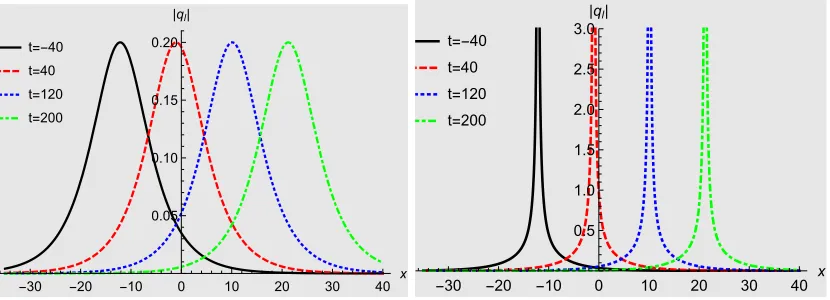
We observe that for real parameterαthe presence of the deformation parameterβ changes drastically the overall qualitative behaviour of the wave. When it is vanishing, that is in the case of the NLSE, the solution is simply a standing wave that changes its amplitude as a function of time. However, whenβis switched on the solutions of the full Hirota equation displays a qualitatively different behaviour than the one for the NLSE as the wave starts to move with a speedv=βµ2.
t=-40 t=40 t=120 t=200
-30 -20 -10 0 10 20 30 40
x
0.05 0.10 0.15 0.20
|ql|
t=-40 t=40 t=120 t=200
-30 -20 -10 0 10 20 30 40 x 0.5
1.0 1.5 2.0 2.5 3.0
[image:8.595.90.505.360.510.2]|ql|
Figure 1: Regular and singular one-soliton solutions (3.6) for the local Hirota equations (2.12) at different times forα= 0.5,β= 0.7,γ= 0.4 +i0.3, µ= 0.2 +i0.3, λ= 1forκ=−1and κ= 1in the left and right panel, respectively.
From figure 1 we also observe that for κ= 1the solution (3.6) develops a singularity. Even though these cusp solutions have possible applications [33] and are interesting in their own right, we will often just focus on the equation for κ=−1in what follows, since apart from the overall sign the actual value ofκis irrelevant as it can be absorbed into λ.
To obtain the two-soliton solution we need to go two orders further in the expansion (3.5) and use f(x, t) = 1 +ε2f2(x, t) +ε4f4(x, t), g(x, t) = εg1(x, t) +ε3g3(x, t) in the
bilinear equations (3.3), (3.4). Settingε= 1we obtain the two-soliton solution
q(2)l (x, t) = g1(x, t) +g3(x, t)
with
g1 = τµ,γ+τν,δ, (3.9)
g3 = (µ−ν) 2
(µ+µ∗)2(ν+µ∗)2τν,δ|τµ,γ|
2+ (µ−ν)2
(µ+ν∗)2(ν+ν∗)2τµ,γ|τν,δ|
2, (3.10)
f2 = |τµ,γ| 2
(µ+µ∗)2 +
τν,δτ∗µ,γ (ν+µ∗)2 +
τµ,γτ∗ν,δ (µ+ν∗)2 +
|τν,δ|2
(ν+ν∗)2, (3.11)
f4 = (µ−ν) 2(µ∗
−ν∗
)2
(µ+µ∗)2(ν+µ∗)2(µ+ν∗)2(ν+ν∗)2 |τµ,γ|
2
|τν,δ|2. (3.12)
t=-25 t=-15 t=15 t=25
-100 -50 0 50
x
0.2 0.4 0.6 0.8 1.0 1.2 1.4
|ql|
t=-25 t=-15 t=15 t=25
-60 -40 -20 0 20 40 60
x
0.2 0.4 0.6 0.8 1.0 1.2 1.4
[image:9.595.87.513.95.386.2]|ql|
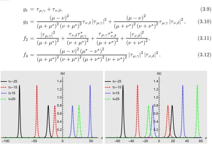
Figure 2: Modulus of the two-soliton solutions (3.8) for the local Hirota equations (2.12) at different times forα= 0.4,β= 1.8,γ= 0.3,δ= 0.4,µ= 1.3,ν = 0.8,λ= 1, κ=−1displaying a faster soliton overtaking a slower one (left panel) andγ= 0.3 +i0.1, δ= 0.4 +i0.7,µ= 1.3 +i0.5,
ν = 0.8 +i0.65,λ= 1,κ=−1displaying a head-on collision (right panel).
t=-8 t=-2 t=2 t=6
-40 -20 0 20 40 x
0.2 0.4 0.6 0.8 1.0 1.2
|ql|
t=-25 t=-15 t=15 t=25
-40 -20 0 20 40 x
0.2 0.4 0.6 0.8 1.0 1.2 1.4
|ql|
Figure 3: Modulus of the two-soliton solutions (3.8) for the local Hirota equations (2.12) at different times for α= 0.4, β = 0.8, γ = 0.3 +i0.1, δ = 0.4 +i0.7, λ = 1, κ =−1 with a left moving one-soliton withµ= 1.−i1.4, ν = 0.8 +i0.65(left panel) and a right moving one-soliton withµ= 1.3 +i0.5,ν = 0.8 +i0.65, (right panel) scattering with a static one-solition acting as a defect.
[image:9.595.88.505.467.614.2]composed of a fast one-soliton overtaking a slower one. For a complex choice of the spectral and shift parameter this behaviour is changed into a head-on collision of two one-solitons. More striking is the previously not pointed out possibility that within the two-soliton solution one of the one-solitons contributions can be made static by a suitable parameter choice. We observe in figure 3 that the static soliton can be seen as a defect. The only effect of the scattering is the usual slight displacement or time-delay depending on the reference frame.
3.2 Darboux-Crum transformations
Alternatively, the solutions of the Hirota equation can also be constructed following the Darboux-Crum transformation scheme [34, 35, 36]. At first we will keep our discussion very general by leaving the functionsq andr generic without specifying the different choices for r and consider those concrete scenarios in the next sections.
Generally speaking, Darboux transformations relate two different Hamiltonian systems by means of an intertwining relation [34, 35, 36]. The iteration of this procedure to a se-quence of Hamiltonian systems is usually referred to as the Darboux-Crum transformation scheme. In the present case we can convert one of the AKNS equations into an eigenvalue equation and thus identify a Hamiltonian of Dirac type. TakingΨto be a two-dimensional vector we obtain
Ψ = ϕ
φ , Ψx=UΨ =⇒
−iϕx+iqφ=−λϕ
iφx−irϕ=−λφ
. (3.13)
Comparing with the eigenvalue equationHΨ(λ) =−λΨ(λ), we read off the Hamiltonian
H= −i∂x iq −ir i∂x
=−iσ3∂x+V, (3.14)
from (3.13), withσ3 denoting a standard Pauli matrix. Next we seek to relate this
Hamil-tonian, together with its eigenfunctions, to a set of new Hamiltonians of similar structure
Hn= −i∂x iqn
−irn i∂x
=−iσ3∂x+Vn, (3.15)
satisfying HnΨn(λ) = −λΨn(λ) for n ∈ N. By construction the new Hamiltonians are
designed in such a way that the qn and rn satisfy the two equations resulting from the
zero curvature condition with spectral parameters λn and are therefore also solutions to
our nonlinear wave equations. Let us next discuss how to obtain them by employing the Darboux-Crum transformation scheme for Dirac Hamiltonians as discussed in [37, 38]. The key assumption is that the different Hamiltonians are recursively related to each other by intertwining relations
LnHn−1 =HnLn, (3.16)
with intertwining operatorsLn. IdentifyingH0 =H, the iteration of the equations (3.16)
Next we discuss how to obtain the intertwining operators and the potentials. We start with equation (3.16) for n= 1 and assume the intertwining operator to be of the general form L1 := I∂x+B. Upon substituting H, H1 and L1the intertwining relation yields the
two equations
V1 =V −i[B, σ3], and Vx+BV −V1B+iσ3Bx= 0. (3.17)
Taking nextB=−UxU−1, as suggested in [37], and substituting the first equation in (3.17)
into the second, the latter becomes equivalent to
U−1HU
x= 0. (3.18)
Integrating this equation leads toHU =UΛ withΛ containing the integration constants. This equation has now become formally equivalent to the Schrödinger equation with the difference that U is a matrix. Taking diag Λ = (−λ1,−λ2) this equation is solved by
U = (Ψ(λ1),Ψ(λ2)) =:U1 and thus we have found
L1 =I∂x−(U1)xU
−1
1 and V1=V +i (U1)xU
−1
1 , σ3 . (3.19)
We may now simply iterate these equations obtaining
U2= (L1Ψ(λ3), L1Ψ(λ4)), L2 =I∂x−(U2)xU
−1
2 , V2 =V1+i (U2)xU
−1 2 , σ3 ,
U3= (L2L1Ψ(λ5), L2L1Ψ(λ6)), L3 =I∂x−(U3)xU
−1
3 , V3 =V2+i (U3)xU
−1
3 , σ3 ,
..
. ... ...
Un= (LnΨ(λ2n−1),LnΨ(λ2n)), Ln=I∂x−(Un)xUn−1, Vn=Vn−1+i (Un)xUn−1, σ3 .
(3.20) What is left is to specify our original solution Ψ(λ). Adopting the notation from [38], we abbreviate Ωi = Ψ(λi) so that at level n of the iteration procedure we have a set of 2n
spinors that can be viewed as null states for the intertwining operatorLn
S2n={Ω1,Ω2, . . . ,Ω2n−1,Ω2n}, Ωi = ϕi
φi
, λi=λj, (3.21)
i.e. we haveLnΩi= 0fori= 1, ...,2n.
Having in principle computed Vn in an iterative manner, as in indicated (3.20), we
just need to read off the off-diagonal elements to identify the new solutions qn and rn,
because the Darboux-Crum scheme guarantees that they satisfy the equations (2.9) and (2.10) whenq and r are solutions. These expressions constitute the multi-soliton solutions we are seeking to construct.
To be explicit, in the first iteration step we have
L1=I∂x+ 1 detW1
detD1
1 −detD
q
1
detDr
1 detD21
, V1 =V0+ 2i
detW1
0 detD1q
detDr
1 0
, (3.22)
where we introduced the matrices
W1 = ϕ1 φ1
ϕ2 φ2
, Dq1 = ϕ
′
1 ϕ1
ϕ′
2 ϕ2
, D1r= φ
′
1 φ1
φ′
2 φ2
, D11 = ϕ
′
1 φ1
ϕ′
2 φ2
, D21 = ϕ1 φ
′
1
ϕ2 φ
′
2
.
FromV1 we read off the one-soliton solution
q1 =q+ 2ϕ
′
1ϕ2−ϕ1ϕ′2
ϕ1φ2−ϕ2φ1 , and r1 =r−2 φ′
1φ2−φ1φ
′
2
ϕ1φ2−ϕ2φ1. (3.24)
In a similar fashion we can use now (3.20) to compute iteratively the higher order solutions. Remarkably then-solition solutions can be presented in a closed compact form as
qn=q+ 2 detDqn detWn
, and rn =r−2 detDr
n detWn
, (3.25)
with Wn, Dnq and Dnr denoting 2n×2n-matrices generalizing (3.23). The determinant
of the matrix Wn corresponds to the generalized Wronskian of the set in (3.21) with n
columns containingϕi, i= 1, ...,2n, and its derivatives and ncolumns containing φi and
its derivatives with respect to x
Wn=
ϕ(1n−1) ϕ1(n−2) . . . ϕ1 φ(1n−1) . . . φ′
1 φ1
ϕ(2n−1) ϕ(2n−2) . . . ϕ2 φ (n−1) 2 . . . φ
′
2 φ2
..
. ... . .. ... ... . .. ... ... ϕ2(nn−1) ϕ2(nn−2) . . . ϕ2n φ
(n−1) 2n . . . φ
′
2n φ2n
. (3.26)
The matrix Dqn is made up of n−1 columns containingϕi and its derivatives and n+ 1
columns containingφi and its derivatives
Dnq =
φ(1n−2) φ(1n−3) . . . φ1 ϕ(
n) 1 . . . ϕ
′
1 ϕ1
φ2(n−2) φ2(n−3) . . . φ2 ϕ(2n) . . . ϕ′
2 ϕ2
..
. ... . .. ... ... . .. ... ... φ(2nn−2) φ
(n−3)
2n . . . φ2n ϕ
(n) 2n . . . ϕ
′
2n ϕ2n
, (3.27)
and the matrixDr
nis made up ofn+ 1columns containingϕi and its derivatives andn−1
columns containingφi and its derivatives
Dnr =
φ(1n) φ(1n−1) . . . φ1 ϕ(
n−2)
1 . . . ϕ
′
1 ϕ1
φ(2n) φ2(n−1) . . . φ2 ϕ(2n−2) . . . ϕ′
2 ϕ2
..
. ... . .. ... ... . .. ... ... φ2(nn) φ2(nn−1) . . . φ2n ϕ
(n−2)
2n . . . ϕ
′
2n ϕ2n
. (3.28)
Thus we obtain the2-soliton solution fromW2,Dr2 andD2r, the3-soliton solution fromW3,
Dr
3 and Dr3, etc. A closed expression for the Ln-operator can be found in [38].
Let us now construct some concrete solutions. First we need to determineΨ1by solving
(2.1). Specifying the “seed functions”q and r as r(x, t) =q(x, t) = 0, takingλ→iλ the component equations for the two linear equations (Ψ1)t=VΨ1 and (Ψ1)x =UΨ1 in (2.1)
decouple into
(ϕ1)x=λϕ1, (φ1)x =−λφ1, (ϕ1)t= 2λ2(iα−2βλ)ϕ1, (φ1)t=−2λ2(iα−2βλ)φ1.
These equations are easily solved by
Ψ1(x, t;λ) = ϕ1(x, t;λ)
φ1(x, t;λ) =
eλx+2λ2
(iα−2βλ)t+γ1
e−λx−2λ2
(iα−2βλ)t+γ2 , (3.30)
with constants γ1,γ2 ∈ C. Next we implement the constraint r(x, t) = κq∗(x, t), that
converts the local Hirota equation (2.12) into its conjugate (2.13). Given the solution (3.24) forr =q= 0this restriction leads to ϕ2 =φ
∗
1,φ2=κϕ∗1, so that
Ψ2(x, t;λ) = ϕ2(x, t;λ)
φ2(x, t;λ)
= φ
∗
1(x, t;λ)
κϕ∗
1(x, t;λ)
= e
−λ∗x+2t(λ∗)2
(iα+2βλ∗)+γ∗ 2
κeλ∗x−2t(λ∗)2
(iα+2βλ∗)+γ∗
1 . (3.31)
Substituting these expressions into (3.24) we obtain the one-soliton solution
q1(x, t) =− 2(λ+λ
∗
)e2λx+4λ2
t(iα−2βλ)+γ1−γ2
1−κe2(λ+λ∗)x+4iα(λ2
−(λ∗)2
)t−8β(λ3
+(λ∗)3
)t+γ1+γ∗1−γ2−γ∗2
. (3.32)
This solution agrees exactly with the one obtained by means of Hirota’s method in (3.6) when we set in thereλ→2(λ+λ∗
),µ→2λ,γ→γ1−γ2,κ→1. In the same way we can construct an-soliton solutions using the set
˜
S2n={Ψ1(x, t;λ1),Ψ2(x, t;λ1),Ψ1(x, t;λ2),Ψ2(x, t;λ2), ...,Ψ1(x, t;λn),Ψ2(x, t;λn)}
(3.33) with λi = λj in the evaluation of the formulae (3.25). As we shall discuss below, the
solutions to the new non-local equations are obtained by keeping the same seeds in the constructions of the wavefunctions Ψ1 and by implementing different types of constraints
in the construction of Ψ2.
We conclude with a remark on how to obtain degenerate solutions for the cases with equal eigenvalues as discussed in detail for other models in [39, 40, 41]. Instead of consid-ering the set (3.21) withΩi providedλi =λj, we need to implement Jordan states and use
the set
S2degn = Ω1,Ω2, ∂λΩ1, ∂λΩ2, . . . , ∂λn−1Ω1, ∂ n−1
λ Ω2 , Ω1 =
ϕ1
φ1 ,Ω2= ϕ2
φ2 . (3.34)
in the evaluation of the formulae (3.25). Obviously, the combinations of the two different kind of seeds are also possible giving rise to new building blocks S˜2n and S2degn .
4. The nonlocal complex parity transformed Hirota equation
In this case the compatibility between the equation (2.9) and (2.10) is achieved by the choicer(x, t) =κq∗
4.1 Hirota’s direct method
Let us now consider the new nonlocal integrable equation (2.14) forκ=−1. We factorize again q(x, t) = g(x, t)/f(x, t), but unlike as in the local case we no longer assume f(x, t)
to be real but allowg(x, t), f(x, t)∈C. We then find the identity
f3f˜∗
iqt+αqxx+ 2αq˜
∗
q2−δ(qxxx+ 6qq˜
∗
qx) = (4.1)
ff˜∗
iDtg·f +αDx2g·f −δD3xg·f + f˜
∗
Dx2f ·f−2fgg˜
∗ 3δ
f Dxg·f −αg . When comparing with the corresponding identity in the local case (3.1), we notice that this equation is of higher order in the functions involved, in this caseg,˜g∗
,f,f˜∗
, having increased from three to four. The left hand side vanishes when the nonlocal Hirota equation (2.14) holds and the right hand side vanishes when demanding
iDtg·f+αD2xg·f−δDx3g·f = 0, (4.2)
together with
˜
f∗
D2xf·f = 2fgg˜
∗
. (4.3)
We notice that equation (4.3) is still trilinear. However, it may be bilinearised by intro-ducing the auxiliary functionh(x, t)and requiring the two equations
Dx2f ·f =hg, and 2fg˜
∗
=hf˜∗
, (4.4)
to be satisfied separately. In this way we have obtained a set of three bilinear equations (4.2) and (4.4) instead of two. These equations may be solved systematically by using in addition to (3.5) the formal power series expansion
h(x, t) = kε
kh
k(x, t). (4.5)
For vanishing deformation parameterδ→0the equations (4.2) and (4.4) constitute the bi-linearisation for the nonlocal NLSE. As our equation differ from the ones recently proposed for that model in [42] we will comment below on some solutions related to that specific case. The local equations presented in the previous section are obtained forf˜∗
→f,g˜→g, h→g∗
as in this case the two equations in (4.4) combine into the one equation (3.4).
4.1.1 Two types of nonlocal one-soliton solutions
Let us now solve the bilinear equations (4.2) and (4.4). First we construct the one-soliton solutions. Unlike as in the local case we have here several options, obtaining different types. Using the truncated expansions
f = 1 +ε2f2, g=εg1, h=εh1, (4.6)
we derive from the three bilinear forms in (4.2) and (4.4) the constraining equations
0 =ε[i(g1)t+α(g1)xx−δ(g1)xxx] +ε3[2 (f2)x(g1)x−g1[(f2)xx+i(f2)t] (4.7) +if2[(g1)t+i(g1)xx]],
0 =ε2[2(f2)xx−g1h1] +ε4 2f2(f2)xx−2(f2)2x , (4.8)
0 =ε[2˜g∗
1 −h1] +ε3 2f2˜g1∗−f˜
∗
At this point we pursue two different options. At first we follow the standard Hirota procedure and assume that each coefficient for the powers in ε in (4.7)-(4.9) vanishes separately. We then easily solve the resulting six equations by
g1 =λτµ,γ, f2 = |λ| 2
(µ−µ∗)2τµ,γτ˜
∗
µ,γ, h1 = 2λ∗˜τ∗µ,γ, (4.10)
with constants γ,λ,µ∈C. Setting then ε= 1we obtain the exact one-soliton solution
qst(1) = λ(µ−µ
∗
)2τµ,γ (µ−µ∗)2+|λ|2τ
µ,γ˜τ∗µ,γ
. (4.11)
Next we only demand that the coefficient in (4.7)-(4.8) vanish separately, but deviate from the standard approach by requiring (4.9) only to hold for ε= 1. This is of course a new option that was not at our disposal for the standard local Hirota equation, since in that case the third equation did not exist. In this setting we obtain the solution
g1 = (µ+ν)τµ,iγ, f2 =τµ,iγ˜τ∗−ν,−iθ, h1= 2(µ+ν)˜τ∗−ν,−iθ, (4.12)
so that this one-soliton solution becomes
q(1)nonst = (µ+ν)τµ,iγ 1 +τµ,iγτ˜∗−ν,−iθ
. (4.13)
The standard solution (4.11) and the nonstandard solution (4.13) exhibit qualitatively different behaviour. Whereas qst(1) depends on one complex spectral and one complex shift parameter,q(1)nonst depends on two real spectral parameters and two real shift parameters. Hence the solutions can not be converted into each other. Taking in (4.11) for simplicity λ=µ−µ∗
the modulus squared of this solution becomes
qst(1) 2 = (µ−µ
∗
)2ex(µ+µ∗)
2 cosh [x(µ−µ∗)]−2 cosh γ+γ∗+it α µ2−(µ∗)2 −δ µ3−(µ∗)3 .
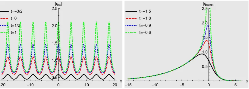
(4.14) This solution is therefore nonsingular for Reγ = 0 and asymptotically nondivergent for
Reµ = 0. We depict a regular solution in the left panel of figure 4 and observe the expected nonlocal structure in form of periodically distributed stationary breathers.
In contrast, the nonstandard solution (4.13) is unavoidably singular. We compute
qnonst(1) 2= (µ+ν)
2ex(µ−ν)
2 cosh [x(µ+ν)] + 2 cos [γ+θ+t[α(µ2−ν2)−δ(µ3+ν3)]]. (4.15)
which forx= 0becomes singular foranychoice of the parameters involved at
ts = γ+θ+ (2n−1)π
α(ν2−µ2) +δ(µ3+ν3), n∈Z. (4.16)
t=-3/2 t=0 t=1/2 t=1
-20 -10 0 10 20 x
0.5 1.0 1.5 2.0 2.5 |qst|
t=-1.5 t=-1.0 t=-0.9
t=-0.6
-15 -10 -5 0 5 x
0.5 1.0 1.5
2.0 2.5
[image:16.595.91.504.83.231.2]|qnonst|
Figure 4: Nonlocal regular one-soliton solution (4.14) for the nonlocal Hirota equations obtained from the standard Hirota method at different times for α = 0.4, δ = 0.8, γ = 0.6 +i1.3 and
µ =i0.7, λ =i1.7(left panel). Nonlocal rogue wave one-soliton solution (4.15) for the nonlocal Hirota equations obtained from the nonstandard Hirota method at different times for α = 0.4,
δ= 1.8,γ= 0.5,θ= 0.1, µ= 0.2andν= 1.2(right panel).
(4.16) that this structure is periodically repeated so that we can speak of anonlocal rogue wave [43, 44].
Notice that for α→ −1 and δ →0 the system (2.14) reduces to the nonlocal NLSE studied in [17]. For this case the solution (4.13) acquires exactly the form of equation (22) in [17] when we set ν → −2η1, µ → −2η2, γ → θ2 and θ → θ1. There is no equivalent
solution to the regular solution (4.11) reported in [17], so thatqst(1) forδ →0 is a also new solution for the nonlocal NLSE.
4.1.2 The two-parameter nonlocal two-soliton solution
As in the local case we expand our auxiliary functions two orders further in order to construct the nonlocal two-soliton solution. Using the truncated expansions
f = 1 +ε2f2+ε4f4, g=εg1+ε3g3, h=εh1+ε3h3, (4.17)
to solve the bilinear equations (4.2) and (4.4), we find
g1 =τµ,γ+τν,δ, (4.18)
g3 = (µ−ν) 2
(µ−µ∗)2(ν
−µ∗)2τµ,γτν,δ˜τ ∗
µ,γ+
(µ−ν)2 (µ−ν∗)2(ν
−ν∗)2τµ,γτν,δ˜τ ∗
ν,δ, (4.19)
f2 =
τµ,γ˜τ∗µ,γ (µ−µ∗)2 +
τν,δτ˜∗µ,γ (ν−µ∗)2 +
τµ,γ˜τ∗ν,δ (µ−ν∗)2 +
τν,δ˜τ∗ν,δ
(ν−ν∗)2, (4.20)
f4 = (µ−ν) 2(µ∗
−ν∗
)2 (µ−µ∗)2(ν
−µ∗)2(µ
−ν∗)2(ν
−ν∗)2τµ,γ˜τ ∗
µ,γτν,δ˜τ∗ν,δ, (4.21)
h1 = 2˜τ∗µ,γ+ 2˜τ
∗
ν,δ, (4.22)
h3 = 2 (µ
∗
−ν∗
)2 (µ−µ∗)2(ν∗−µ)2τ˜
∗
µ,γτ˜
∗
ν,δτµ,γ+ 2 (µ
∗
−ν∗
)2 (µ∗−ν)2(ν−ν∗)2˜τ
∗
µ,γ˜τ
∗
So that forε= 1we obtain from (4.18)-(4.23) the two-soliton solution
qnl(2)(x, t) = g1(x, t) +g3(x, t)
1 +f2(x, t) +f4(x, t). (4.24)
As for the one-soliton solution (4.11) we recover the solutions to the local equation by taking ˜τ → τ and µ∗
→ −µ∗ , ν∗
→ −ν∗
in the pre-factors. In figure 5 we depict the solution (4.24) at different times. These solutions are well localized and maintain their shape after collision, which is the reason we refer to them as nonlocal soliton solutions. Since all our solutions are nonlocal, either in space, time or both we will omit the explicit mentioning of nonlocal at times.
t=-15 t=-2 t=-1 t=10
-40 -20 0 20 40
x
1 2 3 4 5 |qn|
-40 -20 0 20 40
x
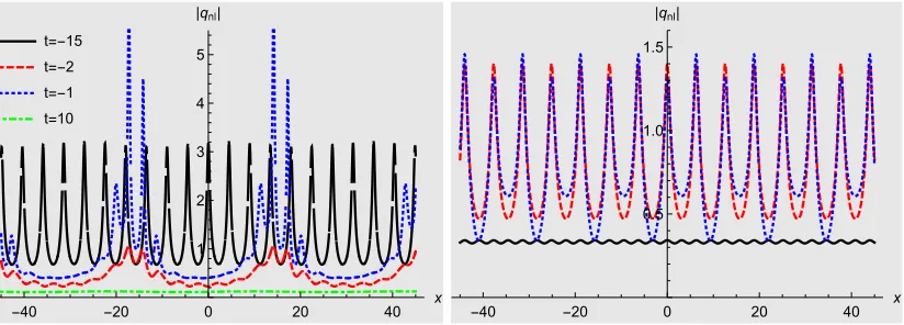
[image:17.595.92.504.242.390.2]0.5 1.0 1.5 |qnl|
Figure 5: Nonlocal regular two-soliton solution (4.24) for the nonlocal Hirota equations obtained from the standard Hirota method at different times forα= 0.4,δ= 0.8,γ1= 0.6 +i1.3,µ1=i0.7,
γ2 = 0.9 +i0.7, µ2 = i0.9 (left panel). Nonlocal regular two one-soliton solution (4.11) for the nonlocal Hirota equations γ1 = 0.6 +i1.3, µ1 = i0.7 and γ2 = 0.9 +i0.7, µ2 = i0.9 versus the nonlocal regular two-soliton solution (4.24) at the same values at timet= 2.5(right panel).
In the left panel we observe the evolution of the two-soliton solution producing a complicated nonlocal pattern. In the right panel we can see that at large time the two-soliton solutions appears to be an interference between two nonlocal one-two-solitons.
As in the construction for the one-soliton solutions we can also pursue the option to solve equation (4.9) only for ε = 1 leading to a second type of two-soliton solutions. We will not report them here, but instead discuss how they emerge when using Darboux-Crum transformations.
4.2 Darboux-Crum transformations
We start again by choosing the vanishing seed functions q = r = 0 and solve the linear equations (2.1) with λ→iλ, i.e. (3.29), with the additional constraintβ =iδ by
˜
Ψ1(x, t;λ) = ϕ1(x, t;λ)
φ1(x, t;λ)
= e
λx+2iλ2
(α−2δλ)t+γ1
e−λx−2iλ2
(α−2δλ)t+γ2 . (4.25)
In the construction of Ψ2 we implement now the constraint r(x, t) = ±q∗(−x, t), with
the previous section we expect to obtain two different types of solutions. Indeed, unlike as in the local case we have now two options at our disposal to enforce the constraint. The standard choice consists of takingϕ2=±φ˜
∗
1,φ2 = ˜ϕ∗1for complex parameters which is very
similar to the approach in local case. Alternatively we can choose hereφ1 = ˜ϕ∗
1,φ2=±ϕ˜
∗
2.
Evidently the first equation in the latter constraint holds whenγ∗
2=γ1 in (4.25). It is also
clear that the second option is not available in the local case. For the first choice we obtain therefore
˜
Ψ2(x, t;λ) = ϕ2(x, t;λ)
φ2(x, t;λ)
= ∓φ
∗
1(−x, t;λ)
ϕ∗
1(−x, t;λ)
= ∓e
λ∗x+2i(λ∗)2
(α−2δλ)t+γ∗ 2
e−λ∗x−2i(λ∗)2
(α−2δλ∗)t+γ∗
1 , (4.26)
withλ,γ1, γ2∈Cand hence for the lower sign with (3.24) we have
qst(1)(x, t) = 2(λ
∗
−λ)e2λ∗x+2i(λ∗)2
(α−2δλ∗)t−γ∗ 1+γ∗2
1 +e2(λ∗−λ)x+4i[α(λ∗)2−αλ2
+2δλ3
−2δ(λ∗)3
]t−γ1+γ2−γ∗1+γ∗2
. (4.27)
For the second choice we takeΨ1(x, t;µ) withµ∈R and γ2 =γ∗1 in (4.25). In this choice
the second wavefunction decouples entirely from the first and we may therefore also choose different parameters. Again for the lower we take
˜
Ψ2(x, t;ν) = ϕ2(x, t;ν)
φ2(x, t;ν)
= e
νx+2iν2
(α−2δν)t+γ3
−e−νx−2iν2
(α−2δν)t+γ∗
3 (4.28)
and hence (3.24) yields
q(1)nonst(x, t) =
2(ν−µ)eγ1−γ∗1+2µx+4iµ 2
(α−2δµ)t
1 +e2(µ−ν)x+4i(αµ2−αν2−2δµ3+2δν3)t+γ
1−γ∗1−γ3+γ∗3. (4.29)
The n-soliton solutions are obtained considering the set
˜
S2stn= Ψ˜1(x, t;λ1),Ψ˜2(x, t;λ1),Ψ˜1(x, t;λ2),Ψ˜2(x, t;λ2), ...,Ψ˜1(x, t;λn),Ψ˜2(x, t;λn)
(4.30) or
˜
S2nonstn = Ψ˜1(x, t;µ1),Ψ˜2(x, t;ν1),Ψ˜1(x, t;µ2),Ψ˜2(x, t;ν2), ...,Ψ˜1(x, t;µn),Ψ˜2(x, t;νn)
(4.31) with (4.25) and (4.26) and the formulae (3.25).
5. The nonlocal complex time-reversed Hirota equation
In this case the compatibility between the equations (2.9) and (2.10) is achieved by the choice r(x, t) =±q∗
scenario. Using vanishing seed functionsq=r= 0we solve the linear equations (2.1) with λ→iλ,α=iˆδ andβ =iδ by
ˆ
Ψ1(x, t;λ) = ϕ1(x, t;λ)
φ1(x, t;λ)
= e
λx−2λ2
(ˆδ+2iδλ)t+γ1
e−λx+2λ2
(ˆδ+2iδλ)t+γ2 . (5.1)
The constraintr(x, t) =±qˆ∗
(x,−t)in (3.24) can be implemented in two different ways by either takingϕ2=±φˆ
∗
1,φ2= ˆϕ
∗
1 obtaining
ˆ
Ψ2(x, t;λ) = ϕ2(x, t;λ)
φ2(x, t;λ)
= ±φ
∗
1(x,−t;λ)
ϕ∗
1(x,−t;λ)
= ±e
−λ∗x−2(λ∗)2
(ˆδ−2iδλ∗)t+γ∗ 2
eλ∗x+2(λ∗)2
(ˆδ−2iδλ∗)t+γ∗ 1
, (5.2)
orφ1= ˆϕ∗
1,φ2 =±ϕˆ
∗
2 with λ=µ∈iR,γ2 =γ
∗
1 and new constantsν ∈iR,γ2 ∈Cso that
we have
ˆ
Ψ2(x, t;ν) = ±ϕ2(x, t;ν)
φ2(x, t;ν) =
±eνx−2ν2
(ˆδ+2iδν)t+γ2
e−νx+2ν2
(ˆδ+2iδν)t+γ∗
2 . (5.3)
The corresponding one-soliton solutions computed with (3.24) are therefore
qst(1)(x, t) = ±2(λ+λ
∗
)e2λx+γ1+γ∗2
e2x(λ+λ∗)+4(λ∗)2(ˆδ−2iδλ∗)t+γ
1+γ∗1∓e4λ 2
(ˆδ+2iδλ)t+γ2+γ∗2
, (5.4)
and
qnonst(1) (x, t) = ±2(µ−ν)e
2x(µ+ν)+γ1+γ2
e2µx+4ν2(ˆδ+2iδν)t+γ
1+γ∗2 ∓e2νx+4µ
2(ˆδ+2iδµ)t+γ 2+γ∗1
. (5.5)
The nonlocality is now only felt in time for fixed values of x, but we expect to find well localized solutions in space for fixed values of t. It is clear how to compute then-soliton solutions, simply by using the set
ˆ
S2stn= Ψˆ1(x, t;λ1),Ψˆ2(x, t;λ1),Ψˆ1(x, t;λ2),Ψˆ2(x, t;λ2), ...,Ψˆ1(x, t;λn),Ψˆ2(x, t;λn)
(5.6) or
ˆ
S2nonstn = Ψˆ1(x, t;µ1),Ψˆ2(x, t;ν1),Ψˆ1(x, t;µ2),Ψˆ2(x, t;ν2), ...,Ψˆ1(x, t;µn),Ψˆ2(x, t;νn)
(5.7) with (5.1) and (5.2) and the formulae (3.25).
An interesting special case is obtained for ˆδ = 0, which correspond to a complex nonlocal time-reverse version of the modified KdV equation. In this case the solution (5.4) has no poles for the lower sign and is asymptotically finite fort→ ±∞as long asReγ1= 0
and Reγ2 = 0. We depict some one and two-soliton solutions for the case in figure 6. We observe from the local nature of the solutions in space and the feature that the two-soliton solution has one-soliton constituents. As shown in figure 6 when shifting the parameters in the one-soliton solutions appropriately they match exactly the one-soliton constituents in the two-soliton solution. However, this only happens at special instances in time and the solutions will not keep oscillating in synchronicity when time evolves, even for large values of time.
|q(2)|, t=-100 |q(1)|,Δ
1=2
|q(1)|,Δ
=0
-10 -5 0 5 10x
02 0 0 0 1.0 12 1
|qst|
|q(2)|, t=1507.8 |q(1)|,Δ1=1.54 |q(1)|,Δ1=-0.68
-10 -5 0 5 10x
0.2 0.4 0.6 0.8 1.0 1.2 1.4 |qst|
|q(2)|, t=500.37 |q(1)|,Δ1=0
|q(1)|,Δ
2=-2.73
-10 -5 0 5 10x
1 2 3 4 5 6
[image:20.595.83.509.84.183.2]|qst|
Figure 6: Modulus of two one-soliton solutions (5.4) and the corresponding two-soliton solutions for the complex nonlocal time-reverse version of the modified KdV equation atˆδ= 0,δ= 1.0and different values of time. The one-solitons are computed at forλ = 0.3, γ1 = 0.3 + ∆1 γ2 = 0.2 and λ = 0.4, γ1 = 0.2 + ∆2 γ2 = 0.5. The two-soliton is computed for the same values with
∆1= ∆2= 0.
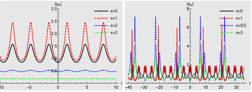
x=0 x=1 x=
x= 3
-10 -5 0 5 10
t 0.5 1.0 1.5 3 |qst|
=0 =1 =5/ =
-4 - - -10 0 10
t
4 6 8 |qst|
Figure 7: Time crystal structures in the complex nonlocal time-reverse version of the modified KdV equation atˆδ= 0, δ= 1.0and different points in space. The one-soliton solutions (5.4) are computed forλ= 0.5, γ1 = 0.2andγ2= 0.8(left panel). The two-soliton solutions are computed at forλ1= 0.6, γ1= 0.2,γ2= 0.8, λ2= 0.3,γ3= 0.2andγ4= 0.5(right panel).
6. The nonlocal complex PT-transformed Hirota equation
In this case the compatibility between the equation (2.9) and (2.10) is achieved by the choice r(x, t) =±q∗
(−x,−t) when taking κ=±1. As x and t are now directly related to
−x and −t, we expect some nonlocality to emerge in space as well as in time. With seed functionsq =r = 0,α=iˇδ,ˇδ, β ∈Rwe solve the linear equations (2.1) by
ˇ
Ψ1(x, t;λ) = ϕ1(x, t;λ)
φ1(x, t;λ) =
eλx−2λ2
(ˇδ+2βλ)t+γ1
e−λx+2λ2
(ˇδ+2βλ)t+γ2 . (6.1)
Implementing the constraint r(x, t) = ±q∗
(−x,−t) in (3.24) by ϕ2 = ±φˇ
∗
1, φ2 = ˇϕ∗1 we
obtain
ˇ
Ψ2(x, t;λ) = ϕ2(x, t;λ)
φ2(x, t;λ)
= ∓φ
∗
1(−x,−t;λ)
ϕ∗
1(−x,−t;λ)
= ∓e
−λ∗x−2(λ∗)2
(ˇδ+2βλ∗)t+γ∗ 2
eλ∗x+2(λ∗)2(ˇδ+2βλ∗)t+γ∗1 ,
[image:20.595.94.505.267.417.2]orφ1= ˇϕ∗
1,φ2 =−ϕˇ
∗
2 withλ=µ∈R,γ2=γ
∗
1 and new constantsν∈R, γ2 ∈Cwe have
ˇ
Ψ2(x, t;ν) = −ϕ2(x, t;ν)
φ2(x, t;ν)
= −e
νx−2ν2
(ˇδ+2βν)t+γ2
e−νx+2ν2
(ˇδ+2βν)t+γ∗
2 . (6.3)
The corresponding one-soliton solutions computed with (3.24) are therefore
qst(1)(x, t) = ±2(λ−λ
∗
)eγ1+γ∗2+2(λ+λ∗)x
eγ1+γ∗1+4(λ∗)
2(2βλ∗+ˇδ)t+2µx
±eγ2+γ∗2+4λµ
2(2βλ+ˇδ)t+2λ∗x, (6.4)
and
qnonst(1) (x, t) = 2(ν−µ)e
γ1−γ∗1+2(µ+ν)x
e4µ2
(2βµ+ˇδ)t+2νx+e4ν2
(2βν+ˇδ)t+2µx. (6.5)
With (6.1) and (6.2) in the sets
ˇ
Sst2n= ˇΨ1(x, t;λ1),Ψˇ2(x, t;λ1),Ψˇ1(x, t;λ2),Ψˇ2(x, t;λ2), ...,Ψˇ1(x, t;λn),Ψˇ2(x, t;λn)
(6.6) or
ˇ
S2nonstn = ˇΨ1(x, t;µ1),Ψˇ2(x, t;ν1),Ψˇ1(x, t;µ2),Ψˇ2(x, t;ν2), ...,Ψˇ1(x, t;µn),Ψˇ2(x, t;νn)
(6.7) then-soliton solutions are computed from the formulae (3.25).
As discussed above, the choicesr(x, t) =±q(−x, t) and r(x, t) =±q(x,−t) with real qs are less interesting and will therefore not discuss the here.
7. The nonlocal conjugate PT-transformed Hirota equation
In this case the compatibility between the equation (2.9) and (2.10) is achieved by the choice r(x, t) =κq(−x,−t) withκ∈C. As in the previous section we takeq =r = 0, but
with no further restrictions on the parameters involved and solve the linear equations (2.1) to
ˇ
Ψ1(x, t;λ) = ϕ1(x, t;λ)
φ1(x, t;λ) =
eλx+2λ2
(iα−2βλ)t+γ1
e−λx−2λ2
(iα−2βλ)t+γ2 . (7.1)
When implementing the constraintr(x, t) =κq(−x,−t)in (3.24) by ϕ2 =κˇφ∗1,φ2= ˇϕ∗
1 we
obtain a Ψ2(x, t;λ) leading todetD1q= detDr1= 0so that the standard solution does not
exist in this case. However, implementing φ1 =i√κϕˇ1, by taking eγ2 = i√κeγ1, λ→ µ
and likewise for φ2 = −i√κϕˇ2 with new spectral parameters λ→ν and shift parameter γ3 =γ1 we obtain
qnonst(1) (x, t) = 2i(µ−ν)e
2µx+4iµ2
(α+2iβµ)t
√
κ 1 +e2x(µ−ν)+[4iα(µ2−ν2
)+8β(ν3−µ3
)]t . (7.2)
which means thatqnonst(1) (x+∆1, t+∆2)with∆1,∆2∈Cis also a solution that will, however,
in general not satisfy the constraintr(x, t) =κq(−x,−t). Note that this operation does not constitute a full variable substitution, i.e. the differentials are not replaced. Then-soliton solutions are obtained by using the set
ˇ
Snonst2n = ˇΨ1(x, t;µ1),Ψˇ2(x, t;ν1),Ψˇ1(x, t;µ2),Ψˇ2(x, t;ν2), ...,Ψˇ1(x, t;µn),Ψˇ2(x, t;νn) ,
(7.3) in the formulae (3.25).
8. Conserved charges
Since our models are integrable we may employ standard techniques to compute all con-served charges. Following [47] and references therein we define two new complex valued fieldsT(x, t)and χ(x, t) in terms of the components of the auxiliary fieldΨintroduced in (2.1). The local conservation law in terms of these fields
T := ϕx
ϕ, χ:=− ϕt
ϕ, ⇒ Tt+χx = 0 (8.1)
is trivially satisfied. The two first rows in the second equation in (2.1) then yield
T =qφ
ϕ−iλ, χ=−A−B φ
ϕ, (8.2)
so that the local conservation law in (8.1) becomes
Tt− A+iλB+ B
qT x = 0. (8.3)
DifferentiatingT in (8.1) with respect to xthe Ricatti equation
Tx =iλqx
q +rq−λ
2+qx
q T−T
2, (8.4)
which needs to be solved for the at this stage unknown functionT that also solves (8.3). An infinite number of charges be obtained from the Gardner transformation [48, 49, 50, 40] that is defined by expandingT in terms ofλand a new fieldwintroduced asT =−iλ[1−
w/(2λ2)]. Substituting this Ansatz for T into the Ricatti equation (8.4) with a further convenient parametrisationλ=i/(2ε) leads to the relation
w+ε wx− qx
q w +ε
2w2
−rq= 0. (8.5)
At this stage our discussion describes the two equations (2.9) and (2.10) for the two in-dependent functionsr(x, t) and q(x, t). Expanding the new auxiliary density fields w(x, t)
as
w(x, t) =
∞
n=0
we can obtain the functionswn order by order in εin a recursive recursive manner.
Sub-stituting the expansion for w(x, t)into (8.5) yields the recurrence relation
wn= qx
q wn−1−(wn−1)x−
n−2
k=0
wkwn−k−2, forn≥1. (8.7)
Taking from (8.5)w0 =rq, the first expressions are calculated to
w1 = −qrx, (8.8)
w2 = −q2r2+qrxx, (8.9)
w3 = qr2qx+ 4q2rrx−qrxxx, (8.10)
w4 = 2q3r3−6qrqxrx−5q2rx2−qr2qxx−6q2rrxx+qrxxxx (8.11)
Given the local conservation law, it follows that the quantities In =
∞
−∞wndx are all conserved in time for all choices of the functionsr as described in section 2.
9. Conclusions
We exploited various possibilities involving different combinations of parity, time-reversal and complex conjugation to achieve compatibility between the two equations (2.9) and (2.10) resulting from the zero curvature condition for the Hirota equation. Each possibility corresponds to a new type of integrable system. Solving these new nonlocal equations by means of Hirota’s direct method we encountered various new features. Instead of having to solve two bilinear equations, these new systems correspond to three bilinear equations involving an auxiliary function. We solved these equations in the standard fashion by using a formal expansion parameter that in the end can be set to any value when the expansions are truncated at specific orders. In addition, the new auxiliary equation allows for a new option for this equation to be solve for a specific value of the expansion parameter, thus leading to a new type of solution different from the one obtained in the standard fashion. We also identified the mechanism leading to this second type of solution within the approach of using Darboux-Crum transformations. In that context the nonlocal relations betweenq and r allow for different options in (3.24).
We have found various different type of behaviours. For the local Hirota equation the sign of the parameter κdetermines whether the solutions are regular or singular whereas tuning the spectral parameter can produce two soliton solutions with a faster one overtaking a slower one, a head-on collision and, most interestingly, a solution in which one of the solitons behaves like a defect. The nonlocal complex parity transformed Hirota equation has two different types of solutions displaying a nonlocal structure of periodically distributed stationary breathers or rogue waves. The nonlocal complex time-reversed Hirota equation possesses regular localized solutions in space, but is nonlocal in time displaying some time crystal like structures.
also left aside the study of further interesting properties, such as degeneracies, time-delays etc., which were considered in [51, 39, 40, 41]. As the approach we followed is general, further new models related to integrable or even nonintegerable realizations of HNLSE (1.1) other than the Hirota equation can be constructed and possibly different types of systems altogether. The most interesting challenge is to investigate whether these nonlocal solutions can be realized experimentally. Delocalized states occur for instance in optical beam propagation in nonlinear dielectric waveguides with random varied refractive index, spacing or size [52]. Furthermore, in [53] it was shown that the nonlocal NLSE is gauge equivalent to an unconventional model of coupled Landau-Lifshitz equations that describes the physics of nanomagnetic artificial materials. Finally, it would also be interesting to perform the inverse scattering transform for the nonlocal Hirota system along the lines of [54], where it was carried out for the nonlocal nonlinear Schrödinger equation. The soliton solutions we constructed here, via the Darboux-Crum transformations, are based on coupled eigenfunctions which display a particular symmetry at x → ±∞, see section 4.2. This suggest the procedure in [54], could also applied be applied for the system treated here when adopting some extra symmetry conditions.
Acknowledgments: JC is supported by a City, University of London Research Fellowship. FC was partially supported by Fondecyt grant 1171475. AF would like to thank the Instituto de Ciencias Físicas y Matemática at the Universidad Austral de Chile for kind hospitality and financial support.
References
[1] A. Shabat and V. Zakharov, Exact theory of two-dimensional self-focusing and
one-dimensional self-modulation of waves in nonlinear media, Sov. Phys. JETP34(1), 62—69 (1972).
[2] G. P. Agrawal, Fiber-optic communication systems, volume 222, John Wiley & Sons, 2012.
[3] P. K. Shukla and B. Eliasson, Nonlinear aspects of quantum plasma physics, Physics-Uspekhi 53(1), 51—76 (2010).
[4] L. F. Mollenauer, R. H. Stolen, and J. P. Gordon, Experimental observation of picosecond pulse narrowing and solitons in optical fibers, Phys. Rev. Lett.45(13), 1095 (1980).
[5] F. M. Mitschke and L. F. Mollenauer, Discovery of the soliton self-frequency shift, Optics Letters11(10), 659—661 (1986).
[6] J. P. Gordon, Theory of the soliton self-frequency shift, Optics letters 11(10), 662—664 (1986).
[7] Y. Kodama and A. Hasegawa, Nonlinear pulse propagation in a monomode dielectric guide, IEEE Journal of Quantum Electronics23(5), 510—524 (1987).
[8] D. Anderson and M. Lisak, Nonlinear asymmetric self-phase modulation and self-steepening of pulses in long optical waveguides, Phys. Rev. A27(3), 1393 (1983).
[10] M. Wadati and K. Sogo, Gauge transformations in soliton theory, J. Phys. Soc. Japan52(2), 394—398 (1983).
[11] N. Sasa and J. Satsuma, New-type of soliton solutions for a higher-order nonlinear Schrödinger equation, J. Phys. Soc. Japan60(2), 409—417 (1991).
[12] R. Hirota, Exact envelope-soliton solutions of a nonlinear wave equation, J. Math. Phys.
14(7), 805—809 (1973).
[13] A. Fring, PT-symmetric deformations of integrable models, Phil. Trans. Royal Soc. London A: Math., Phys. and Eng. Sci. 371(1989), 20120046 (2013).
[14] F. K. Abdullaev, Y. V. Kartashov, V. V. Konotop, and D. A. Zezyulin, Solitons in PT-symmetric nonlinear lattices, Phys. Rev. A83(4), 041805 (2011).
[15] N. V. Alexeeva, I. Barashenkov, A. A. Sukhorukov, and Y. S. Kivshar, Optical solitons in PT-symmetric nonlinear couplers with gain and loss, Phys. Rev. A85(6), 063837 (2012).
[16] V. V. Konotop, J. Yang, and D. A. Zezyulin, Nonlinear waves in PT-symmetric systems, Rev. of Mod. Phys.88(3), 035002 (2016).
[17] M. J. Ablowitz and Z. H. Musslimani, Integrable nonlocal nonlinear Schrödinger equation, Phys. Rev. Lett. 110(6), 064105 (2013).
[18] M. J. Ablowitz and Z. H. Musslimani, Integrable nonlocal nonlinear equations, Studies in Applied Mathematics (2016).
[19] A. Khare and A. Saxena, Periodic and hyperbolic soliton solutions of a number of nonlocal nonlinear equations, J. of Math. Phys.56(3), 032104 (2015).
[20] M. Li and T. Xu, Dark and antidark soliton interactions in the nonlocal nonlinear Schrödinger equation with the self-induced parity-time-symmetric potential, Phys. Rev. E
91(3), 033202 (2015).
[21] A. S. Fokas, Integrable multidimensional versions of the nonlocal nonlinear Schrödinger equation, Nonlinearity29(2), 319 (2016).
[22] S. V. Suchkov, A. A. Sukhorukov, J. Huang, S. V. Dmitriev, C. Lee, and Y. S. Kivshar, Nonlinear switching and solitons in PT-symmetric photonic systems, Laser & Photonics Reviews10(2), 177—213 (2016).
[23] T. Valchev, On Mikhailov’s reduction group, Phys. Lett. A379(34), 1877—1880 (2015).
[24] V. Caudrelier, Interplay between the Inverse Scattering Method and Fokas’s Unified Transform with an Application, arXiv:1704.05306, Studies in Applied Mathematics (2017).
[25] M. Gürses and A. Pekcan, Nonlocal Nonlinear Schr\" odinger Equations and Their Soliton Solutions, arXiv preprint arXiv:1707.07610 (2017).
[26] J. Weiss, M. Tabor, and G. Carnevale, The Painlevé property for partial differential equations, J. Math. Phys.24, 522—526 (1983).
[27] J. Weiss, The Painlevé property for partial differential equations. II: Bäcklund
transformation, Lax pairs, and the Schwarzian derivative, J. Math. Phys. 24, 1405—1413 (1983).
[29] M. J. Ablowitz, D. J. Kaup, A. C. Newell, and H. Segur, Nonlinear-evolution equations of physical significance, Phys. Rev. Lett.31(2), 125 (1973).
[30] R. Hirota, The direct method in soliton theory, volume 155, Cambridge University Press, 2004.
[31] W.-J. Liu, B. Tian, H.-Q. Zhang, L.-L. Li, and Y.-. Xue, Soliton interaction in the higher-order nonlinear Schrödinger equation investigated with Hirota’s bilinear method, Phys. Rev. E77(6), 066605 (2008).
[32] J. Hietarinta, A search for bilinear equations passing Hirota’s three-soliton condition. IV. Complex bilinear equations, J. Math. Phys.29(3), 628—635 (1988).
[33] J. Eggers, Air entrainment through free-surface cusps, Phys. Rev. Lett.86(19), 4290(4) (2001).
[34] G. Darboux, On a proposition relative to linear equations, physics/9908003, Comptes Rendus Acad. Sci. Paris94, 1456—59 (1882).
[35] M. M. Crum, Associated Sturm-Liouville systems, The Quarterly Journal of Mathematics
6(1), 121—127 (1955).
[36] V. B. Matveev and M. A. Salle, Darboux transformation and solitons, (Springer, Berlin) (1991).
[37] L. M. Nieto, A. A. Pecheritsin, and B. F. Samsonov, Intertwining technique for the one-dimensional stationary Dirac equation, Annals. of Phys.305(2), 151—189 (2003).
[38] F. Correa and V. Jakubsk`y, Confluent Crum-Darboux transformations in Dirac Hamiltonians with PT-symmetric Bragg gratings, Phys. Rev. A 95(3), 033807 (2017).
[39] F. Correa and A. Fring, Regularized degenerate multi-solitons, Journal of High Energy Physics2016(9), 8 (2016).
[40] J. Cen, F. Correa, and A. Fring, Time-delay and reality conditions for complex solitons, J. of Math. Phys.58(3), 032901 (2017).
[41] J. Cen, F. Correa, and A. Fring, Degenerate multi-solitons in the sine-Gordon equation, J. Phys. A: Math. Theor.50, 435201 (2017).
[42] S. Stalin, M. Senthilvelan, and M. Lakshmanan, Nonstandard bilinearization of PT-invariant nonlocal nonlinear Schrödinger equation: Bright soliton solutions, Phys. Lett. A381(30), 2380—2385 (2017).
[43] C. Kharif and E. Pelinovsky, Physical mechanisms of the rogue wave phenomenon, Euro. J. of Mech.-B/Fluids22(6), 603—634 (2003).
[44] A. Chabchoub, N. P. Hoffmann, and N. Akhmediev, Rogue wave observation in a water wave tank, Phys. Rev. Lett.106(20), 204502 (2011).
[45] F. Wilczek, Quantum time crystals, Phys. Rev. Lett.109(16), 160401 (2012).
[46] A. Shapere and F. Wilczek, Classical time crystals, Phys. Rev. Lett.109(16), 160402 (2012).
[47] J. Cen and A. Fring, Asymptotic and scattering behaviour for degenerate multi-solitons in the Hirota equation, Physica D: Nonlinear Phenomena 397, 17—24 (2019).
[49] R. M. Miura, The Korteweg-de Vries Equation: A Survey of Results, SIAM Review18, 412—459 (1976).
[50] B. A. Kupershmidt, On the nature of the Gardner transformation, Journal of Mathematical Physics22(3), 449—451 (1981).
[51] J. Cen and A. Fring, Complex solitons with real energies, J. Phys. A: Math. Theor.49(36), 365202 (2016).
[52] T. Pertsch, U. Peschel, J. Kobelke, K. Schuster, H. Bartelt, S. Nolte, A. Tünnermann, and F. Lederer, Nonlinearity and disorder in fiber arrays, Phys. Rev. Lett. 93(5), 053901 (2004).
[53] T. A. Gadzhimuradov and A. M. Agalarov, Towards a gauge-equivalent magnetic structure of the nonlocal nonlinear Schrödinger equation, Phys. Rev. A 93(6), 062124 (2016).