https://doi.org/10.1007/s00500-019-04154-5
M E T H O D O L O G I E S A N D A P P L I C A T I O N
Adaptive multi-population inflationary differential evolution
Marilena Di Carlo1 ·Massimiliano Vasile1·Edmondo Minisci1
© The Author(s) 2019
Abstract
This paper proposes a multi-population adaptive version of inflationary differential evolution algorithm. Inflationary dif-ferential evolution algorithm (IDEA) combines basic difdif-ferential evolution (DE) with some of the restart and local search mechanisms of Monotonic Basin Hopping (MBH). In the adaptive version presented in this paper, the DE parametersCRand
Fare automatically adapted together with the size of the local restart bubble and the number of local restarts of MBH. The proposed algorithm implements a simple but effective mechanism to avoid multiple detections of the same local minima. The novel mechanism allows the algorithm to decide whether to start or not a local search. The algorithm has been extensively tested over more than fifty test functions from the competitions of the Congress on Evolutionary Computation (CEC), CEC 2005, CEC 2011 and CEC 2014, and compared against all the algorithms participating in those competitions. For each test function, the paper reports best, worst, median, mean and standard deviation values of the best minimum found by the algo-rithm. Comparisons with other algorithms participating in the CEC competitions are presented in terms of relative ranking, Wilcoxon tests and success rates. For completeness, the paper presents also the single population adaptive IDEA, that can adapt onlyCRandF, and shows that this simpler version can outperform the multi-population one if the radius of the restart bubble and the number of restarts are properly chosen.
Keywords Global optimisation·Differential evolution·Multi-population algorithm·Adaptive algorithm
1 Introduction
Differential evolution (DE), proposed by Price et al. (2006), is a well-known population-based evolutionary algorithm for solving global optimisation problems over continuous spaces. Literature indicates that DE exhibits very good per-formance over a wide variety of optimisation problems (Das and Suganthan2011). However, although being a very efficient optimiser, its local search ability has long been questioned and work has been done to improve its local
con-Communicated by V. Loia.
B
Marilena Di CarloMassimiliano Vasile
Edmondo Minisci
1 Department of Mechanical and Aerospace Engineering,
James Weir Building, 75 Montrose Street, Glasgow G1 1XJ, UK
vergence by combining DE with local optimisation strategies (Qing2010).
In previous works by the authors, Locatelli and Vasile (2015) and Vasile et al. (2011), it was demonstrated that DE can converge to a fixed point, a level set or a hyperplane that does not contain the global minimum. The collapse of the population to a fixed point or a neighbourhood of a fixed point from which DE cannot escape was one of the motiva-tion for the development of inflamotiva-tionary differential evolumotiva-tion algorithm (Vasile et al.2011).
during the search process can be found in the literature, (Brest et al.2006, 2013; Liu and Lampinen2005; Omran et al.2005); a parameter-less adaptive evolutionary algorithm has been presented in Papa (2013). However, no approach has been proposed so far to adaptδlocal andnLR. In this paper, we present a simple mechanism to adapt CR and
F within a single population and a multi-population strat-egy to adaptδlocal and nLR. The multi-population version of IDEA is in the following called MP-AIDEA (Multi Pop-ulation Adaptive Inflationary Differential Evolution Algo-rithm).
The resulting algorithm was extensively tested over 51 test problems from the single objective global optimisation competitions of the Congress on Evolutionary Computation (CEC) 2005, 2011 and 2014. Tests to assess the performance of the algorithm include rankings, Wilcoxon test and suc-cess rate. It will be shown that the adaptive version of IDEA always ranks in the first three best algorithms in every com-petition for every number of dimensions except for the CEC 2014 test set with 30 dimensions. Furthermore, it will be shown that the simple adaptation ofCRandF within a sin-gle population can outperform the multi-population version with adaptation ofδlocalandnLRif these two parameters are properly chosen.
This paper extends the work presented in Di Carlo et al. (2015). In Di Carlo et al. (2015), the basic mechanisms that constitute MP-AIDEA were introduced, and the per-formance of MP-AIDEA was measured only by a relative ranking against other algorithms. This paper provides a more detailed explanation of all the mechanisms and heuristics inside MP-AIDEA; moreover, it presents an extensive empir-ical assessment of its performance, using several metrics in addition to the relative ranking. As part of this extensive performance evaluation, we compare MP-AIDEA against a number of other algorithms and a single population version of MP-AIDEA with no adaptive local restart. Detailed results obtained for each test functions are also presented, so that the paper can be used as a reference for comparison against other algorithms.
The paper starts stating the problem we are trying to solve in Sect.2and briefly introducing the basic principles and fun-damental theoretical developments underneath inflationary differential evolution in Sect.3. The adaptation mechanisms are presented, together with the resulting adaptive multi-population version of IDEA, MP-AIDEA, in Sect. 5. The test cases are presented in Sect.6, and the obtained results are presented in Sect.6.1. Finally, the paper presents the results of all the comparative tests in Sects.6.2,6.3and6.4. Section7concludes the paper.
2 Problem statement
This paper is concerned with the following class of global minimisation problems with box constraints:
min
x∈B f(x) (1)
with f :B ⊆RnD →R,n
Dthe number of dimensions and the boxBdefined by the upper and lower boundariesxlower≤ x ≤ xupper. In the following, we will use a gradient-based local search algorithm; therefore, we further require that f ∈ C2(B). Note, however, that this is not a strict requirement as we can show that the algorithm can work also when a finite number of non-differentiable points exist.
3 Inflationary differential evolution
This section briefly recalls the working principles of infla-tionary differential evolution and presents the parameters that the algorithm proposed in this paper adapts. Following the notation introduced in Vasile et al. (2011), we express the general DE process as a discrete dynamical system. The gov-erning equation, for the i-th individual at generation k, is expressed as:
xi,k+1=xi,k+S(xi,k+ui,k,xi,k)ui,k (2) with
ui,k =e
Gxr1,k+(1−G)xi,k+F(xr2,k−xr3,k)
+ (1−G)F(xbest,k−xi,k)
(3)
where G can be either 0 or 1 [with G = 1 corresponding to the DE strategy DE/rand andG = 0 corresponding to the DE strategy DE/current-to-best (Price et al.2006)]. In Eq. (3),r1,r2andr3are integer numbers randomly chosen in the population, andeis a mask containing random numbers of 0 and 1 according to:
et =
1⇒U≤C R
ut,i,k=
xt,i,k+xt,lower
/2, ifut,i,k <xt,lower
xt,i,k+xt,upper
/2, ifut,i,k >xt,upper
(5)
The selection functionSis defined as:
S(xi,k+ui,k,xi,k)=
1 if f(x
i,k+ui,k) < f(xi,k)
0 otherwise (6)
In the general case in which the indicesr1,r2andr3can assume any value, in Vasile et al. (2011) it was demonstrated that the population can converge to a fixed point different from a local minimum or to a level set. Furthermore, in Locatelli and Vasile (2015) it was demonstrated that DE can converge to a hyperplane that does not contain the global minimum. Finally, consider the following proposition.
Proposition 1 Consider the subsetΨ = {x∈B: f(x)≤ ¯f} and the supersetφsuch that:
1. Ψ ⊂φ 2. xi,k+1∈φ,∀i
3. ∀y∈φ\Ψ ,f(y) > f¯
then if the population at iteration k is entirely contained in Ψ it cannot escape fromΨ at any future iteration.
Proof The proof descends from the definition of S. Sup-pose that a candidate individualxi,k+1was generated by map (2) then, because of point 3 of the proposition, it would be rejected by the selection operator.
Therefore, when the population contracts within a ballBc⊆
Ψ of radiusρl, DE can only converge to a point or a subset withinBc. We callρlthe contraction limit, in the following. In inflationary differential evolution, the DE heuristics is iterated until the population reaches the contraction limit. A local search is then started from the best individual in the pop-ulationxbest, the corresponding local minimumxLMis saved in an archive of local minimaAand the population is restarted in a bubbleBRof radiusδlocalaround the local minimumxLM. This mechanisms is borrowed from the basic logic under-neath monotonic basin hopping (Wales and Doye1997). To assess if the contraction condition is satisfied, the maximum distance between all possible combinations of individuals of the population at generationk,ρ(k), is computed:
ρ(k)=max||x
i,k−xl,k||
i,l=1, . . . ,Npop (7) where Npop is the number of individuals in the popula-tion. The contraction is verified whenρ(k) ≤ ¯ρρmax, where
ρmax=maxkρ(k)is the maximum value ofρever recorded until generationkandρ¯is one of the parameters of the algo-rithm, the contraction threshold. This contraction criterion
is consistent with Proposition1 under the assumption that
ρl = ¯ρρmax.
After a number nLR of such local restarts, without any improvement of the current best solution, the archiveA col-lects all the local minima found so far. At this point, the population is restarted globally in the search space so that every individual is initially at a distance√nDδglobalfrom the centres of the clusters of the local minima inA. During local restarts, the most important information is preserved in the local minimum. The assumption is that the basin of attrac-tion of that local minimum has already been explored and that exploration led to the convergence of the population to
Bc. When the population is restarted globally the essential information, all the local minima, is stored in the archiveA. Here the assumption is that IDEA has completely explored a funnel structure resulting in a cluster of minima.
These restart procedures were proven to be very effective in a series of difficult real problems in which the landscape presents multiple funnels (see Vasile et al.2011for additional details).
The complete inflationary differential evolution process with trial vector (3) is governed by the following key param-eters: Npop, CR and F, G, ρ¯, δlocal, nLR, δglobal. From experience, we know thatδglobalis not a critical parameter in most of the cases whileCR,F,δlocalandnLRplay a signif-icant role and are not always easy to define. The parameters
CRandF are applied to update each individual in a popu-lation whileδlocal andnLR are applied to restart the whole population. Therefore, in this paper we propose two adapta-tion mechanisms, one for CRandF and one for δlocal and
nLR. In particular, the adaptation mechanisms ofCR,Fand
δlocalare such as to result in the definition of numerical val-ues for these parameters, to be used by the algorithm. On the contrary, the use ofnLRis replaced by a mechanism that allows the algorithm to decide when to perform a local or global restart, so that the definition of a numerical value for
nLRis not required anymore.
4 Adaptation mechanisms
Because of the very nature ofCRandF,δlocalandnLR, the automatic adaptation ofCRandF requires only the evalua-tion of the success of each candidate incrementui,k. On the other hand, the adaptation ofδlocalandnLRrequires the eval-uation of the success of the restart of an entire population. Therefore, in this paper it is proposed to extend the working principle of inflationary differential evolution by evolving
over a set of possible values ofCRandF, that evolves with the population.
All populations are then concurrently adaptingδlocaland the number of local restarts. More specifically, the adaptation mechanism of the local restart bubble evolves a probabil-ity distribution function over a range of possible values of
δlocal. Each population draws values from that probability distribution and at each local restart increases the probabil-ity associated to the value ofδlocal that led to a transition from one local minimum to another. The range ofδlocal is also adapted by taking the mean and the minimum distance among the local minima inA.
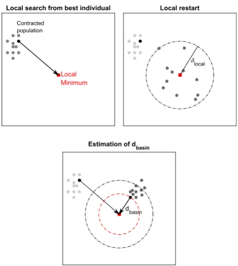
The number of local restarts, instead, is dictated by the contraction of a population within the basin of attraction of an already identified local minimum. Given a local minimum xLM ∈ Aand a list ofnbest,L M best individuals from which a local search converged to xLM, the size of the basin of attraction ofxLMis defined as
dbasin,L M =min
j ||xbest,j−xLM||, j ∈1, ...,nbest,L M (8) Each local minimumxLM in A, therefore, is associated to a particulardbasin,L M. Figure1 illustrates this mechanism. Oncedbasin,L M is estimated, every time the conditionρm(k)≤
¯
ρρm,maxis satisfied for populationm, if the best individual xbest,m is at a distance lower thandbasin,L M fromxLM, then no local restart is performed but the population is restarted globally in the search space. The numbernbest,L M is set to 4 in this implementation.
The overall algorithm, called Multi-Population Adap-tive Inflationary Differential Evolutionary Algorithm (MP-AIDEA), is described in more detail in the following section.
5 Multi-population adaptive inflationary
differential evolution
MP-AIDEA is described in Algorithm1. Let npop be the number of populations andmthe index identifying each pop-ulation. With reference to Algorithm1, after initialisation of main parameters and functionalities (Algorithm1, line1), MP-AIDEA starts by runningnpop Differential Evolutions in parallel, one per population (Algorithm1, line3). Dur-ing each evolution process, the parameters F and CRare automatically adapted following the approach presented in Sect.5.2. When a populationmcontracts within a ballBcof radiusρ ρ¯ m,max, the evolution of that population is stopped. Once all the populations have contracted, the relative posi-tion of the best individual of each populaposi-tion,xbest,m with respect to the local minima in A,xLM, is assessed (Algo-rithm1, line7). This step makes use of all the minima found by all populations and, therefore, it has to be regarded as an
Local Minimum Local search from best individual
Contracted population
δlocal
Local restart
dbasin Estimation of dbasin
Fig. 1 Identification of the basin of attraction of local minimumxLM
Algorithm 1MP-AIDEA
1: Initialisation (Section5.1, Algorithm2) 2:form∈ [1, . . . ,npop]do
3: Run Differential Evolution with adaptiveC RandFuntil con-traction toBc(Section5.2, Algorithms3and4)
4:end for
5:form∈ [1, . . . ,npop]do
6: xbest,m=ar gmi nxm,i∈Pmf(xm,i)
7: if(∀L M : [xbest,m−xL M>dbasi n,L M oriL M<nbest,L M]) orA= ∅then
8: Run local search and find local minimumx(sm)
mi n,m 9: sm=sm+1
10: if∃L M : x(sm)
mi n,m−xL M ≤εΔthen 11: iL M=iL M+1
12: dbasi n,L M=min[dbasi n,L M,||xbest,m−xL M||]
13: L Rm=1
14: else
15: xL M←x(mi nsm),m
16: Store local minima xL M in A, compute dbasi n,L M = xbest,m−xL M
17: L Rm=1
18: end if 19: else 20: L Rm=0 21: end if 22:end for
23: Update distribution ofδlocal(Algorithm6)
24: Restart populations with Algorithm7usingL Rm,δlocalandδglobal
25: If total number of function evaluations is lower than maximum number of function evaluations,nf eval,max, goto (2)
[image:4.595.307.543.52.316.2]attraction of any previously detected local minimum (that is, ∀L M : xbest,m−xLM>dbasin,L M) then a local search is run (Algorithm1, line8) and the resulting local minimum is stored in the archive A(Algorithm1, line16). The flag for the local restart,L Rm, is set to 1. On the contrary, if the best individual of populationmis inside the basin of attraction of a previously detected local minimum, the local search is not performed andL Rmis set to 0 (Algorithm1, line20).
Before running a local or a global restart (Algorithm1, line24), the probability distribution associated toδlocaland its range are updated (Algorithm1, line23). After restarting the population, if the number of maximum function evaluations,
nfeval,max, is not exceeded, the process restarts from line2in Algorithm1. Each part of Algorithm1is explained in more details hereafter.
5.1 Initialisation
The steps for the initialisation of MP-AIDEA are presented in Algorithm2. MP-AIDEA starts with the initialisation ofnpop populations, withNpopindividuals each, in the search space
B. The number of function evaluations for each population is set to zero,nfeval,m =0 andρ¯,δglobal, are initialised to the values specified by the user. The counter of the number of local search per population,sm, is set to 0.
Algorithm 2MP-AIDEA: initialisation
1: Set values fornpop,Npop,ρ¯,δglobal,ε,sm=0∀m∈ [1, . . . ,npop]
2: Setnfeval,m=0 andkm=1 (generation number) for each popula-tionsm∈ [1, . . . ,npop]
3: Initialize populationPmwith individualsxm,i∀m ∈ [1, . . . ,npop] and∀i∈ [1, . . . ,Npop]
4: ComputeΔ= xupper−xlowerwherexlower andxupper are the lower and upper boundaries of the search space
5.2 Differential evolution and the adaptation of
CR
and
F
For each populationm, a DE process is run (Algorithm 3, line6), using Equations2,3,4and6. The parameterG, in Equation3, assumes values equal to 0 or 1 with probabil-ity 0.5. During the advancement from parents to offspring, each individual of the population is associated to a differ-ent value ofCRandF, drawn from a distributionCRF(km)
m (Algorithm 3, lines 1, 2, 3). CRF(km=1)
m is initialised as a uniform distribution with(nD+1)2 points in the space
CR∈ [0.1,0.99]andF∈ [−0.5,1](Algorithm3, line1). A Gaussian kernel is then allocated to each node and a proba-bility density function is built by Parzen approach (Minisci and Vasile2014). The values ofCRandF to be associated to the individuals of the population are drawn from this
dis-tribution (Algorithm3, line4). A change valueddlinked to each kernel is initialised to zero (Algorithm3, line3) and is used during the advancement of the population from parents to children to adapt CRand F (Algorithm 3, line 8). The adaptation ofCRandF is summarised in Algorithm4and described in the following.
Algorithm 3Differential Evolution with adaptiveC RandF
1: Regular meshesCRandFwith(nD+1)2points (nDis the dimen-sionality of the problem) in the spaceC R ∈ [0.1,0.99] ×F ∈
[−0.5,1]are created 2: InitializeCRF(km=1)
m with points of the mesh:CRF(mk,mq=,11)←CRq
andCRF(km=1)
m,q,2 ←Fqfor allq∈ [1, . . . , (nD+1)2] 3: Associate to each row ofCRF(km=1)
m an elementddm(k,mq=1)=0 for allq∈ [1, . . . , (nD+1)2]
4: SampleCR(km)
m andF(mkm)from a bi-variate distribution on the two dimensional lattice defined by the rows ofCRF(km=1)
m 5:fori∈ [1, . . . ,Npop]do
6: x(km+1)
m,i ←DE x( km)
m,i ,CR( km)
m ,F(mkm)
7: nf eval,m=nf eval,m+1 8: UpdateCRF(km)
m (Algorithm4) 9:end for
10:km=km+1 11: Row sortCRF(km+1)
m in terms ofddm(km+1)values 12: Computeρ(km)
m =max(||x(mkm,i)−x( km)
m,l ||)∀x( km)
m,i ,x( km)
m,l ∈P( km)
m
13: Untilρ(km)
m ≤ ¯ρ·ρm,max, whereρm,max =max
ρ(km=1)
m , ρm(km=2), . . . ρm(km)
, orkm <10D, goto (4)
Algorithm 4Updating the joint distributionCRF
1:if f(x(km+1)
m,i ) < f(x( km)
m,i )then 2: Compute d f(km+1)
m,i = ||f(x( km+1)
m,i ) − f(x( km)
m,i)|| ∀i ∈ [1, . . . ,npop]
3: forq∈ [1, . . . , (nD+1)2]do
4: ifddm,q< d fm(k,mi+1)then 5: CRF(km)
m,q,2←F(
km)
m,i 6: dd(km)
m,q ←d fm(k,mi+1) 7: ifd f(km+1)
m,i > C RCthen
8: CRF(km)
m,q,1←C R(
km)
m,i 9: end if
10: end if 11: end for 12:end if
For each individuali of each populationm, the adapta-tion mechanism forCRandFis started only if the child is characterised by an objective function value lower than the parent’s one, that is f(x(km+1)
m,i ) < f(x
(km)
m,i )(Algorithm4, line1). If this condition is verified, the difference in objective function between parent and child at subsequent generation,
d f(km+1)
m,i = ||f(x
(km+1) m,i )− f(x
(km)
(Algo-rithm4, line2). Then the sorted elements ofCRF(km)
m are
sequentially evaluated; theq-th value ofCRinCRF(km)
m is
identified asCRF(km)
m,q,1and theq-th value of Fis identified asCRF(km)
m,q,2. The first time thatdd( km)
m,q (thedd value asso-ciated to theq-th row ofCRF(km)
m ) is lower than d fm(k,mi+1) (Algorithm4, line4), the differential weightF(km)
m,i used for the individualx(km)
m,i substitutesCRF( km)
m,q,2andd f( km+1) m,i sub-stitutesdd(km)
m,q (Algorithm4, lines5and6). This is because
F(km)
m,i produced a bigger decrease in the objective function thanCRF(km)
m,q,2(as shown byd f( km+1) m,i >dd(
km)
m,q). ForCR, the value associated tox(km)
m,i substitutes CRF( km)
m,q,1 (Algo-rithm4, line8) only ifd f(km+1)
m,i is greater than a given value
C RC(Algorithm4, line7), (Minisci and Vasile2014). The DE stops according to the contraction condition pre-sented in Sect.3. In order to prevent an excessive use of resources when the population partitions, a fail safe crite-rion was introduced that stops the DE after 10Dgenerations (Algorithm3, line13).
5.3 Local search and restart mechanisms
After the evolution of all populations has stopped, MP-AIDEA checks if the best individual of each population is inside the basin of attraction of any previously detected local minimum (see Algorithm1, line7). If that is not the case, a local search is performed from the best individual and the population is locally restarted within a hypercube with edge equal to 2δlocalaround the detected local minimum; other-wise, no local search is performed and the population is restarted globally in the whole search space (Algorithm1, line24). Prior to the implementation of the restart mecha-nisms, MP-AIDEA updates the estimation of the size of the basin of attraction of each minimum, the archiveA(see Algo-rithm1, lines5to22) and the distribution over the possible values of 2δlocal(see Algorithm1, line23). In the following the identification of the basin of attraction, the estimation of
δlocaland the two restart mechanisms are described in more details.
5.3.1 Identification of the basin of attraction
In order to mitigate the possibility of running multiple local searches that converge to already discovered local minima, MP-AIDEA estimates for each local minimum inAthe radius of the basin of attraction of that local minimum. The radius of the basin of attraction is here defined as the distancedbasin,L M from a given local minimumxLMsuch that if the best individ-ual in populationm,xbest,m, is at a distance fromxLMlower thandbasin,L Ma local search starting fromxbest,mwould con-verge toxLM.
The radiusdbasin,L M is estimated with the simple proce-dure in Algorithm1, lines7 to19. Once the evolution of all populations has stopped, the distancexbest,m−xLMof the best individual, in each population, with respect to all the minima in Ais calculated and compared to thedbasin,L M associated to each local minimum inA; initially alldbasin,L M are set to 0. If the distancexbest,m −xLMis grater than
dbasin,L Ma local search is started fromxbest,m. If the resulting local minimumx(sm)
min,malready belongs toA, the counteriLM is updated and the new estimate of the basin of attraction of xLMbecomesdbasin,L M =min[dbasin,L M,xbest,m−xLM]. x(sm)
min,m belongs to Aif∃ L M : x( sm)
min,m −xLM ≤εΔ.ε is set to 10−3. IfiLMexceeds a given maximum value and
xbest,m−xLM <dbasin,L M ∀ L Mno local search and no local restart are performed. The counteriLMis initialised to 1 for every new local minimum and keeps track of the number of times a local minimum is discovered.
5.3.2 Adaptation ofılocal
When a populationmis locally restarted, individuals are gen-erated by taking a random sample, with Latin Hypercube, within a hypercube with edge equal to 2δlocal,m. The dimen-sion δlocal,m is drawn from a probability distribution that is progressively updated at every restart. We use a kernel approach with kernels centred in the elements of a vector B(see Algorithm 6) containing a range of possible values of δlocal,m. The vectorBis initialised, with the procedure presented in Algorithm 5, when all populations performed a local search for the first time and at every global restart. During initialisation the distance between all the local min-ima in the archive Ais computed (Algorithm5, line1) and Bis initialised with values spanning the interval between the minimum and the mean distance among minima (Algorithm 5, lines 2–3). The mean values instead of the max is used to limit the size of the restart bubble and speed up conver-gence under the assumption that a local restart needs to lead to the local exploration of the search space. In the experi-mental tests, it will be shown that this working assumption is generally verified andδlocal,m tends to converge to small values. Then, a second vectorddb, with the same number of components ofB, is initialised to zero (Algorithm5, line4). During the update phase ofδlocal,m, MP-AIDEA uses the index sm to keep track of the number of times population
m performed a local search and calculates the difference
pm between two subsequent local minima (see Algorithm6, line 5). The value pm is then compared to the elements in ddband whenddb,q <pmthenδlocal,mreplacesBq, andpm replacesddb,q(Algorithm6, lines7-10). In other words, if the
δlocal,mused to restart populationmled to a local minimum x(sm)
identified by the same population, the probability of sampling
δlocal,m is increased.
Algorithm 5InitialiseB 1: Computedmi n M I N anddmi n M E AN
2: Create 1-dimensional regular grid with(nD+1)points in the interval [dmi n M I N,dmi n M E AN]
3: InitialiseBwith points of the grid
4: Initialise vectorddbassociated toBwith elementddb,q=0 for all
q∈ [1, . . . , (nD+1)]
Algorithm 6Update the distribution ofδlocal 1:ifAll populations did local search for the 1st timethen 2: Create vectorBusing Algorithm5
3:end if
4:form∈ [1, . . . ,npop]do
5: Computepm= ||x(mi nsm),m−xmi n(sm−,m1)|| 6: forq∈ [1, . . . ,nD+1]do 7: if ddb,q< pmthen 8: Bq←δlocal,m 9: ddb,q←pm 10: end if 11: end for 12:end for
13: Row sortBaccording toddbvalues
Algorithm 7MP-AIDEA: local and global restart
1:form∈ [1, . . . ,npop]do 2: ifL Rm=1then
3: Sampleδlocal,mfrom the kernel distribution over the values in B
4: L.R.: Initialise population Pm in a hypercube centred in x(sm)
mi n,mwith edge 2δlocal,mfor allm∈ {1, . . . ,npop} 5: else
6: Cluster local minima inAand compute cluster baricentresxc 7: G.R.: Initialise population√ Pm = {xm,i : ||xm,i −xc|| >
nDδglobal,∀i∈ {1, . . . ,Npop}} 8: Initialise vectorBusing Algorithm5
9: end if 10:end for
5.3.3 Local and global restart
After the identification of the basin of attraction and the update of the value ofδlocal, populations undergo a restart process in which a new population is generated either by sampling a neighbourhood of a local minimum (local restart) or by sampling the whole search space (global restart). The two restart procedures are described in Algorithm7.
The local restart procedure takes the latest identified local minimumx(sm)
min,mof populationmand restart the population
with Latin Hypercube sampling in a box centred inx(sm) min,m with edge length 2δlocal,m.
The global restart procedure identifies clusters of local minima with a Fuzzy C-Mean algorithm (Bezdek 1981), computes the centre of each cluster and initialises population
m so that each individual is at distance at least√nDδglobal from each of the centres of the clusters (Algorithm7, lines6 and7).
At each local and global restart, the CRFmatrix is re-initialised while the vectorBis initialised only after every global restart. The motivation for re-initialisingCRFat every restart is twofold: on the one hand different values ofCRand
F might be optimal in different parts of the search space, and on the other hand convergence to the optimal value of
CRand F is not always guaranteed. In search spaces with uniform and homogeneous structures, restartingCRFandB might lead to an overhead on the computational cost; there-fore, in future implementations we will test the possibility of retainingCRFandBacross the restart process.
5.4 Computational complexity
The computational complexity of MP-AIDEA is defined by the three main sets of operations:
– Local search. The local search uses the Matlabfmincon
function which implements an SQP scheme with BFGS estimation of the Hessian matrix. Since the matrix is gen-erally dense, its decomposition isO(n3D).
– Adaptation of CR and F. The adaptation ofCRandF
for each individual in each population is the other expen-sive bit of the algorithm and isO(npopNpopn2D)( see line2 in Algorithm1, line8in Algorithm3and line 3in Algo-rithm4). As a comparison, the computational complexity of the standard DE isONpop
.
– Restart mechanisms.The cost of the local restart proce-dure is limited to the generation ofnpopNpopindividuals, while the global restart has a cost associated also to clus-tering, which isO=(n2LMnDniter)(Bezdek1981), where
niteris the number of iterations for the clustering, and one associated to the verification that the new population is far from the clusters, which isO(NpopnLM)(see line7 of Algorithm7).
Overall whennpopNpop<nDthe dominant algorithmic cost is the local search while the adaptation ofCRandFbecomes more expensive for large and numerous populations. Since in the experimental test cases we will use Npop = nD and
Table 1 Functions of the CEC
2005 test set Unimodal functions
1 Shifted sphere function
2 Shifted Schwefel’s problem
3 Shifted rotated high conditioned elliptic function 5 Schwefel’s problem with global optimum on bounds Multimodal functions
6 Shifted Rosenbrock’s function
7 Shifted rotated Griewank’s function without bounds
8 Shifted rotated Ackley’s function with global optimum on bounds
9 Shifted Rastrigin’s function
10 Shifted rotated Rastrigin’s function 11 Shifted rotated Weierstrass function
12 Schwefel’s problem
13 Expanded extended Griewank’s plus Rosenbrock function
14 Shifted rotated expanded Scaffer’s
Hybrid composition functions
15 Hybrid composition function
16 Rotated hybrid composition function
18 Rotated hybrid composition function
19 Rotated hybrid composition function with narrow basin for the global opt. 20 Rotated hybrid composition function with the global optimum on the bounds
21 Rotated hybrid composition function
22 Rotated hybrid composition function with high condition number matrix
Table 2 Functions of the CEC
2011 test set 1 Parameter estimation for frequency-modulated sound waves (nD=6)
2 Lennard-Jones potential problem (nD=30)
3 The bifunctional catalyst blend optimal control problem (nD=1)
5 Tersoff potential for model Si(B) (nD=30)
6 Tersoff potential for model Si(C) (nD=30)
7 Spread spectrum radar polyphase code design (D=20)
10 Circular antenna array design problem (nD=12)
12 Messenger: spacecraft trajectory optimisation problem (nD=26)
13 Cassini 2: spacecraft trajectory optimisation problem (nD=22)
6 Experimental performance analysis
The effectiveness of MP-AIDEA is tested on a benchmark composed of three test sets. The three test sets are made of functions taken from three past competitions of the Congress on Evolutionary Computation (CEC). We took 20 functions from CEC 2005 (Suganthan et al.2005), 9 real-world prob-lems from CEC 2011 (Das and Suganthan 2010) and 22 functions from CEC 2014 (Liang et al. 2013), for a total of 51 different problems. The list of functions used in each test set is reported in Tables1,2and3. They include both aca-demic test functions and real-world optimisation problems. Since we are interested in solving problem (1), all functions selected for this benchmark are continuous and differentiable
We used four different metrics to evaluate MP-AIDEA against the algorithms that participated in the three CEC com-petitions:
– Metric 1: Best, worst, median, mean and standard devia-tion of the best result over a given number of independent runs of the algorithm.
– Metric 2: Ranking against the other algorithms using the same ranking approach proposed in the CEC 2011 com-petition.
Table 3 Functions of the CEC
2014 test set Unimodal functions
1 Rotated high conditioned elliptic function
2 Rotated Bent Cigar function
3 Rotated Discus function
Multimodal functions
4 Shifted and rotated Rosenbrock’s function
5 Shifted and rotated Ackley’s function
7 Shifted and rotated Griewank’s function
8 Shifted Rastrigin’s function
9 Shifted and rotated Rastrigin’s function
10 Shifted Schwefel’s function
11 Shifted and rotated Schwefel’s function
13 Shifted and rotated HappyCat function
14 Shfited and rotated HGBat function
15 Shifted and rotated expanded Griewank’s plus Rosenbrock’s function 16 Shfited and rotated expanded Scaffer’s F6 function
Hybrid function
17 Hybrid function 1
18 Hybrid function 2
20 Hybrid function 4
21 Hybrid function 5
Composition function
23 Composition function 1
24 Composition function 2
25 Composition function 3
28 Composition function 6
Table 4 Settings for the CEC 2005, CEC 2011 and CEC 2014 test
functions
CEC 2005 CEC 2011 CEC 2014
Problems settings
nD 10, 30, 50 – 10, 30, 50, 100
nfeval,max 10000 nD 150000 10000 nD
nruns 25 25 51
MP-AIDEA settings
npop 4 4 4
Npop nD nD nD
¯
ρ 0.2 0.2 0.2
δglobal 0.1 0.1 0.1
– Metric 4: Success rate. This is used to compare MP-AIDEA to the algorithm participating in the CEC 2011 and CEC 2014 for which the source code is available online.
The settings of MP-AIDEA were maintained constant for all problems within a particular test set and were changed going from one test set to another. This is in line with the
way all the other algorithms competed. Table4summarises the parameters and settings used for the CEC 2005, CEC 2011 and CEC 2014 test functions. More details about the chosen parameters will be given in Sect.6.1.
The ranking of the algorithms participating in every com-petition was adjusted to account only for their performance on the selected subset of differentiable functions.
It will be shown that all metrics lead to similar conclu-sions: MP-AIDEA ranks among the first four algorithms, if not first, in all three test sets and for all dimensions. We will also show that MP-AIDEA can detect previously undiscov-ered minima on some particularly difficult functions.
The current implementation of MP-AIDEA can be found open source at https://github.com/strath-ace/smart-o2c together with the benchmark of test cases.
6.1 Test sets
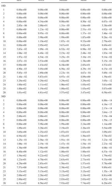
Table 5 Objective functions error of the CEC 2005 test set in dimension 10D and 30D
Best Worst Median Mean Std
10D
1 0.00e+00 0.00e+00 0.00e+00 0.00e+00 0.00e+00
2 0.00e+00 1.14e−13 0.00e+00 0.00e+00 4.34e−14
3 0.00e+00 0.00e+00 0.00e+00 0.00e+00 0.00e+00
5 5.60e−06 1.70e−04 6.17e−05 6.59e−05 4.36e−05
6 3.04e−10 2.33e−09 1.80e−09 1.60e−09 6.06e−10
7 4.83e−13 1.48e−02 1.02e−10 1.97e−03 4.21e−03
8 2.00e+01 2.00e+01 2.00e+01 2.00e+01 6.65e−10
9 0.00e+00 9.95e−01 0.00e+00 3.98e−02 1.99e−01
10 0.00e+00 3.98e+00 1.99e+00 1.79e+00 1.04e+00
11 3.29e+00 5.88e+00 5.31e+00 4.71e+00 6.18e−01
12 0.00e+00 1.19e−12 5.68e−14 1.71e−13 2.79e−13
13 9.87e−03 5.31e−01 2.66e−01 2.40e−01 1.58e−01
14 3.32e−01 3.52e+00 2.13e+00 2.11e+00 6.70e−01
15 0.00e+00 4.00e+02 2.84e−14 2.98e+01 8.14e+01
16 0.00e+00 1.15e+02 1.00e+02 9.53e+01 2.25e+01
18 3.00e+02 9.00e+02 8.00e+02 7.18e+02 2.43e+02
19 3.00e+02 9.06e+02 8.00e+02 7.45e+02 2.03e+02
20 3.00e+02 9.38e+02 8.00e+02 6.83e+02 2.46e+02
21 3.00e+02 8.00e+02 3.00e+02 4.20e+02 1.50e+02
22 3.00e+02 8.01e+02 7.54e+02 6.53e+02 2.01e+02
30D
1 0.00e+00 0.00e+00 0.00e+00 0.00e+00 0.00e+00
2 0.00e+00 2.27e−13 1.14e−13 5.68e−14 6.46e−14
3 0.00e+00 0.00e+00 0.00e+00 0.00e+00 0.00e+00
5 1.81e−01 1.52e+00 4.58e−01 5.13e−01 2.97e−01
6 5.81e−10 4.07e+00 8.25e−03 3.45e−01 8.95e−01
7 4.26e−13 1.79e−11 2.64e−12 4.58e−12 4.86e−12
8 2.00e+01 2.00e+01 2.00e+01 2.00e+01 9.26e−13
9 0.00e+00 5.97e+00 2.21e+00 2.40e+00 1.49e+00
10 1.99e+01 4.78e+01 3.18e+01 3.05e+01 7.16e+00
11 1.57e+01 2.69e+01 2.09e+01 2.12e+01 2.99e+00
12 8.24e−12 5.89e+02 1.05e+01 1.22e+02 2.06e+02
13 8.88e−01 2.66e+00 1.64e+00 1.60e+00 4.44e−01
14 1.10e+01 1.26e+01 1.17e+01 1.17e+01 3.77e−01
15 2.27e+01 4.00e+02 4.00e+02 3.15e+02 1.37e+02
16 4.16e+01 6.85e+01 5.68e+01 5.69e+01 6.99e+00
18 8.00e+02 9.11e+02 9.09e+02 8.87e+02 4.43e+01
19 8.00e+02 9.12e+02 9.06e+02 8.73e+02 5.14e+01
20 8.00e+02 9.13e+02 9.07e+02 8.78e+02 4.99e+01
21 5.00e+02 5.00e+02 5.00e+02 5.00e+02 4.91e−11
22 8.78e+02 9.22e+02 9.10e+02 9.06e+02 1.04e+01
6.1.1 CEC 2005 test set
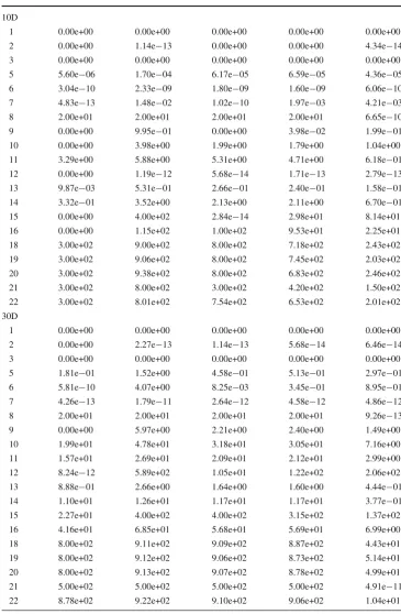
Following the rules of the CEC 2005 competition, MP-AIDEA was applied to the solution of the problems in the CEC 2005 test set in dimension nD = 10, 30 and 50,
with a maximum number of function evaluation equal to
Table 6 Objective functions error of the CEC 2005 test set in dimension 50D
Best Worst Median Mean Std
1 0.00e+00 0.00e+00 0.00e+00 0.00e+00 0.00e+00 2 5.68e−14 5.68e−13 1.14e−13 5.68e−14 1.45e−13 3 0.00e+00 0.00e+00 0.00e+00 0.00e+00 0.00e+00 5 8.28e−01 1.97e+01 2.52e+00 4.25e+00 4.82e+00 6 3.80e−10 3.11e+01 2.58e+01 2.27e+01 8.82e+00 7 6.11e−12 2.25e−07 8.05e−11 1.00e−08 4.50e−08 8 2.00e+01 2.00e+01 2.00e+01 2.00e+01 2.00e−12 9 4.97e+00 1.29e+01 7.96e+00 8.41e+00 2.14e+00 10 5.47e+01 1.01e+02 7.66e+01 7.61e+01 1.17e+01 11 3.62e+01 5.94e+01 4.57e+01 4.64e+01 6.50e+00 12 4.80e+01 9.37e+03 8.07e+02 1.24e+03 1.84e+03 13 2.87e+00 5.00e+00 3.96e+00 3.89e+00 6.35e−01 14 2.04e+01 2.19e+01 2.12e+01 2.12e+01 4.13e−01 15 2.57e+01 4.00e+02 2.88e+02 3.08e+02 1.00e+02 16 5.10e+01 7.65e+01 6.08e+01 6.25e+01 6.96e+00 18 3.04e+02 9.34e+02 9.24e+02 8.65e+02 1.30e+02 19 8.00e+02 9.34e+02 9.25e+02 8.92e+02 5.85e+01 20 3.00e+02 9.65e+02 9.13e+02 8.52e+02 1.32e+02 21 5.00e+02 5.00e+02 5.00e+02 5.00e+02 7.65e−08 22 9.20e+02 9.70e+02 9.48e+02 9.50e+02 1.31e+01
2005 competition were not included in the test set because non-differentiable.
The number of populations in MP-AIDEA was set to
npop = 4 and the number of individuals in each popula-tion was set toNpop = nD. The number of populations to
be deployed on a particular problem depends on the type and complexity of that problem, and the available number of function evaluations. We tested MP-AIDEA with dif-ferent numbers of populations from 1 to 4 (results using MP-AIDEA with one population are presented in Sect.6.2). Results showed that MP-AIDEA with 4 populations performs consistently well on all benchmarks, and, thus, we decided to present our findings fornpop =4. The contraction limit was set toρ¯ =0.2 and the global restart distance was set to
δglobal=0.1 (Table4). In line with the metrics presented at the CEC 2005 competition, Tables5and6reports the differ-ence, in the objective value, between the result obtained with MP-AIDEA and the known global minimum.
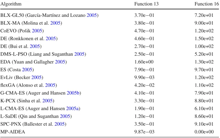
Table 7 reports the best objective function error values obtained by all the algorithms participating in the CEC 2005 competition and MP-AIDEA for functions 13 and 16 and
nD = 10. According to the CEC 2005 specifications, the accuracy level for the detection of the global minimum is 10−2for these functions. MP-AIDEA is able to identify the global minimum of both functions 13 and 16. Previously only EvLib (Becker2005) succeeded in identifying the global minimum of function 13 and no other algorithm managed to find the global minimum of function 16.
6.1.2 CEC 2011 test set
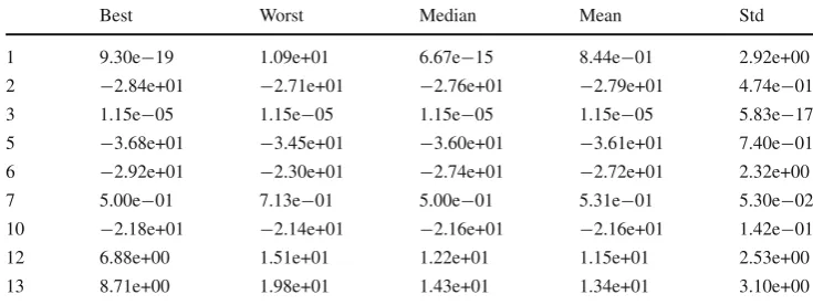
[image:11.595.178.546.482.712.2]Following the rules of the CEC 2011 competition (Das and Suganthan2010), MP-AIDEA was run fornfeval,max = 150000 function evaluations on the CEC2011 test set. The experiments were repeated fornruns=25 independent runs. Test functions with equality and inequality constraints were not included in the tests. The number of populationsnpop
Table 7 CEC 2005 best
objective function error values for functions 13 and 16, nD=10
Algorithm Function 13 Function 16
BLX-GL50 (García-Martínez and Lozano2005) 3.70e−01 7.20e+01
BLX-MA (Molina et al.2005) 3.80e−01 9.00e+01
CoEVO (Pošik2005) 4.70e−01 1.20e+02
DE (Ronkkonen et al.2005) 4.60e−01 1.50e+02
DE (Bui et al.2005) 2.70e−01 1.00e+02
DMS-L-PSO (Liang and Suganthan2005) 2.50e−01 5.20e+01
EDA (Yuan and Gallagher2005) 1.60e+00 1.30e+02
ES (Costa2005) 7.90e−01 9.70e+01
EvLiv (Becker2005) 9.90e−03 1.20e+02
flexGA (Alonso et al.2005) 4.20e−02 1.10e+02
G-CMA-ES (Auger and Hansen2005b) 4.10e−01 7.90e+01
K-PCX (Sinha et al.2005) 3.30e−01 8.80e+01
L-CMA-ES (Auger and Hansen2005a) 1.90e−01 6.10e+01
L-SaDE (Qin and Suganthan2005) 1.20e−01 8.60e+01
SPC-PNX (Ballester et al.2005) 3.50e−01 9.10e+01
Table 8 Objective functions of
the CEC 2011 test set Best Worst Median Mean Std
1 9.30e−19 1.09e+01 6.67e−15 8.44e−01 2.92e+00
2 −2.84e+01 −2.71e+01 −2.76e+01 −2.79e+01 4.74e−01
3 1.15e−05 1.15e−05 1.15e−05 1.15e−05 5.83e−17
5 −3.68e+01 −3.45e+01 −3.60e+01 −3.61e+01 7.40e−01
6 −2.92e+01 −2.30e+01 −2.74e+01 −2.72e+01 2.32e+00
7 5.00e−01 7.13e−01 5.00e−01 5.31e−01 5.30e−02
10 −2.18e+01 −2.14e+01 −2.16e+01 −2.16e+01 1.42e−01
12 6.88e+00 1.51e+01 1.22e+01 1.15e+01 2.53e+00
13 8.71e+00 1.98e+01 1.43e+01 1.34e+01 3.10e+00
was set to 4 and the number of individuals in each population was set toNpop=30 regardless of the dimensionality of the problem. The contraction limit and the global restart distance were set, respectively, toρ¯ =0.2 andδglobal =0.1 (Table
4). Table8reports the best, worst, median, mean objective function found by MP-AIDEA and the associated standard deviation.
6.1.3 CEC 2014 test set
In line with the rules of the CEC 2014 competition (Liang et al.2013), MP-AIDEA was applied to the solution of the functions in the CEC 2014 test set in dimensionnD=10, 30, 50 and 100, with maximum number of function evaluations
nfeval,max = 10000nD. The experiments were repeated for
nruns=51 independent runs. Non-differentiable functions 6, 12, 19, 22, 26, 27, 29 and 30 were not included in the test set (see Table3). The number of populations was set tonpop=4 and the number of individuals in each population was set toNpop = nD. The contraction limit and the global restart distance were set, respectively, toρ¯=0.2 andδglobal =0.1 (Table4).
Tables9and10report the difference between the objective value found by MP-AIDEA and the known global minimum. In agreement to the guidelines of the competition error values smaller than 10−8are reported as zero, (Liang et al.2013). Table11reports the best objective function values obtained by all the algorithms participating in the competition and MP-AIDEA for functions 9, 10, 11 and 15 in 10 dimensions. MP-AIDEA finds the global minimum of function 11, unlike all the other competing algorithms, and gives good results for the other functions.
6.2 Ranking
In this section, MP-AIDEA is ranked against a group of algo-rithms participating in each CEC competition. The rankings include those algorithms that reported their results in a paper and MP-AIDEA with two different settings:
– npop=4 andNpop=nD. This settings will be indicated as “MP-AIDEA” in the following and corresponds to the settings that was used to generate the results in Sect.6.1. – npop =1, Npop = 4nD; MP-AIDEA adaptsCRand F but uses fixed values for δlocal andnLR. In particular,
nLR = 10 andδlocal = 0.1, unless otherwise specified. This settings will be indicated as “MP-AIDEA,npop = 1” in the following.
The ranking method follows the rules of the CEC 2011 com-petition, (Suganthan2011). All algorithms are ranked on the basis of the best and mean values of the objective function obtained over a certain number of runs. The following pro-cedure is used to obtain the ranking:
– for each function, algorithms are ranked according to the best objective value;
– for each function, algorithms are ranked according to the mean objective value;
– the ranking for the best and mean objective values of a particular algorithm are added up over all the problems to get the absolute ranking.
In the following, the rankings obtained for the CEC 2005, CEC 2011 and CEC 2014 test sets are presented.
6.2.1 CEC 2005 test set
Table 9 Objective functions error of the CEC 2014 test set in dimension 10D and 30D
Best Worst Median Mean Std
10D
1 0.00e+00 0.00e+00 0.00e+00 0.00e+00 0.00e+00
2 0.00e+00 0.00e+00 0.00e+00 0.00e+00 0.00e+00
3 0.00e+00 0.00e+00 0.00e+00 0.00e+00 0.00e+00
4 0.00e+00 4.34e+00 0.00e+00 8.50e−02 6.07e−01
5 2.85e−06 2.00e+01 1.31e−05 1.84e+00 5.38e+00
7 0.00e+00 1.23e−02 0.00e+00 2.51e−03 4.02e−03
8 0.00e+00 9.95e−01 0.00e+00 1.37e−01 3.46e−01
9 0.00e+00 3.98e+00 1.99e+00 1.87e+00 9.26e−01
10 0.00e+00 1.19e+02 1.87e−01 9.33e+00 2.79e+01
11 0.00e+00 2.95e+02 3.67e+01 8.82e+01 8.69e+01
13 3.83e−02 1.09e−01 6.52e−02 6.98e−02 1.69e−02
14 1.06e−02 6.40e−02 2.23e−02 2.48e−02 1.03e−02
15 1.97e−02 4.54e−01 3.25e−01 3.10e−01 9.14e−02
16 2.07e−01 2.53e+00 1.42e+00 1.38e+00 5.15e−01
17 0.00e+00 1.43e+02 6.18e+00 2.85e+01 4.53e+01
18 4.90e−03 3.05e+00 6.56e−02 4.29e−01 6.15e−01
20 5.85e−03 2.89e+00 2.23e−01 4.67e−01 5.69e−01
21 1.44e−02 5.87e+01 4.97e−01 4.09e+00 1.39e+01
23 3.29e+02 3.29e+02 3.29e+02 3.29e+02 3.05e−12
24 1.00e+02 1.11e+02 1.06e+02 1.05e+02 3.61e+00
25 1.00e+02 1.19e+02 1.00e+02 1.03e+02 5.07e+00
28 1.01e+02 4.81e+02 3.57e+02 3.47e+02 6.58e+01
30D
1 0.00e+00 0.00e+00 0.00e+00 0.00e+00 6.88e−14
2 0.00e+00 0.00e+00 0.00e+00 0.00e+00 4.16e−13
3 0.00e+00 0.00e+00 0.00e+00 0.00e+00 2.13e−14
4 0.00e+00 0.00e+00 0.00e+00 0.00e+00 3.64e−13
5 2.00e+01 2.00e+01 2.00e+01 2.00e+01 3.19e−04
7 0.00e+00 0.00e+00 0.00e+00 0.00e+00 1.59e−13
8 0.00e+00 3.98e+00 1.99e+00 2.24e+00 1.14e+00
9 1.09e+01 3.28e+01 2.19e+01 2.26e+01 5.54e+00
10 3.69e+00 1.25e+02 1.07e+01 1.83e+01 3.09e+01
11 6.94e+02 2.34e+03 1.55e+03 1.56e+03 3.70e+02
13 1.25e−01 2.56e−01 1.91e−01 1.91e−01 3.23e−02
14 1.06e−01 2.19e−01 1.47e−01 1.54e−01 2.23e−02
15 1.36e+00 2.98e+00 2.00e+00 2.05e+00 4.06e−01
16 8.40e+00 1.12e+01 1.00e+01 1.00e+01 6.53e−01
17 1.56e+02 9.22e+02 5.21e+02 5.13e+02 1.79e+02
18 1.23e+01 4.70e+01 2.63e+01 2.73e+01 9.35e+00
20 4.29e+00 2.85e+01 1.56e+01 1.57e+01 5.78e+00
21 7.57e+00 5.36e+02 2.38e+02 2.31e+02 9.89e+01
23 3.15e+02 3.15e+02 3.15e+02 3.15e+02 1.35e−10
24 2.00e+02 2.26e+02 2.22e+02 2.19e+02 8.81e+00
25 2.00e+02 2.04e+02 2.03e+02 2.03e+02 6.52e−01
Table 10 Objective functions error of the CEC 2005 test set in dimension 50D and 100D
Best Worst Median Mean Std
50D
1 0.00e+00 0.00e+00 0.00e+00 0.00e+00 0.00e+00
2 0.00e+00 0.00e+00 0.00e+00 0.00e+00 0.00e+00
3 0.00e+00 0.00e+00 0.00e+00 0.00e+00 0.00e+00
4 0.00e+00 0.00e+00 0.00e+00 0.00e+00 0.00e+00
5 2.00e+01 2.00e+01 2.00e+01 2.00e+01 2.40e−05
7 0.00e+00 0.00e+00 0.00e+00 0.00e+00 6.58e−13
8 2.98e+00 1.09e+01 7.96e+00 7.67e+00 1.84e+00
9 3.68e+01 8.76e+01 5.77e+01 5.83e+01 1.06e+01
10 6.58e+00 2.49e+02 1.75e+01 5.22e+01 6.41e+01
11 2.21e+03 4.86e+03 3.96e+03 3.85e+03 5.21e+02
13 2.07e−01 3.83e−01 3.01e−01 3.08e−01 4.51e−02
14 1.68e−01 2.68e−01 2.32e−01 2.32e−01 2.48e−02
15 3.38e+00 6.31e+00 4.94e+00 4.93e+00 6.68e−01
16 1.78e+01 2.07e+01 1.91e+01 1.91e+01 6.20e−01
17 5.72e+02 1.70e+03 1.07e+03 1.05e+03 2.65e+02
18 4.12e+01 1.40e+02 7.31e+01 7.04e+01 2.07e+01
20 5.10e+01 1.88e+02 9.97e+01 1.02e+02 2.84e+01
21 3.71e+02 1.07e+03 7.79e+02 7.63e+02 1.53e+02
23 3.44e+02 3.44e+02 3.44e+02 3.44e+02 9.45e−08
24 2.52e+02 2.71e+02 2.54e+02 2.56e+02 3.89e+00
25 2.00e+02 2.10e+02 2.07e+02 2.07e+02 1.51e+00
28 1.02e+03 1.25e+03 1.16e+03 1.15e+03 5.45e+01
100D
1 0.00e+00 0.00e+00 0.00e+00 0.00e+00 0.00e+00
2 0.00e+00 0.00e+00 0.00e+00 0.00e+00 0.00e+00
3 0.00e+00 0.00e+00 0.00e+00 0.00e+00 3.75e−12
4 0.00e+00 3.99e+00 9.32e−12 3.13e−01 1.08e+00
5 2.00e+01 2.00e+01 2.00e+01 2.00e+01 6.35e−06
7 0.00e+00 0.00e+00 0.00e+00 0.00e+00 0.00e+00
8 1.59e+01 4.28e+01 3.08e+01 2.98e+01 5.26e+00
9 1.44e+02 2.10e+02 1.78e+02 1.76e+02 1.83e+01
10 1.29e+02 1.08e+03 4.92e+02 5.24e+02 2.34e+02
11 8.36e+03 1.13e+04 9.92e+03 9.91e+03 6.78e+02
13 3.12e−01 5.14e−01 4.44e−01 4.37e−01 4.11e−02
14 2.58e−01 3.56e−01 3.01e−01 3.04e−01 2.19e−02
15 1.02e+01 2.27e+01 1.63e+01 1.63e+01 2.41e+00
16 3.92e+01 4.35e+01 4.17e+01 4.17e+01 7.96e−01
17 2.09e+03 3.69e+03 2.73e+03 2.78e+03 4.29e+02
18 1.57e+02 2.63e+02 2.09e+02 2.10e+02 3.09e+01
20 2.67e+02 5.98e+02 4.25e+02 4.21e+02 8.30e+01
21 8.88e+02 2.15e+03 1.51e+03 1.53e+03 3.00e+02
23 3.48e+02 3.48e+02 3.48e+02 3.48e+02 1.39e−03
24 3.63e+02 3.80e+02 3.69e+02 3.70e+02 3.25e+00
25 2.00e+02 2.54e+02 2.00e+02 2.14e+02 1.99e+01
Table 11 CEC 2014 best objective function error values for functions 9, 10, 11 and 15, nD=10
Algorithm Func. 9 Func. 10 Func. 11 Func. 15
b3e3pbest (Bujok et al.2014) 2.60e+00 0.00e+00 9.50e+01 5.70e−01 CMLSP (Chen et al.2014) 0.00e+00 2.50e−01 3.60e+00 4.50e−01 DE-b6e6rl (Polakova et al.2014) 2.50e+00 0.00e+00 3.60e+01 4.90e−01
FCDE (Li et al.2014) 8.00e+00 3.10e−01 1.40e+02 6.50e−01
FERDE (Qu et al.2014) 3.00e+00 0.00e+00 3.80e−01 3.50e−01
FWA-DM (Yu et al.2014) 2.00e+00 9.10e−13 4.00e+01 3.20e−01
GaAPADE (Mallipeddi et al.2014) 1.90e+00 2.40e−02 2.40e+00 3.80e−01 L-SHADE (Tanabe and Fukunaga2014) 2.20e−03 0.00e+00 3.90e−01 2.10e−01 MVMO (Erlich et al.2014) 9.90e−01 6.20e−02 3.40e+00 2.10e−01 NRGA (Yashesh et al.2014) 9.90e−01 3.70e+00 1.90e+01 3.70e−01
OptBees (2014b) 2.00e+00 3.50e+00 1.30e+02 6.30e−01
POBL-ADE (Hu et al.2014) 1.00e+00 2.20e+01 3.60e+00 1.70e−01
rmalschma (Molina et al.2014) 9.90e−01 6.20e−02 1.90e−01 3.10e−01
RSDE (Xu et al.2014) 2.00e+00 3.50e+00 1.90e+01 3.60e−01
SOO (Preux et al.2014) 9.00e+00 1.30e+02 3.50e+02 4.40e−01
SOO-BOBYQA (Preux et al.2014) 9.00e+00 1.30e+02 3.50e+02 4.20e−01 UMOEAs (Elsayed et al.2014) 9.90e−01 6.20e−02 3.50e+00 3.20e−01
[image:15.595.53.545.345.589.2]MP-AIDEA 0.00e+00 0.00e+00 0.00e+00 1.97e−02
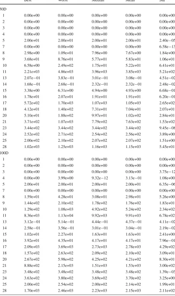
Table 12 CEC 2005 algorithms ranking
Rank nD=10 nD=30 nD=50
1 MP-AIDEA MP-AIDEA MP-AIDEA,npop=1
2 MP-AIDEA,npop=1 MP-AIDEA,npop=1 MP-AIDEA
3 G-CMA-ES (Auger and Hansen2005b) G-CMA-ES G-CMA-ES
4 L-SaDE (Qin and Suganthan2005) L-CMA-ES L-CMA-ES
5 DMS-L-PSO (Liang and Suganthan2005) K-PCX flexGA
6 L-CMA-ES (Auger and Hansen2005a) BLX-GL50
7 BLX-GL50 (García-Martínez and Lozano2005) SPC-PNX
8 DE (Ronkkonen et al.2005) DE (Ronkonnen)
9 SPC-PNX (Ballester et al.2005) DE (Bui)
10 EvLiv (Becker2005) flexGA
11 EDA (Yuan and Gallagher2005) CoEVO
12 K-PCX (Sinha et al.2005) EDA
13 BLX-MA (Molina et al.2005)
14 DE (Bui et al.2005)
15 CoEVO (Pošik2005)
16 flexGA (Alonso et al.2005)
17 ES (Costa2005)
6.2.2 CEC 2011 test set
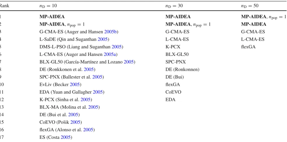
The results obtained on the CEC 2011 test set are reported in Table13. MP-AIDEA ranks first if problem 13 (the Cassini 2 Spacecraft Trajectory Optimisation Problem) is excluded from the test set and second if it is included.
The reason can be found in Fig.2. Figure2shows the con-vergence profile of the best solutions found by MP-AIDEA
and GA-MPC, the best algorithm of the competition, on function 13 for an increasing number of function evalua-tions (greater than the limit prescribed by the CEC 2011 competition). The results for GA-MPC are obtained using the code available online (http://www3.ntu.edu.sg/home/
epnsugan/index_files/CEC11-RWP/CEC11-RWP.htm).
Table 13 CEC 2011 algorithms
ranking Rank With function 13 Without function 13
1 GA-MPC (Elsayed et al.2011b) MP-AIDEA
3 MP-AIDEA GA-MPC
4 SAMODE (Elsayed et al.2011a) EA-DE-MA
5 EA-DE-MA (Singh and Ray2011) SAMODE
6 WI-DE (Haider et al.2011) WI-DE
7 Adap. DE 171 (Asafuddoula et al.2011) MP-AIDEA,npop=1
8 MP-AIDEA,npop=1 ED-DE
10 DE-Λ(Reynoso-Meza et al.2011) DE-Λ
11 ED-DE (Wang et al.2011) Adapt. DE 171
12 DE-RHC (LaTorre et al.2011) DE-RHC
13 RGA (Saha and Ray2011) RGA
14 Mod-DE-LS (Mandal et al.2011) Mod-DE-LS
15 mSBX-GA (Bandaru2011) mSBX-GA
16 ENSML-DE (Mallipeddi and Suganthan2011) CDASA
17 CDASA (Korošec and Šilc2011) ENSML-DE
Function Evaluations 105
0 2 4 6 8 10
Best Value
8.4 8.6 8.8 9 9.2 9.4 9.6 9.8
MP-AIDEA GA-MPC
Fig. 2 Best values of MP-AIDEA and GA-MPC for Function 13,
CEC2011
MP-AIDEA has a slower convergence for the first 200,000 function evaluations but then progressively finds better and better minima as the number of function evaluations increases. This demonstrates that in a realistic scenario in which function evaluations are not arbitrarily limited, MP-AIDEA would provide better results than the algorithm that won the competition.
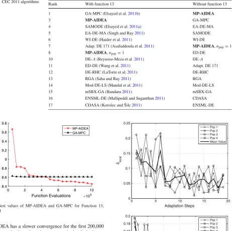
Results in Table13shows that MP-AIDEA with adapta-tion ofδlocalandnLRperforms better than MP-AIDEA with fixed values ofδlocalandnLR. The adaptation history ofδlocal is shown in Fig.3 for each of the four populations on test functions 12 and 13 and for 600,000 function evaluations.
6.2.3 CEC 2014 test set
The ranking results for the CEC 2014 test set are reported in Table14. MP-AIDEA with one population is tested in this
0 5 10 15 20
0 0.05 0.1 0.15 0.2 0.25
Adaptation Steps δ local
Pop 1 Pop 2 Pop 3 Pop 4 Mean Value
0 5 10 15 20 25 30
0 0.02 0.04 0.06 0.08 0.1 0.12 0.14 0.16 0.18 0.2
Adaptation Steps δ local
Pop 1 Pop 2 Pop 3 Pop 4 Mean Value
Fig. 3 δlocalfor the four populations of MP-AIDEA for functions 12
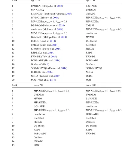
[image:16.595.82.545.60.519.2] [image:16.595.310.541.303.656.2]Table 14 CEC 2014 algorithms
ranking Rank nD=10 nD=30
1 UMOEAs (Elsayed et al.2014) L-SHADE
2 MP-AIDEA UMOEAs
3 L-SHADE (Tanabe and Fukunaga2014) GaPADE
4 MVMO (Erlich et al.2014) MP-AIDEAnpop=1, δlocal=0.1
5 MP-AIDEA,npop=1, δlocal=0.1 MP-AIDEA
6 DE-b6e6rl (Polakova et al.2014) CMLSP
7 rmalschma (Molina et al.2014) MP-AIDEAnpop=1, δlocal=0.3
8 MP-AIDEA,npop=1, δlocal=0.3 rmalshcma
9 GaAPADE (Mallipeddi et al.2014) MVMO
10 FERDE (Qu et al.2014) DE-b6e6rl
11 CMLSP (Chen et al.2014) b3e3pbest
12 b3e3pbest (Bujok et al.2014) FERDE
13 RSDE (Xu et al.2014) RSDE
14 FWA-DE (Yu et al.2014) FWA-DE
15 POBL-ADE (Hu et al.2014) POBL-ADE
16 OptBees (2014b) OptBees
17 SOO-BOBYQA (Preux et al.2014) SOO-BOBYQA
18 FCDE (Li et al.2014) NRGA
19 NRGA (Yashesh et al.2014) FCDE
20 SOO (Preux et al.2014) SOO
Rank nD=50 nD=100
1 MP-AIDEAnpop=1, δlocal=0.1 MP-AIDEAnpop=1, δlocal=0.1
2 UMOEAs UMOEAs
3 MVMO L-SHADE
4 MP-AIDEA MP-AIDEA
5 L-SHADE rmalshcma
6 MP-AIDEAnpop=1, δlocal=0.3 MP-AIDEAnpop=1, δlocal=0.3
7 rmalshcma POBL-ADE
8 b3e3pbest b3e3pbest
9 FERDE OptBees
10 DE-b6e6rl DE-b6e6rl
11 RSDE RSDE
12 POBL-ADE FWA-DE
13 OptBees
14 FWA-DE
15 SOO
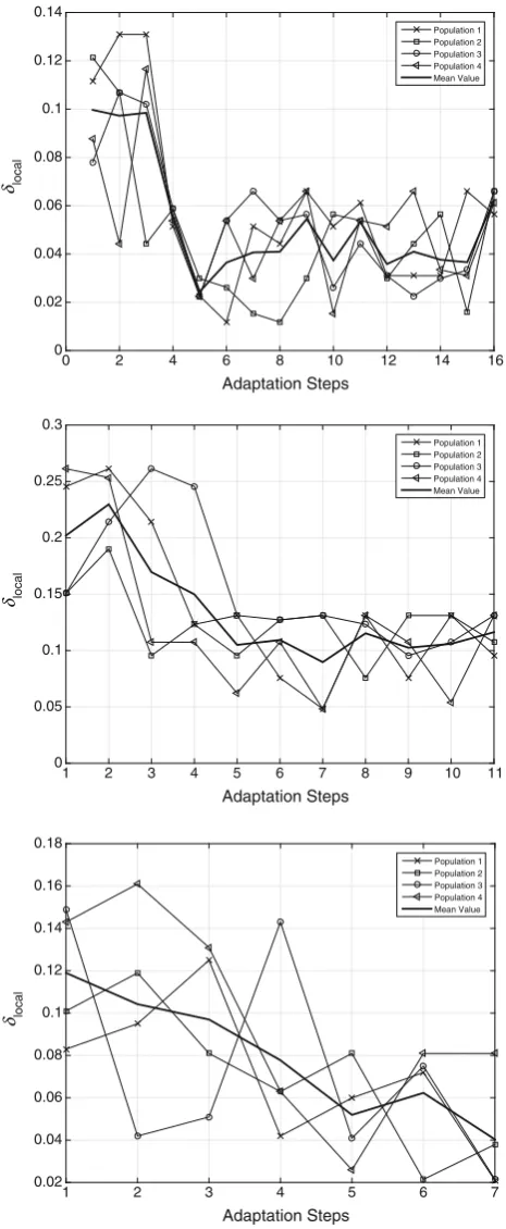
case withδlocal = 0.1 and δlocal = 0.3. FornD = 10 the results of MP-AIDEA with adaptation ofδlocal andnLRare better than those of MP-AIDEA with fixed values ofδlocaland
nLR, for bothδlocal=0.1 andδlocal=0.3. In the other cases MP-AIDEA with fixed values ofδlocalandnLRoutperforms MP-AIDEA with adaptation ofδlocalandnLRwhenδlocal= 0.1 but not whenδlocal =0.3. These results show the strong influence of this parameter on the results obtained by MP-AIDEA. The adaptation history ofδlocalfor test functions 9,
17 and 25 atnD =30 and 300,000 functions evaluations is shown in Fig.4.
Adaptation Steps 0
0.02 0.04 0.06 0.08 0.1 0.12 0.14
Population 1 Population 2 Population 3 Population 4 Mean Value
Adaptation Steps
δlocal
δlocal
δlocal 0 0.05 0.1 0.15 0.2 0.25 0.3
Population 1 Population 2 Population 3 Population 4 Mean Value
Adaptation Steps
0 2 4 6 8 10 12 14 16
1 2 3 4 5 6 7 8 9 10 11
1 2 3 4 5 6 7
0.02 0.04 0.06 0.08 0.1 0.12 0.14 0.16 0.18
Population 1 Population 2 Population 3 Population 4 Mean Value
Fig. 4 δlocalfor the four populations of MP-AIDEA for functions 9
(top), 17 (middle) and 25 (bottom),nD=30, CEC 2014
The performance of MP-AIDEA for the 30D functions of the CEC 2014 test set is further investigated to test the depen-dence of the results upon the two non-adapted parameters,ρ¯
andδglobal. Table15shows the raking obtained when varying
¯
ρandδglobal.
Case B of Table15shows the ranking obtained when using ¯
ρ = 0.3 instead thanρ¯ = 0.2. Comparing the results in Table15with those in Table14, it is possible to see that MP-AIDEA performs better usingρ¯ =0.3 rather thanρ¯=0.2, moving from the fourth to the third position in the ranking. At the same time, there is no significant dependence upon the value ofδglobal, as shown by Cases C and D in Table15, whereδglobalis changed from its nominal value of 0.1 to 0.2 and 0.3.
6.3 Wilcoxon test
The Wilcoxon rank sum test is a nonparametric test for two populations when samples are independent. In this case, the two populations of samples are, for each problem, thenruns values of the objective function obtained by MP-AIDEA and by another algorithms participating in the CEC 2011 and CEC 2014 competitions. No test is performed for the CEC2005 test set, since for no one of the algorithms partic-ipating in the CEC 2005 competition the code is available on-line.
The Wilcoxon test is realised using the Matlab®function
ranksum. ranksumtests the null hypothesis that data from two entriesxandyare samples from continuous distributions with equal medians. Results fromranksumare presented in the following as values of p andh. p, ranging from 0 to 1, is the probability of observing a test statistic as or more extreme than the observed value under the null hypothesis.
h is a logical value, whereh =1 indicates rejection of the null hypothesis at the 100α% significance level whileh=0 indicates a failure to reject the null hypothesis at the 100α % significance level, whereαis 0.05. Whenh =1, the null hypothesis that distributionsxandyhave equal medians is rejected, and additional test are conducted to assess which one of the two distributions has lower median. In order to do so, three types of tests are realised usingranksumfor the two distributionsxandy:
– Two-sided hypothesis test: the alternative hypothesis states thatx and y have different medians. Two distri-butions with equal medians will give as resultspB =1 andhB = 0 (failure to reject the null hypothesis that
x and y have equal medians), while two distributions with different medians will give as results pB = 0 and
hB=1 (rejection of the null hypothesis thatxandyhave equal medians). If the two-sided hypothesis test finds that the two distributions have equal medians (pB = 1 and
[image:18.595.54.287.55.621.2]