Observer based pulsed signal injection for grid impedance estimation in three phase systems

Observer-Based Pulsed Signal Injection for Grid

Impedance Estimation in Three Phase Systems

Pablo García,

Member IEEE, Mark Sumner,

Senior Member IEEE, Ángel Navarro-Rodríguez,

Student

Member IEEE, Juan M. Guerrero,

Member IEEE, and Jorge Garcia,

Senior Member IEEE

Abstract—This paper addresses the estimation of the grid impedance and the control of grid-tied converters by combining pulsed-signal injection and observer based techniques. A Luenberger based observer is used for con-trolling the grid-side current of an LCL filter by only mea-suring the converter-side currents and the grid-side volt-age. This configuration mitigates the effects of parameter variation at the LCL filter. Under grid impedance changes, the observer control signal will be used for triggering the signal injection. A Pulsed Signal Injection (PSI) approach is employed for estimating online the grid impedance using an RLS algorithm. Compared with existing grid-impedance estimation techniques, the proposed method can: 1) iden-tify a generic RL grid impedance, even under unbalanced conditions; 2) reduce the distortion induced by the excita-tion signal by relying on the observer to triggering the injec-tion when a grid impedance change is detected; 3) Identify grid impedance values much lower than the converter filter impedance, which is the usual situation when the converter rated power is well below the grid rating. Finally, it is worth pointing out that the proposed estimation technique is well suited to be incorporated into an adaptive current controller scheme.

I. INTRODUCTION

T

HE use of Voltage Source Converters (VSC) interfaced to the AC grid requires the control of the current delivered to the grid. In order to accurately design the current controller, it is critical to understand the dynamic model between the converter output voltage and the resulting grid current. The model will affect the converter performance in different ways, depending on the sensors used and the filter topology, i.e. L, LC, LCL, connecting the converter to the grid. When using an LCL filter for the interface, are several options for the placement of the current and voltage sensors, each one with their advantages and drawbacks [1], [2]. When AC voltage This work has been partially funded by the Campus of International Excellence (CEI) of the University of Oviedo, Spain, in the framework of Mobility Grants for Academics in 2013. Also partially supported by the predoctoral grants program Severo Ochoa for the formation in research and university teaching of Principado de Asturias PCTI-FICYT under the grant ID BP14-135. This work also was supported in part by the Re-search, Technological Development and Innovation Program Oriented to the Society Challenges of the Spanish Ministry of Economy and Competitiveness under grants ENE2013-44245-R, ENE2016-77919-R and by the European Union through ERFD Structural Funds (FEDER).

P. García, A. Navarro-Rodríguez, Juan M. Guerrero and J. García are with the Department of Electrical, Computer and System Engi-neering, University of Oviedo, Gijón, 33204, Spain (e-mail: garciaf-pablo@uniovi.es, navarroangel@uniovi.es, guerrero@uniovi.es, garcia-jorge@uniovi.es). Mark Sumner is with the Department of Electrical and Electronic Engineering, The University of Nottingham, University Park, Nottingham. NG7 2RD, UK. (email: Mark.Sumner@nottingham.ac.uk)

control at the converter output is needed, it is common to measure the voltage at the filter capacitor. However, this will make the current controller dynamics dependent on the grid side impedance [3]. An improved decoupling mechanism for the grid impedance variation can be implemented by placing the voltage sensor in the Point of Common Coupling (PCC). However, this will require either the measurement or the estimation of the capacitor voltage/current to effectively damp the current controller response [4]. This issue is more critical when the power converter is connected to weak networks having a non negligible grid impedance, thus affecting the total output impedance. In order to overcome this problem there are two different alternatives: 1) to force the known output filter to be the dominant dynamic system in any grid situation by implementing passive/active damping or virtual impedance techniques [5], [6], and, 2) to implement an adaptive current controller [7], [8], in which controller gains change depending on the grid impedance.

algorithm. The results are experimentally confirmed. However, all the electrical variables (grid current and voltages) need to be measured and operation under unbalanced conditions is not demonstrated. In [15], grid inductance is estimated using two consecutive samples of the grid current within a switching period. The estimation method is based on the discrete-time model at the grid frequency and, as recognized by the authors, the method is only valid for the inductive component. Moreover, the operation is only demonstrated for two different inductance values and unbalanced conditions are not considered.

Signal-injection based methods use an additional excitation in order to track the system response [16]–[23]. For the excitation signal, several approaches have been proposed: 1) Pulsed Signal Injection (PSI) [9], [23]–[25]; 2) High Frequency Signal Injection (HFSI) at constant high frequency [18], [19], [26]–[28]; 3) current regulator reaction [19]; 4) Low Frequency Signal Injection (LFSI) [20], [29], [30]; 5) Binary Sequence Signal Injection (BSSI) [21], [31], [32].

Regarding the PSI methods, the results presented in [9] are obtained in the absence of fundamental excitation and the pulses are injected period-to-period. The results in [24] are related to the ones presented in this paper, but they are only focused on a pure inductive three phase balanced impedance. The method proposed in [23] is based on param-eter identification using the pulse response and an adaptive model approach. The authors claim the method is able to estimate the grid admitance even with the presence of other power converters connected to the grid. The injected pulse magnitude and duration are similar to the one proposed in this paper. However, the activation of the pulse injection is not fully described and the results are only tested under real-time emulation provided by an OPAL-RT simulator. The method shown in [25] uses a current-pulse injection with the peak of the sinusoidal trajectory of 2 p.u. For the method proposed in our research, the peak pulsed current is around 0.03 p.u. Moreover, the use of the observer will allow the reduction of the current THD to below 1%. Furthermore, the signal processing is based on the DFT, increasing the computational burden and the memory requirements.

HFSI methods and current regulator reaction present some issues: 1) The selection of the high frequency requires the consideration of the possible reaction of any active power filter (APF) connected to the same PCC, compensating the high frequency voltage/current harmonics; 2) the estimated impedance is not the transient impedance, which determines the grid current response to the voltage changes imposed by the power converter, which is the one needed for current controller tuning.

LFSI methods can be separated into those adding an additional excitation signal, similar to HFSI methods, and those using the changes in the commands delivered by the power converter. Using the first approach, a current/voltage excitation signal of a given frequency, often an inter-harmonic, is injected into the grid. The grid voltage/current response at that frequency is analysed and the impedance at the injection frequency is obtained, often using frequency based methods. In [17], [29] a75Hz current signal is used. The same comments

as mentioned before for the HFSI methods apply: the distur-bance signal is continuously injected and the impedance is only estimated at the injection frequency. Additionally, due to the low-frequency signal injection, the reaction of the current regulators can compensate for the disturbance signal, thus reducing the effectiveness of the method. A solution given by the authors is to inject the excitation signal as a current reference, but then the bandwidth of the current controller can compromise the accuracy of the estimation. The second class of methods, require modifying the converter fundamental command. In [30], the P and Q commands are altered and both the inductive and resistive part of the impedance are estimated. The main drawback of this method is the coupling between the induced changes in the fundamental command used for the estimation from those due to the regular operation of the converter. The results are only verified by simulation and there is no discussion of the estimation under unbalanced conditions.

BSSI methods are based on the injection of a pulse-train who’s response is processed using frequency-based methods. They allow the grid impedance to be identified over a wide-range of frequencies. However, compared to PSI methods, they require a longer processing time because of the time required to inject the test signal and the calculations needed for the identification in the frequency domain. Moreover, most of the proposed methods are only validated for the estimation of the inductance term under balanced grid conditions.

In order to overcome the aforementioned problems, this paper proposes a hybrid strategy based on both an observer and a PSI. A Luenberger style observer will be used for controlling the grid-side current and detecting coarse grid impedance changes, only relying on the converter-side current and the voltage at the PCC. The proposed PSI, consisting of the injection of a pulse synchronized with the zero crossing of each three phase voltages, will allow the accurate measurement of the grid impedance by using a Recursive Least Square (RLS) algorithm. The proposed PSI method improves the THD when compared to other alternatives by constraining the injection of the pulses to those time intervals in which a change in the grid impedance is detected by the observer. As it will be demonstrated, the proposed technique allows for the estimation of both the resistive and inductive terms under unbalanced grid conditions. Thus, the contributions of this work can be summarized as: 1) identification of a generic RL grid impedance, including unbalance conditions; 2) reduction of the distortion induced by the excitation signal by relying on the observer to triggering the injection when a grid impedance change is detected; 3) identification of grid impedance values much lower than the converter filter impedance, which is the usual situation when the converter rated power is well below the grid rating.

shown in Section V.

II. SYSTEM MODELING AND CONTROL

A. System modeling

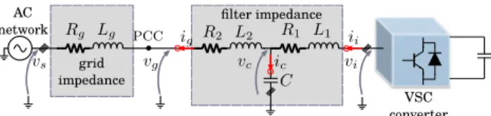
The state space representation of an LCL filter (Fig. 1) in an arbitrary reference frame is given by (1), (2); where x= [ii,vc,ig]

T

is the state vector and u = [vi,vg] T

the input vector, corresponding to the current and voltages in Fig. 1. Each component at the state and input vectors is a complex variable that can be split into the real,xx, and the imaginary, xy, parts. Equations (1) and (2) could be particularized for the stationary(α, β)or to the synchronous(d, q) reference frames by making ωe = 0 or ωe = ωgrid respectively. A compact representation is given at (3), (4). The corresponding block diagram using complex vector notation is shown in Fig. 2.

grid impedance

filter impedance AC

network

VSC converter

Fig. 1. Connection of the LCL filter to the output of the VSC.

Fig. 2. LCL filter block diagram in complex-vector form.

d dtxx=





−R1/L1 −1/L1 0

1/C 0 −1/C

0 1/L2 −R2/L2





x

·xx

+ωe





1 0 0

0 1 0

0 0 1



·xy+





1/L1 0

0 0

0 −1/L2





x

·ux (1) d

dtxy=





−R1/L1 −1/L1 0

1/C 0 −1/C

0 1/L2 −R2/L2





y

·xy

−ωe





1 0 0

0 1 0

0 0 1



·xx+





1/L1 0

0 0

0 −1/L2





y

·uy (2)

d

dtxx=Ax·xx+ωeI·xy+Bx·ux (3) d

dtxy=Ay·xy−ωeI·xx+By·uy (4)

B. Grid-side current observer

The superior filtering performance of the LCL structure when compared to the L or LC alternatives has also important shortcomings in the design of the current controller [33]. This situation is even worse when harmonic compensation is considered [34]. Current control using a LCL filter is a challenging task due to the resonance created by the capacitor and the inductances and often an attenuation method is needed. There are several alternatives in the literature which can be separated into passive and active damping techniques. On one side, passive damping techniques require the use of additional passive elements, such as series or parallel resistances which increase the system losses [33]. On the other, active damping methods often need for additional current or voltage sensors. Lately, some researchers have addressed active damping im-plementation methods not needing any extra elements [2], [35]–[40]. The methods in that group could be split in those requiring to estimate the capacitor current or the inductance voltage from those that rely on digital filtering of the control signal. The first approach requires the use of time derivatives which are normally noisy or require the use of complicated control algorithms. The second alternative places a notch filter at the current controller output, in order not to react at the LCL resonance frequency [35]. However, the bandwidth of the current controller must be often decreased.

In this paper, a control strategy based on a Luenberger type observer will be used [41]. The observer is similar to the one developed in [42], where direct discrete-time domain design is used instead. The simplicity of the design in the continous-time domain and the small difference in the performance for the parameters used in this research makes the solution in [41] appealing. It is also related with [43], but the more convenient converter side current is used instead of the grid side one. The proposed control strategy will estimate the grid-side current by using the converter-side current sensors and the voltage sensors at the PCC.

The observer-based current control block diagram is shown in Fig 3. The observer performance, at the synchronous reference frame, is shown at Fig. 4 when the estimated LCL filter parameters match the real ones. As shown, the grid current is correctly tracked and the dynamic performance is comparable to the one obtained when the grid side sensors are used. A detailed explanation about the working principles is provided in [41].

C. Digital control implementation

system plant

Observer

Fig. 3. Grid-current observer structure in an arbitrary reference frame.

time [s]

0 0.05 0.1 0.15

[A]

-10 -5 0 5

10 igd

m

ig_do iq_q ig_qo m

Fig. 4. Experimental results for the grid-current observer transient response. The results show a comparison of the observer-based control with respect to the sensor-based using an additional grid-side current sensor. Superscriptmis for the sensor-based control, whereasois for the observer-based control.

[k]and[k−1]correspond to the present and previous samples andTs is the sample time.

xx[k] =Kix·

Kax·xx[k−1]+

Ts

2 Bx ux[k]+ux[k−1]

+Ts 2 ωeI

xy[k]+xy[k−1]

(5)

xy_[k] =Kiy·

Kay·xy_[k−1]+ Ts

2 By

uy_[k]+uy_[k−1]

−Ts

2 ωeI xx[k]+xx[k−1]

(6)

whereKax,Kay,Kix,Kiybeing the values ofKa =I+T₂sA

andKi= I−T₂sA

−1

for either thex−ory−axes. The ob-server controller (Co) is also discretized using Tustin approx-imation. Proportional-Integral (PI) or Proportional-Resonant (PR) controllers can be selected depending on the implementa-tion being at the synchronous or the staimplementa-tionary reference frame respectively. In this study, a synchronous reference frame has been selected.

As explained in [41], the observer feedback signal, v_if b, reacts to any change in the grid impedance. That variation can be used for triggering the pulse injection, thus avoiding the injection of a continuous disturbance into the grid. Fig. 5 shows the experimental results when a sudden change in the grid impedance occurs for two different reactive current levels. As it can be seen, even if the changes in the fundamental command affect the observer signal, the variation due to the grid impedance change is for the shown cases more than100% larger.

0 0.05 0.1 0.15

0 2 4 6 8

0 0.05 0.1 0.15

0 6 14

0 0.05 0.1 0.15

0 2 4 6 8

0 0.05 0.1 0.15

0 8 19

Fig. 5. Experimental results for the transient detection. Top row: funda-mental grid currents components at the synchronous reference frame for two different current references,6and8. Blue color is used fordand red forq-axis. The transient at0.08seconds is due to the change of the grid impedance. Bottom row: observer feedback signal components at the synchronous reference frame. At each of the graphs representing the observer feedback signals, four traces are depicted. Blue and red colors are used for thedandqcomponents, respectively while magenta and yellow show the filtered signals with a2nd_{order Butterworth filter}

tuned with a cut-off frequency of 75Hz.

III. PULSEDSIGNALINJECTION

There are different PSI alternatives related with the injection parameters which can be adjusted. As shown in Fig. 6, the signal is centered at the zero crossing of the phase to neutral voltages. Zero crossing is detected by the PLL also used for grid synchronization. This instant has been selected in order to minimize the voltage distortion, as it will be discussed later.

pulse mag

pulse width 1 0 ph. u

ph. v ph. w

[V

]

0 5 10 15 20

−400 −200 0 200 400

time[ms] pulse width pulse mag

Fig. 6. PSI implementation. The pulse injection is synchronized and cen-tered with respect to the grid voltage zero crossing and the fundamental voltage command is blanked during the injection time. On the phase representation (ph.u, v, w), dashed lines show the starting and end of each phase pulse and solid ones the zero crossing of the respective phase.

but will also increase the resulting current THD. The values shown in Table I have been used. Resulting waveforms for the inverter commands and the applied voltages are shown in Fig. 7. The corresponding currents in the synchronous reference frame are depicted in Fig. 8. The three alternatives are described following:

1) Method#1. Pulse width is set to the desired value and the magnitude is set to zero. Under these conditions, the fundamental voltage command is clamped to zero during the pulse injection time. In the dq reference frame, even if the pulse is mostly applied at the q -axis, both components are modified. The pulses exhibit a triangular shape at theq-axis and the resulting current has a sinusoidal waveform.

2) Method#2. Fundamental command is held at the corre-sponding value at the beginning of the pulse injection and when the phase crosses the zero is changed to the symmetrical value with respect to zero. In thedq refer-ence frame,d-axis component is also affected, although in a less noticeable way than for Method#1. The pulses at theq-axis are also transformed to a triangular shape, but the resulting current has a triangular waveform of opposite phase when compared to previous method. 3) Method#3. Pulses are directly injected at the q-, d-,

or both axes by adding the pulses to the fundamental command delivered by the current controller. When compared to the pulse injection in the dq reference frame for both Method#1 and Method#2, the resulting excitation is stepwise in theabcreference frame but has triangular form in the dq reference frame. Even if the RLS algorithm is to be implemented in theαβreference frame, in order to allow the identification to work under unbalanced conditions it has been tested that the results are improved when square pulses are applied in thedq reference frame.

It must be remarked that all the pulse injection strategies share the fact that the applied distortion to the voltage com-mand is symmetrical with respect to the zero crossing, thus resulting in a zero average voltage error. Selecting one method or the other is based on the sensitivity of the current response and on the implementation burden. For this paper, Method#3 is considered, with the injection kept at theq-axis.

Experimental results of the system operating in closed-loop using the observer estimated grid current with a 500 Hz bandwidth are shown in Fig. 9. The results show that, even if the current controller reaction is affecting the pulses injection, they are clearly visible on the grid voltage and thus could potentially be used for the RLS estimation. It is also remarkable the close matching compared to the simulated results shown in Fig. 8. At this point, it is needed to

(V

)

-400 -200 0 200 400

(V

)

-400 -200 0 200 400

0 10 20

(V

)

-400 -200 0 200 400

0 10 20

Fig. 7. PSI waveforms for the three proposed methods in theabc refer-ence frame. From top to bottom, Method#1, Method#2 and Method#3. Left column shows the generated phase voltage command and right column the phase to neutral voltages. Dashed lines show the variables if the pulse injection is disabled.

comment on the additional THD distortion induced by the pulse injection. As it has been explained, pulse injection is disabled until a change in the impedance is detected by the observer. Whenever this happens, three pulses are injected (one at the zero crossing of each of the phases). The expected result is that the THD distortion is notably reduced with respect to existing techniques. In order to corroborate that, first a suitable procedure for the THD definition for pulsating signal has been carried out. As provided by the IEC61000-4-7 standard, ten fundamental periods of the voltage and current signals for 50Hz of nominal frequency are analyzed. Considering the pulsating and discontinous nature of the proposed injection mechanism, the THD is calculated in time domain using (7).

T HD[%] =

q

Pt=200ms

t=0 xsiαβ 2

q

Pt=200ms

t=0 xαβ2

·100 (7)

where xsi

αβ is the isolated injection voltage signal or the corresponding current response in theαβ reference frame and

(V

)

-100 0 100

(V

)

-100 0 100

0 10 20

(V

)

-100 0 100

(A

)

-2 0 2 4

(A

)

-4 -2 0 2

0 10 20

(A

)

-4 -2 0 2

Fig. 8. PSI waveforms for the three proposed methods in the dq reference frame. Fundamental component is removed in order to zoom on the injected pulsed components. Left column is for thevdqvoltages

and right for the idq current.d−axis andq−axis are represented in

blue and red respectively. From top to bottom, Method#1, Method#2 and Method#3.

v g

q[V]

-20 0 20

20 40 60 80

80 100 120

-10 0 10

a) time (ms) 0 20 40

i g

[A]

-2 0 2

b) time (ms) 0 20 40 2

4 6 8

c) time (ms) 0 20 40 8

10 12

d) time (ms) 20 -1

0 1

Fig. 9. Experimental results using Method#3. System is operated in closed-loop with a bandwidth of500Hz using the observed grid current. Top row shows theq-axis component of the grid voltage, whereas bot-tom row is for the observed grid current components in the synchronous reference frame. Different levels ofq-axis current commanded: a)0A, b)5A, c)10A, d) zoom for0A conditions. Blue color is used forq-axis component and red ford-axis. Att= 20ms, the2.4mH inductance series connected at the output of the LCL filter is changed to0.6mH.

carried out using the same simulation models, with same grid conditions and using the signal injection parameters as indicated by the authors. Results for the comparison are summarized in Fig. 10. As it can be seen, the proposed method has the lowest THD for the grid voltage, both for the 2ms and the 1ms cases. Considering the grid current THD, the proposed observer-based method is the second best for the 2ms case, just after the HFSI method, and the best one for the case of 1ms. It is also worth noting that the comparison conditions represent the worst case scenario for our proposal.

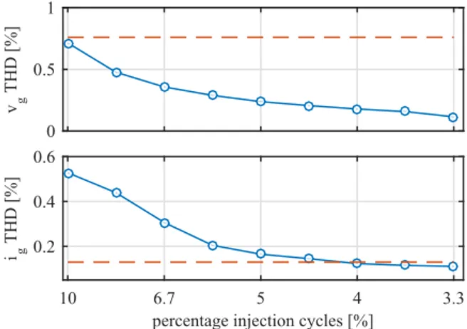
The calculated THD value assumes 3 pulses will be injected each 10 cycles, meaning that the observer is reacting to a change in the impedance each 10 cycles. However, the most important advantage of the observer-based method is the fact that the pulse injection is discontinuous, making the THD to be improved when the grid impedance is kept stable. Fig. 11 shows an interesting comparison between the observer-based injection and the HFSI method. There, the THD results for the2ms case are calculated as a function of the percentage of cycles in which the injection is applied. As it can be seen, the break-even point at which the proposed method improves the HFSI injection occurs when the ratio is lower than 4%. This condition is met after40grid cycles (0.8s).

v g

THD [%]

0 5 10

[17]

[18],[19] [21],[32] PSI cont PSI Obsv

i g

THD [%]

0 2 4

2

0.76 2.4

8

0.72

2.34

0.13 0.76 2.47

0.53 2.0

0.38 0.19

0.07

Fig. 10. THD comparison for the different methods analyzed in this paper. Both the grid voltage,vg and the grid current, ig are shown.

Numbers are for the references as cited in the bibliography. PSI cont. and PSI Obsv. are the continuous and observer-based pulse injection for two different pulses duration (blue for2ms and yellow for1ms).

v g

THD [%]

0 0.5 1

percentage injection cycles [%]

10 6.7 5 4 3.3

i g

THD [%] 0.2 0.4 0.6

Fig. 11. THD comparison for the PSI observer-based method (blue) and the HFSI method (dashed red) as a function of the percentage of cycles in which the injection is applied. Top, voltage at the PCC. Bottom, grid current.

IV. RLSALGORITHM IMPLEMENTATION

or estimators [27]. In this paper, the estimation of the system parameters is carried out by using an RLS approach [24], [44]. For that purpose, the differential voltage equation for the equivalent grid impedance in the stationary reference frame is discretized using Tustin method. The stationary reference frame is selected for the estimation in order to enable the system to work under unbalanced grid impedance conditions. In a stationary reference frame aligned with the spatial angle orientation of the impedance, each individual term contributing to the equivalent grid impedance as seen by the converter, i.e. cable impedance and loads, can be represented in matrix form by (8).

Z_{αβ i}=R_{αβ i}+jωeL_{αβ i}=

Z_ααi Z_{αβ i} Z_{αβ i} Z_{ββ i}

(8) In (8), theisubscript is related to each individual impedance seen from the PCC. When the impedance is balanced, Zααi equals Z_{ββ i}. Non diagonal terms (Z_{αβ i}) represent the cross coupling between phases. Rotating the impedance matrix to a common αβ reference frame and considering nimpedance elements, leads to (9).

Zαβ= n

X

i=1

ΣZi

1 0

0 1

+ ∆Zi

cosθie sinθie sinθei −cosθie

+

Z_{αβ i}

−sinθi

e cosθie cosθi

e sinθei

(9)

where ΣZi =

Zαα i+Zββ i

2 , ∆Zi =

Zαα i−Zββ i

2 , and θ

i e is the spatial angular phase of the unbalance impedance. For example, for single-phase loads at phases u, v, w, θie equals 0, 2π/3 or 4π/3 respectively. In the case the system is balanced, only the matrix terms depending on ΣZi will remain. The relationship with the phase impedances can be obtained by using the definitions: ΣZi = zai+zb₃i+zci and ∆Zi= zai+a·zbi+a

2_·zc i

3 , wherea=e

j2π/3_.

By considering the overall grid impedance dominated by the resistance and inductance terms, (9) can be expressed as (10).

Zαβ= n

X

i=1

(ΣRi+jωeΣLi)

1 0

0 1

+

(∆Ri+jωe∆Li)

cosθi

e sinθie sinθi

e −cosθie

+

(R_{αβ i}+jωeL_{αβ i})

−sinθei cosθie cosθie sinθei

(10)

where, ΣRi =

Rαα i+Rββ i

2 , ΣLi =

Lαα i+Lββ i

2 , ∆Ri = Rαα i−R_{ββ i}

2 , ∆Li =

Lαα i−L_{ββ i}

2 . From here, the voltage equation given by (11) can be obtained,

vzeqαβ=vgαβ−vsαβ=Rαβigαβ+Lαβ diαβ

g

dt (11)

where vzeqαβ is the voltage drop vector across the overall equivalent impedance, vgαβ and vsαβ are the PCC voltage and the grid voltage vectors (see Fig. 1), and igαβ is the grid current vector. Lαβ and Rαβ are, respectively, the sum of the inductance and resistance matrices for the different grid impedances as expressed in (10).

In the proposed estimation method, it is assumed that the

Lαβ is constant at the different harmonic frequencies, being the grid impedance the only variable affected by frequency according to (8) [45]. This has been experimentally validated by injecting harmonic components in the grid and measuring the corresponding harmonic impedance by calculating the Fast Fourier Transform (FFT) of the voltages and grid currents at the different frequencies. The results are shown in Fig. 12. As it is clearly shown, the inductance term remains almost constant aroundL= 0.5mH, whereas the impedance is clearly increasing with frequency due to the inductive behavior of the grid at that frequencies. At this research, none of the following effects are considered regarding the inductance variation: 1) inductance variation with saturation due to the fundamental command when the converter fundamental current is decou-pled from load variations, 2) variations due to parasitic effects such as skin, proximity, and parasitic capacitance effects and, 3) equivalent impedance in distribution grids dominated by active elements (power converters), being this last topic focus of attention of current research.

ω L [ Ω ] 0 2 4 [Hz]

150 _{350 450 550 650 750 850 9501050115012501350145015501650}

L [mH]

0 0.5 1

Fig. 12. Experimental results. Measurement of the harmonic impedance of the grid by injecting a distorted converter voltage. Voltages and currents at the PCC are measured and registered and the data is calculated in frequency domain. Sample rate is set to1Ms/s and spectral resolution is set to1Hz.

From (11), the discrete approximation for the grid current αβ components using Tustin method with a sampling period Tscan be expressed according to (12), (13).

iα_g[k] =aα₁ ·iα_g[

k−1]+a α 2 ·i

β g[k]+a

α 3 ·i

β g[k−1]

+bα₀ vα[k]+vα[k−1]

(12) iβg_[k] =a

β 1 ·i

β

g_[k−1]+a β 2·i

α g_[k]+a

β 3·i

α g_[k−1]

+bβ₀vβ_[k]+vβ_[k−1]

(13)

where aα 1 =

2

TsLαα−Rαα 2

TsLαα+Rαα, a α

2 = −

2

TsLαβ+Rαβ 2

TsLαα+Rαα, a α 3 = 2

TsLαβ+Rαβ 2

TsLαα+Rαα, b α

0 = 2 1

TsLαα+Rαα, a β 1 =

2

TsLββ−Rββ 2

TsLββ+Rββ, a β 2 =

−Ts2Lαβ+Rαβ 2

TsLββ+Rββ, a β 3 =

2

TsLαβ−Rαβ 2

TsLββ+Rββ, b β

0 = 2 1

From (12), (13) the values for the resistance and inductance terms can be obtained as (14).

Rxx= 1−ax

1

2bx 0

, Lxx= Ts

4 1 +ax

1

bx 0

,

Rxy=− ax

2+ax3

2bx 0

, Lxy= Ts

4 ax

3−ax2

bx 0

(14)

wherex,y could be eitherαorβ.

The RLS algorithm will allow to estimate the resistances and inductances in (14) by determining the values of the coefficients ax

i and bxj. The error driving the RLS update is obtained as the difference between the observed grid current, ix

g_[k], as calculated by the observer, and the one estimated by the RLS algorithm, ibxg_[k]. Decoupling of the unknown grid voltage, vαβ

s , is achieved by only considering the current induced by the pulse injection. This is done by subtracting the fundamental current reference from the overall current. It is then assumed that the grid voltage is stiff enough to neglect any effect on it due to the injected pulses and thus it could be removed from the equation.

The least squares problem is formulated in recursive form using the equations (15)-(18). The system equations are repre-sented by defining the variables and coefficients vectors,Xx

[k] , Wx

[k], as (19) and (20) respectively, where superscript x could be either α or β. The estimated RLS current, ibxg_[k], is determined by the product Wx

[k−1]·X x

[k] in (15). All the variables names are referred to those shown in Fig. 1.

α_[x_k] =ix_g

[k]−W x [k−1]·X

x

[k] (15)

g_[x_k] =Px_[k−1]·Xx_[k]·hλ+Xx_[k]T·P_[x_k−1]·Xx_[k]i

−1 (16)

Px_[k] =λ−1·Px_[k−1]−gx_[k]·Xx_[k]Tλ−1·Px_[k−1] (17)

W_[x_k] =W_[x_k−1]+αx_[k]·gx_[k]

T

(18)

Xx[k] = h

ixg_[k−1], iyg_[k], iyg_[k−1], vxg_[k], vxg_[k−1]

iT

(19)

Wx[k]= h

ax_{1 [k]}, ax_{2 [k]}, ax_{3 [k]}, bx_{0 [k]}, bx_{0 [k]}i (20) whereP(5×5)is the covariance matrix and it is initialized to

P= 0.01·I(5×5);g(5×1)is the adaptation gain, andλ= [0,1] is the forgetting factor, which need to be selected as a tradeoff of the expected estimation bandwidth and the signal to noise ratio. Values between 0.95 and1 are often selected. For this paper, the values shown in Table I have been used. After the injection of a new pulse, the estimation of theWcomponents for both the α and the β components is updated and a new estimation for Rαβ andLαβ is obtained using (14).

Regarding the computational burden of the proposed ap-proach, the number of needed floating operations have been determined by using a Matlab based tool. A total of 632 floating operations (multiplications and additions) are needed. Considering the number of cycles for each floating point op-eration based on a TMS320F28335 controller with a 150Mhz clock, it leads to a computational time lower than20µs. Thus, it is considered that the implementation is feasible and fast enough on medium performance digital signal controllers.

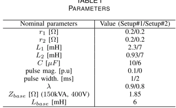
TABLE I PARAMETERS

Nominal parameters Value (Setup#1/Setup#2)

r1[Ω] 0.2/0.2

r2[Ω] 0.2/0.2

L1[mH] 2.3/7

L2[mH] 0.93/7

C[µF] 10/6

pulse mag. [p.u] 0.1/0

pulse width. [ms] 1/2

λ 0.9/0.8

Zbase [Ω] (150kVA,400V) 1.85

Lbase[mH] 6

V. SIMULATION ANDEXPERIMENTALRESULTS In order to illustrate the performance of the method under different balanced and unbalanced conditions, the simula-tion shown in Fig. 13 has been carried out. Different RL impedances have been connected in series between the output of the converter and the grid. Additionally, a balanced resistive load has been connected in parallel to the converter output. Every 0.1s, a transient is generated, changing the equivalent grid impedance. At t = 0.5s, an unbalance on the series impedance in phase-ais induced. Att= 0.7s, phase-a resis-tive load is reduced by 25%. Fast convergence and detection of asymmetries in theαandβ components are shown. Phase voltages at the PCC and estimated grid-side currents during the load transient are shown in Fig. 14. As clearly shown, the injection of the q−axis pulses is reflected at the PCC phase voltages and, consecuently, at the estimated grid-side currents.

Experimental results were obtained using a PM15F42C power module from Triphase. The power module is interfaced to the AC grid trough a LCL filter, which parameters are listed in Table I under Setup#1. Rated power of the converter is 15kVA, switching frequency is8kHz. The converter is coupled directly to the grid, without an isolation transformer. In Table I, L1 and L2 are the converter side and the grid side induc-tances respectively. For the experiments carried out, the L2 inductance is bypassed and the voltage is measured at the filter capacitor. The power converter running the RLS algorithm is connected to the grid by a set of different impedances, with inductance [0.5,1,2.5]mH ([0.0833,0.1667,0.4167]p.u) and resistance[0.2,0.15,0.15]Ω([0.1083,0.0812,0.0812]p.u). A 10Ω three-phase balanced resistive load is connected in parallel to the converter output. A picture for the experimental setup can be seen in Fig. 15. In order to check the accuracy of the method under a controlled environment, initial results have been obtained by disconnecting the grid and interfacing the converter to a balanced resistive load while varying the series impedance.

a)

v α

, v β

[V]

-500 0 500

b)

iα

, iβ

[A]

-20 0 20

c)

R α

, R

β

[

Ω

]

0 5 10

d)

Lα

, L

β

[mH]

0 2

e)

R α

β

[

Ω

]

-2 0 2

f) time (s)

0 0.2 0.4 0.6 0.8

L α

β

[mH]

-1 0 1

Fig. 13. Simulation results. Transient response. From top to bottom: a) vα, vβ. b) iα, iβ. c), d) Rαα,Rββ. and Lαα,Lββ

components for the matrices at the αβ reference frame. e) and f), the corresponding out-diagonal Rαβ and Lαβ. Every 0.1s

a new condition is evaluated by varying the equivalent phase resistances and inductances using the following sequence: Ra = [10.55,10.7,10.5,10.7,10.55,10.7,10.55,10.55]Ω,

La = [2.5,3,0.5,3.0,2.5,3.5,2.5,2.5]mH,

Rb = [10.5,10.6,10.4,10.6,10.5,10.5,10.5,10.5]Ω,

Lb = [2.5,3,0.5,3.0,2.5,2.5,2.5,2.5]mH, Rc =

[10.4,10.55,10.35,10.55,10.4,10.4,10.4,7.85]Ω, Lc =

[2.5,3,0.5,3.0,2.5,3.5,2.5,2.5]mH.Lbase= 6mH,Rbase= 1.85Ω.

load is also accurately determined, being the small variations on the resistance terms due to the changes of the associated inductance series resistances. The injected pulses in the αβ reference frame as well as the real and estimated currents are shown in Fig. 17. A good match between both signals can be observed.

Finally, experimental results with a grid-tied converter have been obtained. The method is tested with two different levels of reactive current, iq = [0,2.5]A. The commanded value of the fundamental current has been kept at low level compared to the converter rated current (30A) in order to analyze the perfor-mance of the current control when the pulses are injected. The grid voltages in Fig. 18 show a noticeable harmonic content, which will allow to demonstrate the operation of the method under distorted grid conditions. In Fig. 18, the grid voltages at the instant the three pulses are injected following a change in the impedance are shown. The effect of the pulse injection over the grid voltage is clearly visible, as well as the effect in the grid-side current.

Before the RLS estimation, the grid voltage and the fun-damental current are online decoupled. For the case of the voltage, the average value of the vd and vq components is subtracted. Being the pulse magnitude centered at zero, it does not affect the average value and thus the contribution

(V)

-400 -200 0 200 400

time (s)

0.65 0.7 0.75

(A)

-40 -20 0 20 40

Fig. 14. Simulation results. Transient response. On top the injected voltages by the converter at the PCC, on bottom the corresponding currents. The waveforms correspon to the same conditions explained in Fig. 13. Att= 0.7sthe load transient causes an unbalanced condition.

Power converter Variable filter

Resistances

Inductances

Fig. 15. Experimental setup. Photo for the Setup#1 describen in Table I. Left-side, a picture for the PM15F42C power module, at the right, a set of inductances used for the variable grid impedance, as well as the resistive loads.

of the grid can be easily removed. The resulting signal is rotated back to the stationary reference frame to be used in the estimation procedure. For the current signal, the current reference is subtracted from the overall current. Fig. 19 shows the estimation of the grid impedance during two different transients. The impedance values are filtered with a5Hz low pass filter to remove the high frequency noise affecting theai and bj values. As shown, the convergence of the method is really fast, arriving to the final value just after the injection of the last pulse.

VI. CONCLUSION

Rα , Rβ

[

Ω

]

0 5 10

L α

, L β

[mH]

0 1 2 3

Rα

β

[

Ω

]

-2 0 2

time [s]

0 5 10 15 20

Lαβ

[mH]

-1 0 1

Fig. 16. Experimental results. Transient response of the RLS algorithm. From bottom to top: a), b) the diagonal terms for the Rαα,Rββ and

Lαα,Lββ matrices at the αβ reference frame are shown. c), d) the

corresponding out-diagonalRαβandLαβ. A change is introduced into

the series impedance connected to phase a from 2.5mH to 0.5mH ([0.4167,0.0833]p.u) The small variations on the resistance terms cor-respond to the reistive changes due to the connection/disconnection of the inductances.

a)

vα

[V]

-50 0 50

b)

i α

(b), i

est α

(r)

[A]

-2 0 2

c)

vβ

[V]

-50 0 50

d) time (s)

6.785 6.79 6.795 6.8 6.805 6.81

i β

(b), i

est β

(r)

[A]

-5 0 5

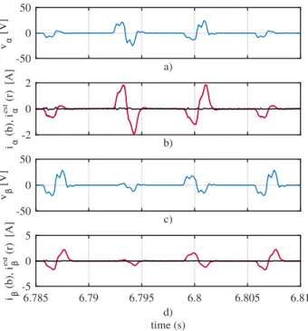
Fig. 17. Experimental results. Transient response of the RLS algorithm. a) and c) show a zoom on the injected pulses, whereas b) and d) show the corresponding grid-side current response. In b) and c) the measured and estimated current components are depicted in blue and red. Estimation error is depicted in black.

efficiency and the THD compared to other approaches relying on signal injection. The observer and the estimation method have been tested through simulation and experimental results. Different methods for the signal injection have been compared and the q-axis injection in the synchronous reference frame has been finally selected for an increased sensitivity. The RLS algorithm is implemented in the αβ reference frame to

[V]

-200 0 200

time [s]

26.52 26.54 26.56 26.58 26.6 26.62

[A]

-10 0 10

Fig. 18. Experimental results. Injection of the pulses when the power converter is connected to the grid. The upper graph shows the grid volt-ages and the lower one the corresponding grid currents. The converter was operated with a fundamental current commandiq= 2.5A.

[V]

-500 0 500

-500 0 500

[A]

-50 5 10

-50 5 10

Rα

, Rβ

[

Ω

]

-10 0 10

-10 0 10

Lα

, Lβ

[mH]

0 5 10

0 5 10

Rα

β

[

Ω

]

0 5 10

0 5 10

time [s]

33.44 33.46 33.48 33.5 33.52

Lαβ

[mH]

0 0.5 1

time [s] 36.52 36.54 36.56 36.58 0

0.5 1

Fig. 19. Experimental results. RLS results with the converter interfaced to the grid. From top to bottom: a) voltages at the filter capacitor. b) grid currents. c)Rα,Rβ. d)Lα,Lβ). e)Rαβ. f)Lαβ. The converter is current

controlled with a referencei∗q= 2.5A.

enable the operation both under balanced and unbalanced grid conditions. The proposed system is a suitable method for a different number of applications, including adaptive control, islanding detection and fault detection.

REFERENCES

[1] H. Xiao, X. Qu, S. Xie, and J. Xu, “Synthesis of active damping for

grid-connected inverters with an LCL filter,” in 2012 IEEE Energy

[3] J. He and Y. W. Li, “Generalized closed-loop control schemes with embedded virtual impedances for voltage source converters with lc or

lcl filters,”IEEE Transactions on Power Electronics, vol. 27, no. 4, pp.

1850–1861, April 2012.

[4] P. C. Loh and D. G. Holmes, “Analysis of multiloop control strategies

for lc/cl/lcl-filtered voltage-source and current-source inverters,”IEEE

Transactions on Industry Applications, vol. 41, no. 2, pp. 644–654, March 2005.

[5] W. Yao, M. Chen, J. Matas, J. Guerrero, and Z.-m. Qian, “Design and Analysis of the Droop Control Method for Parallel Inverters Considering

the Impact of the Complex Impedance on the Power Sharing,”IEEE

Transactions on Industrial Electronics, vol. 58, no. 2, pp. 576–588, 2011. [6] J. He, Y. W. Li, J. Guerrero, F. Blaabjerg, and J. Vasquez, “An Islanding Microgrid Power Sharing Approach Using Enhanced Virtual Impedance

Control Scheme,” IEEE Transactions on Power Electronics, vol. 28,

no. 11, pp. 5272–5282, 2013.

[7] M. Sumner, B. Palethorpe, and D. Thomas, “Impedance measurement for improved power quality-Part 2: a new technique for stand-alone active

shunt filter control,” IEEE Transactions on Power Delivery, vol. 19,

no. 3, pp. 1457–1463, 2004.

[8] J. Massing, M. Stefanello, H. Grundling, and H. Pinheiro, “Adaptive

Current Control for Grid-Connected Converters With LCL Filter,”IEEE

Transactions on Industrial Electronics, vol. 59, no. 12, pp. 4681–4693, 2012.

[9] Z. Staroszczyk, “A method for real-time, wide-band identification of the

source impedance in power systems,”IEEE Transactions on

Instrumen-tation and Measurement, vol. 54, no. 1, pp. 377–385, Feb 2005. [10] M. Sumner, B. Palethorpe, D. W. P. Thomas, P. Zanchetta, and M. C. D.

Piazza, “A technique for power supply harmonic impedance estimation

using a controlled voltage disturbance,”IEEE Transactions on Power

Electronics, vol. 17, no. 2, pp. 207–215, Mar 2002.

[11] M. Liserre, F. Blaabjerg, and R. Teodorescu, “Grid Impedance

Estima-tion via ExcitaEstima-tion of LCL -Filter Resonance,”IEEE Transactions on

Industry Applications, vol. 43, no. 5, pp. 1401–1407, 2007.

[12] A. Vidal, A. G. Yepes, F. D. Freijedo, O. López, J. Malvar, F. Baneira, and J. Doval-Gandoy, “A method for identification of the equivalent inductance and resistance in the plant model of current-controlled

grid-tied converters,” IEEE Transactions on Power Electronics, vol. 30,

no. 12, pp. 7245–7261, Dec 2015.

[13] A. K. Broen, M. Amin, E. Skjong, and M. Molinas, “Instantaneous frequency tracking of harmonic distortions for grid impedance

identi-fication based on kalman filtering,” in2016 IEEE 17th Workshop on

Control and Modeling for Power Electronics (COMPEL), June 2016, pp. 1–7.

[14] A. Bechouche, D. O. Abdeslam, H. Seddiki, and A. Rahoui, “Estimation of equivalent inductance and resistance for adaptive control of

three-phase pwm rectifiers,” inIECON 2016 - 42nd Annual Conference of the

IEEE Industrial Electronics Society, Oct 2016, pp. 1336–1341. [15] A. Ghanem, M. Rashed, M. Sumner, M. A. Elsayes, and I. I. I. Mansy,

“Grid impedance estimation for islanding detection and adaptive control

of converters,”IET Power Electronics, vol. 10, no. 11, pp. 1279–1288,

2017.

[16] D. Martin and E. Santi, “Auto tuning of digital deadbeat current controller for grid tied inverters using wide bandwidth impedance

identification,” in 2012 Twenty-Seventh Annual IEEE Applied Power

Electronics Conference and Exposition (APEC), 2012, pp. 277–284. [17] L. Asiminoaei, R. Teodorescu, F. Blaabjerg, and U. Borup, “A digital

controlled PV-inverter with grid impedance estimation for ENS

detec-tion,”IEEE Transactions on Power Electronics, vol. 20, no. 6, pp. 1480–

1490, 2005.

[18] D. Reigosa, F. Briz, C. Charro, P. Garcia, and J. Guerrero, “Active

Islanding Detection Using High-Frequency Signal Injection,” IEEE

Transactions on Industry Applications, vol. 48, no. 5, pp. 1588–1597, 2012.

[19] D. Reigosa, F. Briz, C. Blanco, P. Garcia, and J. Manuel Guerrero, “Active Islanding Detection for Multiple Parallel-Connected Inverter-Based Distributed Generators Using High-Frequency Signal Injection,” IEEE Transactions on Power Electronics, vol. 29, no. 3, pp. 1192–1199, 2014.

[20] L. Asiminoaei, R. Teodorescu, F. Blaabjerg, and U. Borup, “A digital controlled pv-inverter with grid impedance estimation for ens detection,” IEEE Transactions on Power Electronics, vol. 20, no. 6, pp. 1480–1490, Nov 2005.

[21] T. Roinila, M. Vilkko, and J. Sun, “Online grid impedance measurement

using discrete-interval binary sequence injection,” in 2013 IEEE 14th

Workshop on Control and Modeling for Power Electronics (COMPEL), June 2013, pp. 1–8.

[22] M. Cespedes and J. Sun, “Three-phase impedance measurement for

system stability analysis,” in2013 IEEE 14th Workshop on Control and

Modeling for Power Electronics (COMPEL), June 2013, pp. 1–6. [23] M. A. Azzouz and E. F. El-Saadany, “Multivariable grid admittance

iden-tification for impedance stabilization of active distribution networks,” IEEE Transactions on Smart Grid, vol. 8, no. 3, pp. 1116–1128, May 2017.

[24] M. Cespedes and J. Sun, “Adaptive control of grid-connected inverters

based on online grid impedance measurements,”IEEE Transactions on

Sustainable Energy, vol. 5, no. 2, pp. 516–523, April 2014.

[25] M. Céspedes and J. Sun, “Online grid impedance identification for

adaptive control of grid-connected inverters,” in 2012 IEEE Energy

Conversion Congress and Exposition (ECCE), Sept 2012, pp. 914–921. [26] M. Sumner, B. Palethorpe, and D. Thomas, “Impedance measurement

for improved power quality-Part 1: the measurement technique,”IEEE

Transactions on Power Delivery, vol. 19, no. 3, pp. 1442–1448, 2004. [27] N. Hoffmann and F. Fuchs, “Minimal Invasive Equivalent Grid

Impedance Estimation in Inductive #x2013;Resistive Power Networks

Using Extended Kalman Filter,”IEEE Transactions on Power

Electron-ics, vol. 29, no. 2, pp. 631–641, 2014.

[28] X. Guo, Z. Lu, X. Sun, H. Gu, and W. Wu, “New grid impedance

estimation technique for grid-connected power converters,”Journal of

Engineering Research, vol. 2, no. 3, p. 19, 2014. [Online]. Available: http://dx.doi.org/10.7603/s40632-014-0019-7

[29] L. Asiminoaei, R. Teodorescu, F. Blaabjerg, and U. Borup, “Implementa-tion and Test of an Online Embedded Grid Impedance Estima“Implementa-tion

Tech-nique for PV Inverters,” IEEE Transactions on Industrial Electronics,

vol. 52, no. 4, pp. 1136–1144, 2005.

[30] A. Timbus, P. Rodriguez, R. Teodorescu, and M. Ciobotaru, “Line Impedance Estimation Using Active and Reactive Power Variations,” in IEEE Power Electronics Specialists Conference, 2007. PESC 2007, 2007, pp. 1273–1279.

[31] A. Riccobono, S. K. A. Naqvi, A. Monti, T. Caldognetto, J. Siegers, and E. Santi, “Online wideband identification of single-phase ac power grid impedances using an existing grid-tied power electronic inverter,” in 2015 IEEE 6th International Symposium on Power Electronics for Distributed Generation Systems (PEDG), June 2015, pp. 1–8. [32] T. Roinila, T. Messo, and A. Aapro, “Impedance measurement of three

phase systems in dq-domain: Applying mimo-identification techniques,” in 2016 IEEE Energy Conversion Congress and Exposition (ECCE), Sept 2016, pp. 1–6.

[33] M. Liserre, F. Blaabjerg, and S. Hansen, “Design and control of an

LCL-filter-based three-phase active rectifier,”IEEE Transactions on Industry

Applications, vol. 41, no. 5, pp. 1281–1291, Sep. 2005.

[34] D. Wojciechowski, “Novel predictive control of 3-phase LCL-based

active power filter,” inCompatibility and Power Electronics, 2009. CPE

’09., May 2009, pp. 298–305.

[35] J. Dannehl, M. Liserre, and F. Fuchs, “Filter-Based Active Damping of

Voltage Source Converters With Filter,”IEEE Transactions on Industrial

Electronics, vol. 58, no. 8, pp. 3623–3633, Aug. 2011.

[36] M. Liserre, A. Aquila, and F. Blaabjerg, “Genetic algorithm-based design of the active damping for an LCL-filter three-phase active rectifier,” IEEE Transactions on Power Electronics, vol. 19, no. 1, pp. 76–86, Jan. 2004.

[37] S. Zhang, S. Jiang, X. Lu, B. Ge, and F. Z. Peng, “Resonance Issues and Damping Techniques for Grid-Connected Inverters With Long

Transmission Cable,”IEEE Transactions on Power Electronics, vol. 29,

no. 1, pp. 110–120, Jan. 2014.

[38] R. Pena-Alzola, M. Liserre, F. Blaabjerg, R. Sebastian, J. Dannehl, and F. Fuchs, “Systematic Design of the Lead-Lag Network Method for

Active Damping in LCL-Filter Based Three Phase Converters,” IEEE

Transactions on Industrial Informatics, vol. 10, no. 1, pp. 43–52, Feb. 2014.

[39] F. Huerta, E. Bueno, S. Cobreces, F. Rodriguez, and C. Giron, “Control of grid-connected voltage source converters with LCL filter using a

Linear Quadratic servocontroller with state estimator,” in IEEE Power

Electronics Specialists Conference, 2008. PESC 2008, Jun. 2008, pp. 3794–3800.

[40] M. Malinowski and S. Bernet, “A Simple Voltage Sensorless Active Damping Scheme for Three-Phase PWM Converters With an Filter,” IEEE Transactions on Industrial Electronics, vol. 55, no. 4, pp. 1876– 1880, Apr. 2008.

[41] P. García, J. M. Guerrero, J. García, A. Navarro-Rodríguez, and M. Sum-ner, “Low frequency signal injection for grid impedance estimation in

three phase systems,” in2014 IEEE Energy Conversion Congress and

[42] J. Kukkola, M. Hinkkanen, and K. Zenger, “Observer-Based State-Space Current Controller for a Grid Converter Equipped With an LCL

Filter: Analytical Method for Direct Discrete-Time Design,”Industry

Applications, IEEE Transactions on, vol. PP, no. 99, pp. 1–1, 2015. [43] C. A. Busada, S. G. Jorge, and J. A. Solsona, “Full-state feedback

equivalent controller for active damping in lcl -filtered grid-connected

inverters using a reduced number of sensors,”IEEE Transactions on

Industrial Electronics, vol. 62, no. 10, pp. 5993–6002, Oct 2015. [44] A. Arriagada, J. Espinoza, J. Rodriguez, and L. Moran, “On-line filtering

reactance identification in voltage-source three-phase active-front-end

rectifiers,” in The 29th Annual Conference of the IEEE Industrial

Electronics Society, 2003. IECON ’03, vol. 1, Nov. 2003, pp. 192–197 vol.1.

[45] F. Briz, P. García, M. W. Degner, D. Díaz-Reigosa, and J. M. Guer-rero, “Dynamic behavior of current controllers for selective harmonic

compensation in three-phase active power filters,”IEEE Transactions

on Industry Applications, vol. 49, no. 3, pp. 1411–1420, May 2013.

Pablo García (S’01-A’06-M’09) received the M.S. and Ph.D. degrees in electrical engineering and control from the University of Oviedo, Gijón, Spain, in 2001 and 2006, respectively. In 2004, he was a Visitor Scholar at the University of Madison-Wisconsin, Madison, WI, USA, Electric Machines and Power Electronics Consortium. In 2013 he was a visiting scholar at The University of Nottingham, UK.

He is the co-author of more than 20 IEEE journals and 50 international conferences. He is currently an Associate Professor within the Department of Electrical, Electronics, Computer, and Systems Engineering at the University of Oviedo. His research interests include control of grid-tied converters, parameter estimation, energy conversion, AC drives, sensorless control, AC machines diagnostics and signal processing.

Mark Sumner(M’92-SM’05) Mark Sumner re-ceived the B.Eng degree in Electrical and Elec-tronic Engineering from Leeds University in 1986 and then worked for Rolls Royce Ltd in Ansty, UK. Moving to the University of Nottingham, he completed his PhD in induction motor drives in 1990, and after working as a research assistant, was appointed Lecturer in October 1992. He is now Professor of Electrical Energy Systems.

His research interests cover control of power electronic systems including sensorless motor drives, diagnostics and prognostics for drive systems, power electronics for enhanced power quality and novel power system fault location strategies.

Ángel Navarro-Rodríguez(S’15) received the B.Sc. degree in telecommunications engineering with honors from the University of Castilla La-Mancha, Spain in 2012 and the M.Sc. degree in Electrical Energy Conversion and Power Sys-tems from the University of Oviedo, Gijón, Spain in 2014. Nowadays he is Ph.D student in the Department of Electrical, Computer, and Sys-tems Engineering in the University of Oviedo, granted by the government of Principado de Asturias.

He is part of the LEMUR research team in University of Oviedo since 2014 and his research interests include Energy Storage Systems, Control Systems, Electronics, Power Electronic Converters, Microgrids, power quality and Renewable Energies.

Juan M. Guerrero (S’00-A’01-M’04) received the M.E. degree in industrial engineering and the Ph.D.degree in Electrical and Electronic En-gineering from the University of Oviedo, Gijón, Spain, in 1998 and 2003, respectively.

Since 1999, he has occupied different teach-ing and research positions with the Department of Electrical, Computer and Systems Engineer-ing, University of Oviedo, where he is currently an Associate Professor. From February to Oc-tober 2002, he was a Visiting Scholar at the University of Wisconsin, Madison. From June to December 2007, he was a Visiting Professor at the Tennessee Technological University, Cookeville. His research interests include control of electric drives and power converters, smart grids and renewable energy generation.

Dr. Guerrero received an award from the College of Industrial Engi-neers of Asturias and León, Spain, for his M.E. thesis in 1999, four IEEE Industry Applications Society Conference Prize Paper Awards, and the University of Oviedo Outstanding Ph.D. Thesis Award in 2004.