Designing a Successful Trading Agent
for Supply Chain Management
Minghua He, Alex Rogers, Xudong Luo and Nicholas R. Jennings
School of Electronics and Computer Science, University of Southampton, U.K.
{
mh,acr,xl,nrj
}@ecs.soton.ac.uk
ABSTRACT
This paper describes the design and evaluation of Southampton-SCM, the runner-up in the 2005 International Trading Agent Sup-ply Chain Management Competition (TAC SCM). In particular, we focus on the way in which our agent purchases components using a mixed procurement strategy (combining long and short term plan-ning) and how it sets its prices according to the prevailing market situation and its own inventory level (because this adaptivity and flexibility are key to its success). We analyse our buying and selling strategies in the actual competition and in controlled experiments. Through this evaluation, we show that SouthamptonSCM performs well across a broad range of environments.
1.
INTRODUCTION
Effective supply chain management is vital to today’s economy and increasingly organisations are looking to the agility and automation afforded by agent-based approaches [4]. To this end, the Interna-tional Trading Agents Competition for Supply Chain Management (http://www.sics.se/tac) (TAC SCM) provides a benchmark-ing environment for testbenchmark-ing and evaluatbenchmark-ing agents in a challengbenchmark-ing and realistic setting. Specifically, in the TAC SCM scenario, the aim is to design an agent representing a computer manufacturer, that competes with other agents for computer components (from the supplier side) and computer orders (from the customer side). These agents are also responsible for managing their limited pro-duction capacities, in order to deliver the products to customers before the due date they agreed in the order.
In more detail, a game includes six agents (competition entrants) that compete with one another to procure raw components and ful-fil customer orders for assembled PCs. Each agent can produce 16 distinct computer types from four components: CPU, motherboard, memory and hard disk (e.g.a PC with a 2GHz IMD processor with 1GB memory and a 300GB hard drive). Consequently, on each of the 220 simulation days of the game, agents receive new request for quotes (RFQs) and actual orders (if offers they have previously sent win) from the customers. From the supplier side, an agent receives offers to deliver particular quantities and types of components at particular prices in response to the RFQs that it sent on the
previ-Permission to make digital or hard copies of all or part of this work for personal or classroom use is granted without fee provided that copies are not made or distributed for profit or commercial advantage and that copies bear this notice and the full citation on the first page. To copy otherwise, to republish, to post on servers or to redistribute to lists, requires prior specific permission and/or a fee.
Copyright 200X ACM X-XXXXX-XX-X/XX/XX ...$5.00.
ous day. Thus, in each day of the game (lasting 15 seconds), the agent must decide on the following: (i) which new supplier RFQs to send and which supplier’s offers to accept; (ii) which customer RFQs to respond to, and at what price; and (iii) how to schedule the production of PCs given the availability of components, the limited capacity of the factory and the delivery deadlines of pending orders. Now, an agent spends money on buying the components, paying for the storage of both components and PCs, paying penalties if it de-faults on a promised delivery date and paying overdraft penalties if it is in debt to the bank. The agent earns money by selling PCs and receives interest from the bank if its balance is positive. The success of an agent is measured in terms of its profit (i.e., its bank balance at the end of the game).
Against this background, we present the design and evaluation of our agent (SouthamptonSCM) that was the runner-up in the 2005 competition (out of 32 initial participants). The main contributions of this work are as follows. First, we develop techniques to enable the agent to adapt its price setting to the prevailing market situa-tion, its own internal state (inventory level) and the time that has elapsed. At their core, these techniques employ fuzzy reasoning in order to allow the agent to adapt its prices daily so that it can fully exploit its production capacity, while still maximising its rev-enue by selling at appropriate prices. Second, we develop a mixed procurement strategy that enables the agent to buy components ac-cording to what is needed in the near future (by predicting customer demand) and also to order a small quantity of components far in advance (at a lower price) to meet the minimum daily usage. This strategy balances flexibility in dealing with the dynamically chang-ing market, with the need to procure components at low cost whilst also minimising inventory stock. This is especially useful when the demand is increasing and the agents are thus competing for the components, since it is this case that causes component prices to increase. To evaluate the effectiveness of these developments, we analyse the performance of our agent in the actual competition and also in more systematic controlled experiments.
The remainder of the paper is organized as follows. Section 2 presents our agent. In section 3 we evaluate it. Finally, in section 4 we conclude and discuss future work.
2.
SouthamptonSCM
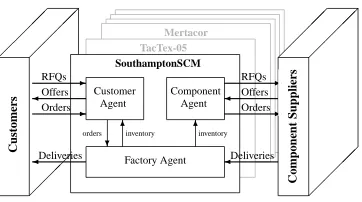
SouthamptonSCM is composed of three sub-agents (see figure 1).1 Thecustomer agentreceives RFQs from the customers and decides what offers to respond with. It also communicates with the fac-tory agent to obtain the updated invenfac-tory levels and to send the
1Here we use the notion of sub-agents (instead of modules) because
TacTex-05 Mertacor
6 6
?inventory inventory orders
SouthamptonSCM
Factory Agent Agent Customer
Agent Component
C
u
st
o
m
er
s
C
o
m
p
o
n
en
t
S
u
p
p
li
er
s
RFQs Offers Orders
Deliveries
RFQs Offers Orders
[image:2.612.83.264.51.152.2]Deliveries
Figure 1: SouthamptonSCM agent architecture.
relevant customer PC orders. Thecomponent agentdecides which RFQs and which orders to send to which suppliers. Thefactory agentreceives the supplies delivered from the suppliers, decides based on the available resources (computer components and fac-tory cycles) in what order the customer orders should be produced, and determines the schedules for delivering the finished PCs to the customers. We now deal, in turn, with each sub-agent.
2.1
The Customer Agent
The customer agent is the key component in our architecture (be-cause we believe that offering the appropriate price at the right time is vital for success). If the price is too low, the agent will receive a low profit and if it is too high it will fail to win any orders (because customers always choose the lowest offer price among those they receive). Given this, the key challenges are to determine which customer RFQs to bid for and at what price. To achieve this, we use fuzzy reasoning to determine how to set prices according to the agent’s inventory level, the market demand and the time into the game. Moreover, the parameters involved in the fuzzy rules can be adapted according to the quantity of the received and expected customer orders so as to maximise the factory utilisation.
The customer agent we used in last year’s competition has pre-viously been described in [3] and in several respects this year’s de-sign is similar. However, due in part to the changes in the rules of this year’s competition and also because SouthamptonSCM 2005 is built upon last year’s experiences, there are also a number of important differences. Most importantly:
• When prioritising customer RFQs, SouthamptonSCM 2005 considers the potential profit that each RFQ will generate (SouthamptonSCM 2004 did not consider the cost of the com-ponents). Moreover, when checking on the availability of the components required to assemble the requested finished product, unlike SouthamptonSCM 2004 that just considered the quantity of components held as inventory, the 2005 agent also considers pending component orders that are due to be delivered before the due date of the RFQ (see Section 2.1.1).
• SouthamptonSCM 2005 also calculates the offer prices of finished products differently. Although it uses the same ba-sic technique as the 2004 agent, the 2005 agent has two rule bases for calculating prices: one for when it is close to the end of the game and one for other days in the game (see Sec-tion 2.1.2). The 2004 agent, also used two rule bases but these were: one for the end stage of the game and one for when it was expecting a large component delivery.2
2This rule was motivated by the use of a day 0 procurement strategy
that ordered the majority of the components needed for the entire game on day 0. Since changes in the TAC SCM game specification for the 2005 competition removed the benefit of this procurement strategy, the customer agent had to be updated.
We now deal, in turn, with each of the these differences.
2.1.1
Choosing Customer RFQs.
The customer agent receives customer RFQs requesting a quantity of a particular PC for delivery on a specified day. When selecting which RFQs to respond to, SouthamptonSCM rates them accord-ing to the potential profit that they may braccord-ing and accordaccord-ing to the inventory it holds. The latter inventory driven strategy offers cus-tomers PCs according to what is currently available and also what can be produced given the delivery date of pending components or-ders. This consideration of promised component deliveries is new and is included this year since changes to the supplier model mean that there are no longer significant delivery delays in these compo-nent orders3[1].
In more detail, suppose a customer RFQ is represented as a tuple (i,q, pres,cpenalty,ddue), wherei∈ {1,· · ·,16}is the type of PC
the customer wants,q>0 is the quantity,pres>0 is the reservation
price (maximum it will pay), cpenalty>0 is the fine paid if the
computers are not delivered on time, andddueis the desired delivery
date. On each day, the customer agent receives a bundle of such RFQs and sorts them in the decreasing order of the profit margin of the type of PC requested:
pres−pbase− cpenalty
q ,
wherepbaseis the cost of buying components (sum of the buying
price for each component). The intuition is that the agent will first serve customers with high profit margins and low penalties. This is because the higher thepres, the more profit will be made (compared
to selling the same product to a customer with a lowpres). At the
same time, the agent also wants to avoid getting high penalty orders because of the inherent uncertainties that exist in the game.
For each RFQ in the list, the agent first checks whether it can be supplied from its stock of finished PCs (see Section 2.3). If it can, the corresponding PC inventory is decreased. Otherwise, the agent checks whether it holds sufficient components within both its current inventory and its expected delivery queue (i.e.components that have been ordered, but have not yet arrived), and also whether it has a sufficient remaining production capacity to manufacture the required PCs. If it does, the agent decreases its available compo-nent inventory.
2.1.2
Fuzzy Rules for Calculating Offer Prices
For each type of PC, the agent uses a fuzzy reasoning inference mechanism which is based on the standard Sugeno controller [6] to calculate the offer price of components. Full details of this process are described in [3], however, here we present the rule bases as used in the 2005 agent. Now, due to the constraint that the TAC SCM game is played over a fixed number of days, we use two rule bases: one for the majority of the game days where the aim is to sell fin-ished products at maximum profit, and one for the last stages of the game where the aim is to ‘off-load’ any remaining finished prod-uct and component inventory. Splitting the rule bases enables us to reduce their complexity and thus maintain their interpretability.
In more detail, in the first rule base, for each PC type the agent considers the current customer demand state and the inventory level of the components that make up that particular PC type. There are twelve such rules within this base and the following three are representative examples:
R
1: ifDishighandIislowthenr1isvery-big3These changes were introduced to remove the incentive to adopt a
RFQ RFQ RFQ RFQ RFQ Orders Offers
C
o
m
p
o
n
en
t
S
u
p
p
li
er
s
Component Agent
Offer Processing
Near Future Procurement
Far Future Procurement Demand Predictor
[image:3.612.82.268.52.159.2]Price Tracker
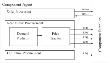
Figure 2: Overview of the component agent.
R
2: ifDismediumandIishighthenr2isvery-mediumR
3: ifDislowandIishighthenr3issmallIn these rules, the customer demand (D) is expressed in the fuzzy linguistic termshigh,medium, andlow, and the inventory level (I) in the termshigh,medium, andlow. The output of each rule is a fuzzy variable (r1 tor3 in these examples), and thus, the outputs
of all the rules are combined by the Sugeno controller to give a single scalar result,r, that represents theprice adjustment factor used to generate a reference price [2] for each type of PC. When ris high, the reference price approaches (or is even higher than) the highest transaction price recorded on the previous day (this in-formation is made available to the agents through the daily market report), whilst whenris low, the reference price approaches the lowest transaction price. Given the reference price of each type of PC, an offer price is calculated by modifying the reference price by a factor related to the requested due date. The intuition here is that the sooner the due date, the higher the offered price. Thus, rule
R
1captures the fact that if the customer demand for this kind of PC is high and the agent has a low inventory in stock, then the offer price should be very high since here there is an opportunity to maximise the agent’s profit.
The second rule base is employed for the days near the end of the game (last 20 in this case) and it considers the current inventory level, the customer demand and also how close it is to the end of the game. There are 22 such rules that capture different combinations of situations of these three variables, and, three such rules in this rule base, are:
R
10: ifDishighandIishighandEisf arthenr0
1isbig
R
20: ifDishighandIishighandEismediumthenr0
2ismedium
R
30: ifDislowandIishighandEisclosethenr0
3isvery-small
Here, the days to the end of the game (E) are expressed in the fuzzy linguistic terms: far,medium, andclose. Thus, for example, rule
R
30 captures the fact that if there is little demand for a particulartype of PC, the agent has a high inventory, and there is a little time until the end of the game, then the price adjustment factor should be very small (thus ensuring a low offer price and hence reducing the risk of being left with inventory at the end of the game).
2.2
The Component Agent
The component agent is responsible for dealing with the compo-nent suppliers and aims to ensure that there are always sufficient components in stock to address the customers’ changing demand for finished products. In doing so, it addresses a challenge that is common to all supply chains facing dynamically changing cus-tomer demand. That is, it must procure components at a low cost, whilst simultaneously maintaining a minimal component inventory in order to reduce the daily storage cost and also the possibility of being left with redundant stock if customer demand changes.
Now, the 2005 component agent uses a completely different strat-egy to that of last year. In 2004, it procured most of its components by placing a large order on day 0 (due to the fact that the suppli-ers have their full capacity available on day 0 and thus offer the lowest possible price [3]). However, in 2005, the game rules were changed in order to reduce the lottery effect in the supplier inter-actions, to discourage the use of a day 0 procurement strategy [7], and to deter agents from requesting large quantities of components without intending to order them [1]. This means that the compo-nent agent used in 2004 is no longer effective, and thus, we present our updated component agent here.
In addressing the procurement challenge this year, the agent faces a common dilemma concerning the lead time of component orders. More specifically, ordering components with a long lead time (i.e. for delivery a long time into the future) generally leads to low pro-curement costs (since the suppliers have adequate spare capacity over this long period). However, the agent is then exposed to the risk that the customer demand may change, leaving it with exces-sive component stock. Conversely, ordering components with a short lead time allows the agent to effectively track the changing customer demand and maintain minimum stock inventory. How-ever, due to the short lead time, the suppliers generally have less flexibility in scheduling the production of these orders (since the order is competing with those from other agents for the limited pro-duction capacity available), and thus, procurement costs are high.
Now, to tackle this dilemma, SouthamptonSCM employs a mixed procurement strategy; dividing the remaining days of the game into two classes: near future and far future (see figure 2). For the days in the far future, the agent periodically orders a small fixed quantity of components, so as to ensure that a minimum quantity of stock is available in order to keep the factory running (see section 2.2.1 for details). For the days in the near future (which is 35 days in this case4), the agent makes a short term prediction of the future cus-tomer demand, and orders sufficient components to address this de-mand (see section 2.2.2 for details). In addition, within this near fu-ture, the agent alsoteststhe market in order to track current prices. This price information is used to choose the appropriate lead time and reserve price of the RFQ sent to the suppliers. In more detail, since each agent can send a maximum of five RFQs for a particu-lar component to each supplier each day, the agent uses four RFQs for the near future procurement (i.e. to actually order components with short lead time and also to track the component prices). The remaining RFQ is used to buy components for the far future.
2.2.1
Far Future Procurement
Of the two strategies, the far future procurement one is the simpler. For this, the agent assumes that in the far future, there will be a daily minimum need for 30 CPU and 60 other components (this ratio is required since there are four different types of CPU, but other com-ponents are only available in two different types), and thus checks whether there is sufficient current and pending component inven-tory to meet this need. If not, it submits an RFQ for a fixed amount to the relevant supplier, requesting delivery on the date at which the predicted inventory falls below the daily minimum need (up to a maximum of 120 days into the future).
2.2.2
Near Future Procurement
The near future procurement strategy is more complex. It
con-4In our experimental evaluation, we found that a larger number
6
-d+n d
d−x days
log(Nd)
log(Ndˆ+n)
log(Qdˆ)
aa aa
aa a
aaa a
@ @ I
[image:4.612.91.255.52.152.2]Daily number of RFQs
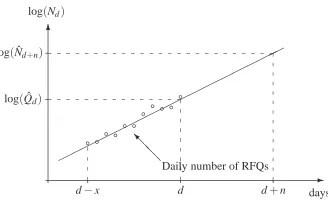
Figure 3: Linear regression process by which Southmapton-SCM predicts the future customer demand.
sists of two elements, a daily demand predictor that predicts the future demand of components, and a market tracker that generates the RFQs to be sent to the suppliers, both to order actual compo-nents required and to test the market to discern the most profitable order lead time and set appropriate reserve price.
Demand Predictor
As described above, the agent buys components for the near fu-ture based on a prediction of customer demand. Now, according to the game specification, the number of RFQs that each agent re-ceives from the customers is described by three independent ran-dom walks; one for each market segment (finished product PCs are classified into three such segments: high, mid and low range). In more detail, the number of RFQs that an agent receives, within a single market segment, on daydis denoted byNd, and is drawn
from a Poisson distribution whose expected value is given by the parameter,Qd. Thus, for each market segment:
Nd=Poisson(Qd) (1)
Again, according the game specification, the value ofQdis updated
each each day between minimum and maximum limits according to a multiplicative trend parameter,τd, and thus:
Qd+1=min(Qmax,max(Qmin,τdQd)) (2)
where the trend,τd, is itself updated each day, again between
min-imum and maxmin-imum limits, according to a random walk:
τd+1=max(τmin,min(τmax,τd+random(−0.01,0.01))) (3)
Now, sinceτdvaries relatively slowly (and can thus be assumed to
be constant over short periods of time), the agent can estimate the values ofQdandτd(these estimated values are denoted by ˆQdand
ˆ
τd) by recording, for the previousxdays, the number of RFQs
re-ceived within each market segment (i.e. Nd−x. . .Nd), and then
per-forming a linear regression of the logarithm of these values against d(we take the logarithm since the trend is multiplicative). Having found these values, the agent can then extrapolate, and predict the number of RFQs that will be received on dayd+n, and thus:
ˆ
Nd+n=min Qmax,max Qmin,(τˆd)nQˆd
(4)
This process is shown diagrammatically in figure 3. In trials, we found that by using data from the previous 10 days, and predicting a value for 10 days into the future (i.e. x=10 andn=10), we obtained a good estimate for the average demand within the near future. This process gave significantly better results than the simple alternative of using the number of RFQs received on the current day, as an estimate for future days.
Having predicted the number of RFQs that will be received, within each market segment, on each day within the near future, the agent then calculates the expected daily usage of each component type
(Did). This is calculated by weighting the maximum number of
PCs that can be manufactured on any day,Dtotal,5by a factor that
incorporates both the expected number of RFQs that will be re-ceived within each market segment (i.e. Nˆlow
d+n, ˆNdmedium+n and ˆN high d+n
as described above) and a weighting that describes how many of the PC types within any market segment actually contain the specific component being considered (for any component this weighting is described byridlow,rmediumid andrhighid and, for example, for compo-nent id of 200 these values are 0.4, 0.5 and 0.6 respectively). Thus:
Did= Dtotal
h
ridlowNˆdlow+n+ridmediumNˆdmedium+n +rhighid Nˆdhigh+ni
ˆ
Ndlow+n+Nˆmedium
d+n +Nˆ
high d+n
(5)
GivenDid, the current available stock of each component, and
the expected deliveries from the suppliers from previous orders, the agent checks whether stock levels in the near future will fall below a minimum threshold. This threshold represents a buffer stock level, and guided by the principle that towards the end of the game the inventory level should decrease, it starts from 0 on day 0, increases gradually to a fixed number of 300 CPU and 600 other components over the first 30 days, and subsequently decreases to zero again over the last 10 days. If stock levels are predicted to fall below the buffer level within the near future, the agent identifies the quantity required (with a maximum order size of 80 components) and the latest date that this quantity should arrive by. This information is passed to the price tracker, which actually generates the RFQs that are sent to the suppliers.
Price Tracker
The price tracker acts to maintain an estimate of the current market price of the components. Due to the behaviour of the competing agents, this market price depends on the due date with which com-ponents are requested. For example, if the competing agents are ordering components with very short lead times, then the supplier will have little spare capacity, and thus, the corresponding offer prices that the agent receives will be greater than those of orders with long lead times. Every day the the price tracker generates four RFQs which are sent to each supplier. The due dates of these RFQs are distributed over three regions within the near future (i.e. less than 10, 10 to 20, and more than 20 days into the future) and the offer price that the agent receives in response to these RFQs en-ables it to track the changing market price of the component and also to identify the order lead times that will result in the minimum procurement costs.
Now, in more detail, the four RFQs generated by the price tracker fall into two different classes: those that actually order the compo-nents requested by the demand predictor, and those that have zero quantity (and are simply used to track the market price). On any day, up to four of these RFQs will be used to actually order com-ponents (depending on the requirements of the demand predictor), and within the constraints of the delivery date requested by the de-mand predictor, the lead time of these RFQs will be determined by the results of the market testing. This market testing is also used to set an appropriate reserve price for the RFQ.6
5In this case,D
total=364, since, given the factory production
ca-pacity of 2000 cycles per day and an average production cost for a PC of 5.5 cycles, approximately 2000/5.5=364 PCs can be man-ufactured per day.
6Note, the setting of this reserve price is particularly important in
0 40 80 120 160 200 0
0.5 1 1.5 2
x 105 Cumulative Order Quantity (cycles)
Simulation Day
[image:5.612.93.251.51.192.2]SouthamptonSCM TaxTex−05 Mertacor
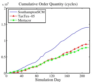
Figure 4: Cumulative order quantities in game tac4-4253.
2.3
The Factory Agent
One of the main challenges for the factory agent is scheduling what to produce and when to produce it (i.e., how to allocate supply re-sources and factory time). The strategy we use for Southampton-SCM 2005 agent is broadly similar with that of last year’s agent. This strategy involves manufacturing PCs according to customer orders and satisfying orders with an earlier delivery date (see [3] for more detail). Now, since the computers stored in the factory will be charged storage cost, each order will be delivered as soon as it is filled. The agent builds the PCs according to the customers’ orders it has obtained (which has the advantage of ensuring that the factory always produces the needed computers on time). How-ever, if on any day, there are still free factory assembling cycles available, and the numbers of finished PCs in stock are below a certain threshold, then the agent produces additional PCs of each kind uniformly (subject to the availability of components) in order to maximise the factory utilisation. It is critical that this threshold is set appropriately; a high threshold will lead to excessive finished PC inventory, which may be hard to sell if demand is low. In 2005, this threshold is set to 80, and this is shown to work well in both low and high demand markets.
3.
EVALUATION
Our evaluation is composed of three components: (i) the results from the 2005 competition; (ii) our post-hoc analysis of some typi-cal games in the actual competition; and (iii) a systematic range of controlled experiments.
3.1
Competition Results
TAC SCM consists of a preliminary round (predominantly used for practice and fine tuning) followed by a seeding round that deter-mines the groupings for the final rounds. The top 24 agents from the seeding round are organised into 4 groups that represent each of the four quarter-finals. The top three teams of quarter-finals 1 and 3 are entered into semi-final 1, and similarly, the first 3 teams from quarter-finals 2 and 4 are entered into semi-final 2. Finally, the first 3 teams in both semi-finals are entered into the final round.
In the 2005 competition, there were 32 entries and Southampton-SCM was placed seventh among all the participants in the seeding
are placed. Agents with higher reputation are given priority treat-ment and receive lower offer prices. Thus SouthamptonSCM main-tains a perfect reputation record by adopting the policy of accepting all offers that it receives (this is dealt with by theOffer Processing in figure 2). Thus, it is essential that the agent sets the reserve price of RFQs to an appropriate value, to avoid being obliged to accept an excessively expensive offer.
round and entered group B for the quarter-final. Here, it had the second highest score, in its semi-final it had the highest score, and in the final, it was the runner-up (to TacTex-05 [5]).7
3.2
Competition Game Analysis
In this section, we analyse the performance of SouthamptonSCM in terms of the efficiency of both its buying and selling strategies. That is, we consider the effectiveness of the customer pricing model and the mixed component procurement strategy. Thus we select a particular game from the final (game tac4-4253) and analyse it in more detail.8
3.2.1
Analysing the Selling Strategy
To complement and better understand the competition result and to evaluate the effectiveness of our pricing model (since we attribute our success in selling PCs to the pricing technique we employ), we conducted a post hoc analysis of a game from the final. In order to reduce the complexity of this analysis, we consider just the top three performing agents within this game (i.e. in this case SouthamptonSCM, TacTex-05 and Mertacor (who also happen to be the top 3 agents in the overall competition)). Now, an essential factor in the performance of the trading agent is the ability to re-spond to customer RFQs with competitive offer prices. Thus, we analyse the game data and we consider just those RFQs for which all three of the above agents responded with offers. We then con-sider which of the three agents actually won these orders (noting that the order is always assigned to the agent that offers the lowest price). In figure 4 we show the resulting order quantities (expressed as factory production cycles averaged over all products), that were won by each of the three agents. Significantly, the Southampton-SCM agent wins a far larger proportion of the orders than the other two agents. This is consistent with the overall game analysis, where the orders these three agents delivered in the game are: 7331 for SouthamponSCM, 6742 for TacTex-05, and 5588 for Mertacor.
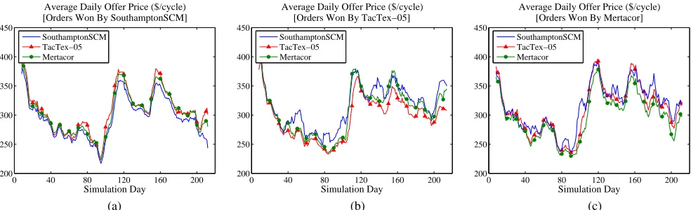
Now, there is little advantage to win these orders, if the offer price was excessively low. Thus, in figure 5, we compare the av-erage offer prices for those orders that were won by each of the three agents. Specifically, in figure 5a we show the average offer prices of the orders that were actually won by SouthamptonSCM, in figure 5b those won by TacTex-05, and in figure 5c those won by Mertacor. In each case, as expected, we see that the agent that won the orders actually submitted offers with the lowest average price. However, despite winning the majority of the orders, the prices offered by SouthamptonSCM were not significantly lower than those of the other agents. Indeed, the opposite is true. The margin by which SouthamptonSCM undercut the other agents is actually smaller than the margin with which the other agents un-dercut SouthamptonSCM. For example, in this game, on average SouthamptonSCM undercut Mertacor’s prices by 3.0% and TaxTex-05’s prices by 4.1%. Conversely, on average, TacTex-05 under-cut SouthamptonSCM’s prices by 6.5% and Mertacor underunder-cut the prices of SouthamptonSCM by 5.6%.
Thus, the selling strategy of our agent is able to accurately pre-dict the market price of the finished products, and is able to under-cut the competing agents by a small margin. In so doing, our agent wins a greater proportion of the orders than the other agents, but
7TacTex-05 is believed to have won by learning between games,
and improving its buying strategy over the course of the final.
8In order to analyse a representative game, we select randomly
0 40 80 120 160 200 200
250 300 350 400 450
Average Daily Offer Price ($/cycle) [Orders Won By SouthamptonSCM]
Simulation Day
SouthamptonSCM TacTex−05 Mertacor
0 40 80 120 160 200 200
250 300 350 400 450
Average Daily Offer Price ($/cycle) [Orders Won By TacTex−05]
Simulation Day
SouthamptonSCM TacTex−05 Mertacor
0 40 80 120 160 200 200
250 300 350 400 450
Average Daily Offer Price ($/cycle) [Orders Won By Mertacor]
Simulation Day
SouthamptonSCM TacTex−05 Mertacor
[image:6.612.61.553.53.203.2](a) (b) (c)
Figure 5: Daily offer prices for orders won by (a) SouthamptonSCM, (b) TaxTex-05 and (c) Mertacor in game tac4-4253.
does not unnecessarily reduce the price of its offers. Since the ul-timate profitability of the agent depends on both the price and the quantity, SouthamptonSCM thus has the highest revenue.
3.2.2
Analysing the Buying Strategy
To investigate the effectiveness of its mixed procurement strategy, we compare, on a daily basis, the component ordering policies adopted by the three top performing agents (i.e.SouthamptonSCM, TacTex-05 and Mertacor). Now, in order to make this comparison, we can not average over all components as we did in the previous section. The large range in the base price of the components makes such averages meaningless. Thus, we select one component for this comparison, and here we use the IMD 2GHz CPU, since this is not the most expensive component (the higher performing 5GHz CPU has a higher base price), and yet, it largely determines the cost of the finished product PC. Whilst space does not allow us to present all the results, we note that the qualitative results that we present are representative for all the other components.
Now, in figure 6a, we show the daily average unit cost of the CPUs that were procured by each of the agents. As can be seen, SouthamptonSCM paid a similar price to TacTex-05 in the first half of the game. However, after that, SouthamptonSCM procures components at a much cheaper price. In figure 6b, we show the cumulative quantity of CPUs that were procured by each of the agents. Now, in this game, the demand for the IMD 2GHz CPU increased in the second half of the game, and thus we observe that all three agents purchase CPUs at a greater rate in the second half of the game (i.e.the gradient of the cumulative plot increases). In-deed, SouthamptonSCM and TacTex-05 end up having obtained an identical quantity of CPU, with Mertacor buying significantly less. However, since, on average, SouthamptonSCM is able to procure these CPUs at a lower price, when we compare the cumulative cost of this procurement, as shown in figure 6c, we see that Southamp-tonSCM has paid less for these CPUs in total than TecTex-05 al-though they both have obtained identical quantity of CPU.9
We can see the reason for this difference in procurement costs by considering the lead time of these component orders. Thus, figures 6d, 6e and 6f, show a histogram of the lead time of component orders that arrive during each simulation day (in this figure larger orders are shown with darker shading). In figure 6d, we can see the
9The difference in costs in figure 6 is small, but reflects the
com-petition’s competitive nature (note that 6b and 6c are cumulative plots). The difference represents a 6−7% saving in material costs, whilst the difference in overall margin between SouthamptonSCM and TacTex-05 was only 1%.
result of the mixed procurement strategy that SouthamptonSCM adopts. Here, it is clear that each case sees a combination of orders that were placed with a long lead time (up to to 120 days during the second half of the game) and a short lead time of 5-20 days (corresponding to the near and far future procurement strategies). Note that TacTex-05 uses a predominantly short lead time strategy, whilst Mertacor uses a long lead time strategy.
Thus, during the first half of the game, orders with a short lead time result in procurement at a low cost. Here we see that TaxTec-05 procures components at less cost than Mertacor. However, in the second half of the game, the opposite is true and orders with a short lead time are more expensive. Here in this half of the game, SouthamptonSCM procures components at less cost than Mertacor. However, overall, the mixed procurement strategy of Southampton-SCM allows it to achieve the best result in both halves of the game; in the first half it achieves similar low prices to TacTex-05, whilst in the second half it achieves prices significantly lower than both the other agents. Thus, we believe that the mixed procurement strat-egy incorporating both long and short lead times with market price tracking, enables SouthamptonSCM to adapt to the behaviour of the competing agents and buy components at a cheap price.
3.3
Controlled Experiments
To evaluate the performance of our agent in a more systematic fash-ion than is possible within the actual competitfash-ion, we ran a series of controlled experiments. In previous work we have already analysed our pricing model through controlled experiments and showed that the way SouthamptonSCM sets its offering prices is significantly better than the benchmark strategies we considered [3]. Thus, here we focus on evaluating the buying strategy.
As mentioned earlier, we attribute the success of our agent to the mixed procurement strategy that it uses to purchase compo-nents at minimum cost. Thus, here we analyse how the buying be-haviour works when compared to two other common alternatives. These two strategies are identical to SouthamptonSCM, except for the method they use to procure components (i.e.the way in which they schedule factory production and offer finished products to the customers is unchanged). The three types of agents we use are:
• Mixed agent (MIX-agent). This agent uses our mixed pro-curement strategy (described in Section 2.2). In this case, the daily minimum need for CPU in the far future is set to 30 and the corresponding value for other components, is set to 60.
0 40 80 120 160 200 400
600 800 1000 1200
IMD 2GHz CPU Unit Price ($)
Simulation Day
SouthamptonSCM TacTex−05 Mertacor
0 40 80 120 160 200 0
0.5 1 1.5 2 2.5
x 104 IMD 2GHz CPU Cumulative Order Quantity
Simulation Day
SouthamptonSCM TacTex−05 Mertacor
0 40 80 120 160 200 0
0.5 1 1.5 2
x 107 IMD 2GHz CPU Cumulative Order Cost ($)
Simulation Day
SouthamptonSCM TacTex−05 Mertacor
(a) (b) (c)
0 40 80 120 160 200 0
20 40 60 80 100 120
IMD 2GHz Order Lead Time (days) SouthamptonSCM
Simulation Day
0 40 80 120 160 200 0
20 40 60 80 100 120
IMD 2GHz Order Lead Time (days) TacTex−05
Simulation Day
0 40 80 120 160 200 0
20 40 60 80 100 120
IMD 2GHz Order Lead Time (days) Mertacor
Simulation Day
[image:7.612.57.556.53.369.2](d) (e) (f)
Figure 6: Comparison of component order prices, quantity and daily lead times for IMD 2GHz CPU orders in game tac4-4253.
day for far future procurement, but the quantity that is re-quested is greater. Thus this agent attempts to guarantee that it can obtain the components cheaply (by ordering with long lead times), but runs the risk that some components may ul-timately turn out to be unusable (due to a downturn in cus-tomer demand). Specifically, the minimum need for CPU in the far future is set to 60 and the corresponding value for other components, is set to 120.
• Short-term planning agent (STP-agent). This agent does not buy any components for the far future, and thus, only uses the near future procurement strategy. This strategy is able to predict and adapt to changes in customer demand. However, it runs the risk of paying a high price for some components when the supplier has little spare capacity.
Besides these three kinds of agents, the other competing par-ticipants within the game are the dummy agents provided by the organisers. These use a na¨ıve build-to-order strategy that procures components with a short lead time (typically several days). Thus this agent risks paying high component prices, particularly so since it also sets the reserve price of RFQs that it submits to 0, and thus, to maintain its reputation, it may have to accept high offer prices.
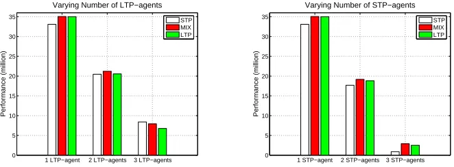
Given this background, five groups of experiments were con-ducted to examine the performance of each kind of agent in various situations. The number of MIX-agent, LTP-agent and STP-agent were: in setting A (1, 1, 1), in setting B (1, 2, 1), in setting C (1, 1, 2), in setting D (1, 1, 3), and in setting E (1, 3, 1). In each case, the remaining agents are the dummy agent provided by the organiser. The average revenue of each kind of agent in each experiment is
then plotted (see figure 7).
Now, in figure 7a, the results for setting A, B and E are pre-sented.10 Here from A to B to E, we increase the number of LTP-agents and decrease the number of dummy LTP-agents. In setting A, MIX- and LTP-agents perform significantly better than the STP-agent,11but we cannot differentiate statistically which is better be-tween MIX- and LTP-agents. In setting B, we cannot differentiate statistically which agent is better among these three type of agents. In setting E, the STP-agent is significantly better than the LTP-agent and MIX-LTP-agent is slightly better than the LTP-LTP-agent. But we cannot differentiate statistically which agent is better between STP-and MIX-agents. From these three experiments, we can conclude that with an increasing number of LTP-agents, the performance of the STP- and MIX-agents are getting better, while that of the LTP-agent is relatively worse. This is because more LTP-agents are request-ing components for the far future, leavrequest-ing more spare production capacities for the suppliers in the near future. Thus the component price for the near future will drop which means the agents that pur-chase many more components in the near future will benefit from this price and thus have a low cost.
Similarly, in figure 7b, the result for settings A, C and D are presented. Here from A to C to D, we increase the number of STP-agents and decrease the number of dummy STP-agents. In settings A
10The performance for the dummy agents are not shown in the figure
since they are much worse than these three type of agents and incor-porating them would make it difficult to see the difference among the three.
11In this case and in the statistics below, significance is computed
1 LTP−agent 2 LTP−agents 3 LTP−agents 0
5 10 15 20 25 30 35
Performance (million)
Varying Number of LTP−agents
STP MIX LTP
1 STP−agent 2 STP−agents 3 STP−agents 0
5 10 15 20 25 30 35
Performance (million)
Varying Number of STP−agents
STP MIX LTP
[image:8.612.136.467.54.176.2](a) Experimental results for settings A, B and E. (b) Experimental results for settings A, C and D. Figure 7: Comparison of performance in various settings.
and C, MIX- and LTP-agents are significantly better than the STP-agent. But we cannot differentiate statistically which agent is better between MIX- and LTP-agent. This is because there are only two agents that purchase components for far away which is not likely to cause the price increase of the components in the far future. But for the STP-agent, there are some dummy agents which order compo-nents for a due date in the next several days, thus more competition in the near future leads to an the increase in the component price and higher overall procurement costs. In setting D, we obtain the same result as in setting C, but with a much smaller pvalue of the Student’s t-test. This means the performance of STP-agents are actually getting worse when there are more agents like itself. How-ever, in all the cases we investigated, the MIX-agent is the most stable one as it performs consistently in the presence of various numbers of STP- and LTP-agents. Overall, it obtains the highest average performance (17.82) and the lowest variance (11.68).
Moreover, as more agents use the same broad strategy of sens-ing the market and ordersens-ing intelligently for the near and far future, the performance of all the agents are negatively affected, (i.e., the performance of all the agents is getting worse from experiment A through B to E, and from A through C to D). This happens because as the agents within the game become increasingly homogeneous, there is greater competition for components at a given time (be-cause there are several agents ordering components for broadly the same due date for the far future), and thus the suppliers have less spare capacity, and component costs increase.
4.
CONCLUSIONS
This paper provides a number of insights into building agents for supply chain management applications. Specifically, it details the design, implementation and evaluation of SouthamptonSCM; an agent that successfully participated in the 2005 TAC SCM. This agent employs fuzzy reasoning to determine how to set prices and uses a mixed component procurement strategy that balances long and short term orders. Through analysing an actual competition game from the 2005 final we found that this strategy enables Southamp-tonSCM to buy more components at lower prices than the other most successful agents in the game. In a series of controlled exper-iment, where we varied the number of short-term and long-term-planning agents in the game, we found that the mixed procurement strategy was the most stable in all the cases that we considered.
Now, as well as being successful with the TAC SCM competi-tion, several aspects of our agent design and strategy are applicable in a wider context. Firstly, the general structure of the component agent is to employ a mixed strategy where orders in the far fu-ture cover the minimum baseline quantities needed in low demand
markets, whilst orders in the near future handle current changing demand. This mixture of baseline and opportunistic purchasing be-haviour is a common strategy in this domain and the technology we develop for achieving this can be readily transferred. Second, we believe our pricing model technology will also be useful in real SCM applications where just undercutting competitors’ prices can significantly improve profitability. Specifically, to apply our model in other domains, the designers of the rule base would need to adapt the fuzzy rules to reflect the factors that are most relevant. Now we believe that customer demand and inventory level are highly likely to be critical factors for almost all cases and thus these rules can remain unaltered. By using different rule bases, different factors can easily be incorporated (as we did here, in order to handle the additional need to reduce inventory towards the end of the game).
Our future work in this area focuses on the component agent. We would like to improve it so that it can adapt the quantity for far fu-ture and near fufu-ture procurement automatically between the rounds of the games according to the procurement behaviours employed by the opponents. This can be achieved based on our controlled exper-iment results, where if there are more LTP-agents in the game, the agent will adapt its behaviour to the direction of STP-agent. Sim-ilarly, if there are more STP-agents, the best response is to change the buying behaviour to the direction of the LTP-agent. This knowl-edge of opponnets’ behaviour can be obtained from the game his-tory and thus this adaptation can be used in repeated games within the same participants.
5.
REFERENCES
[1] J. Collins, R. Arunachalam, et al. The supply chain management game for the 2005 trading agent competition. Technical Report
CMU-ISRI-04-139, School of Computer Science, Carnegie Mellon University, December 2004.
[2] M. He, H. F. Leung, and N. R. Jennings. A fuzzy logic based bidding strategy for autonomous agents in continuous double auctions.IEEE Transactions on Knowledge and Data Engineering, 15(6):1345–1363, 2003.
[3] M. He, A. Rogers, E. David, and N. R. Jennings. Designing and evaluating an adaptive trading agent for supply chain management applications. InProc. IJCAI Workshop on Trading Agent Design and Analysis, pages 35–42, Edinburgh, Scotland, 2005.
[4] K. Kumar. Technology for supporting supply-chain management.
Comms of the ACM, 44(6):58–61, 2001.
[5] D. Pardoe and P. Stone. Predictive planning for supply chain management.Proc. International conference on automated planning and scheduling, to appear.
[6] M. Sugeno. An introductory survey of fuzzy control.Information Sciences, 36:59–83, 1985.