An approach for constructing parsimonious generalized Gaussian kernel regression models

Neurocomputing 62 (2004) 441–457

An approach for constructing parsimonious

generalized Gaussian kernel regression models

X.X. Wang

, S. Chen

, D.J. Brown

a_{Intelligent Systems and Diagnostics Group, Department of Electronic and Computer Engineering,} University of Portsmouth, Anglesea Building, Anglesea Road, Portsmouth PO1 3DJ, UK

b_{School of Electronics and Computer Science, University of Southampton, Highfield,} Southampton SO17 1BJ, UK

Received 25 March 2004

Abstract

The paper proposes a novel construction algorithm for generalized Gaussian kernel regression models. Each kernel regressor in the generalized Gaussian kernel regression model has an individual diagonal covariance matrix, which is determined by maximizing the correlation between the training data and the regressor using a repeated guided random search based on boosting optimization. The standard orthogonal least squares algorithm is then used to select a sparse generalized kernel regression model from the resulting full regression matrix. Experimental results involving two real data sets demonstrate the effectiveness of the proposed regression modeling approach.

r2004 Elsevier B.V. All rights reserved.

Keywords:Neural networks; Regression; Orthogonal least squares; Correlation; Boosting

1. Introduction

A fundamental principle in practical nonlinear data modeling is the parsimonious principle of ensuring the smallest possible model that explains the training data. www.elsevier.com/locate/neucom

0925-2312/$ - see front matterr2004 Elsevier B.V. All rights reserved. doi:10.1016/j.neucom.2004.06.003

_{Corresponding author.}

Forward selection using the orthogonal least squares (OLS) algorithm [3–6,8]is a simple and efficient construction method that is capable of producing parsimonious linear-in-the-weights nonlinear models with excellent generalization performance. Alternatively, the state-of-art sparse kernel modeling techniques, such as the support vector machine and relevant vector machine [19,21–23], have been gaining popularity in data modeling applications. These existing sparse regression modeling techniques typically place the kernel centers or mean vectors at the training input data and use a fixed common kernel variance for all the regressor kernels. The value of this common kernel variance obviously has a critical influence on the sparsity and generalization capability of the resulting model, and it has to be determined via some sort of cross validation. For example, in [8] a genetic algorithm is applied to determine the appropriate common kernel variance through optimizing the model generalization performance.

In this paper, we consider a generalized Gaussian kernel model, in which each kernel regressor has an individually tuned diagonal covariance matrix. Such a generalized kernel regression model has the potential of improving modeling capability and producing sparser final models, compared with the standard approach of single fixed common variance. The difficult issue is then how to determine these kernel covariance matrices. Since the correlation function between a kernel regressor and the training data defines the ‘‘similarity’’ between the regressor and the training data, it can be used to ‘‘shape’’ the regressor by adjusting the associated kernel covariance matrix in order to maximize the absolute value of this correlation function. A weighted optimization algorithm, which has its root from boosting

[9,16,18], is considered to perform the associated optimization task. This weighted optimization algorithm is a guided random search method and the solution obtained may depend on the initial choice of population. To provide a robust optimization and guarantee stable solutions regardless of the initial choice of population, the algorithm is augmented into a repeated weighted optimization method.

The determination of kernel covariance matrices essentially provides the full bank of regressors or the full regression matrix, and this allows the application of the standard OLS algorithm[3,4]to select a parsimonious subset model. The outline of the paper is as follows. Section 2 gives the generalized Gaussian kernel regression model to be considered. Section 3 derives the correlation criterion to be used for determining the kernel covariance matrices and presents a repeated boosting search optimization algorithm for performing the corresponding optimization tasks. Section 4 briefly summarizes the standard OLS algorithm used to select a sparse kernel regression model, while Section 5 describes our modeling experiments. Finally, Section 6 offers our conclusions.

2. Generalized Gaussian kernel regression model

Consider a general discrete stochastic nonlinear system represented by

where uk and yk are the system input and output variables, respectively, nu and ny are positive integers representing the known lags in uk and yk; respectively, the observation noise ek is uncorrelated with zero mean, xk¼ ½y_k1 y_kny uk1 uknu

T _{denotes the system input vector with a known}

dimension n¼nyþnu; fsð Þ is a priori unknown system mapping, and h is an unknown parameter vector associated with the appropriate, but yet to be determined, model structure. The system model (1) is to be identified from an N-sample system observational data setDN ¼ fxk;y_kgN_k¼1;using some suitable functions which can approximatef_sð Þwith arbitrary accuracy.

We will model the unknown dynamical process (1) by using the following generalized Gaussian kernel regression model

y_k¼y^_kþek¼

XN

i¼1

yig_iðxkÞ þek ð2Þ

where y^_k denotes the model output given the input xk;yi are the model weight parameters, andg_ið Þare the kernel regressors. We allow the regressor function to be chosen as the general Gaussian functiong_iðxÞ ¼Gðx;xi;SiÞwith

Gðx;xi;SiÞ ¼exp1₂ðxxiÞTSi1ðxxiÞ ð3Þ

where the kernel covariance matrix takes the form ofSi¼diagfs2i;1;. . .;s2i;ng:As is in a standard kernel regression model, the kernel mean vectors are placed at the training input data points. If all the diagonal covariance matrices are set to the identical form of diagfs2_{;. . .;s}2_{g;we arrive at the standard Gaussian kernel model.}

The kernel model (2) over the training setDNcan be written in the matrix form as

y¼Ghþe ð4Þ

by defining

y¼ ½y₁ y₂ y_NT ð5Þ

h¼ ½y1 y2 yNT ð6Þ

e¼ ½e1 e2 eNT ð7Þ

G¼ ½g₁ g₂ g_N ð8Þ

g_i¼ ½g_iðx1Þgiðx2Þ giðxNÞT; 1pipN: ð9Þ The objective of sparse modeling is to construct a subset model consisting of Ns ð5NÞsignificant regressors only from the full set of regressors defined in (9).

3. Determination of the full regression matrix

the discussion by defining the least squares cost or mean square error (MSE) associated with anm-term model as

Sm¼ 1

N

XN

k¼1

ðyky^kÞ2 ð10Þ

where for the notational simplicity the same notationy^_kis also used for representing

them-term model output. ObviouslyS0¼yTy¼ kyk2:

3.1. Correlation criterion

The correlation between a regressorg_i and the training data is defined by

CðSiÞ ¼

yTg_i ffiffiffiffiffiffiffiffi yT_y

p ffiffiffiffiffiffiffiffiffi gT

igi

p ð11Þ

This correlation is a function of the regressor’s kernel covariance matrix. We propose to use this correlation function as the optimization criterion to determine the regressor’s kernel covariance matrix. Specifically, we should chooseSi so that jCðSiÞjis maximized. Why this is a good strategy to specify the pool of regressors can easily be explained. Assuming that g_i is selected to form a one-term model, the associated reduction in the MSE value can be shown to be

DS¼S0S1¼

ðyTg_iÞ2

gT_ig_i ð12Þ

which can be rewritten as

DS¼ ðyTyÞ ðy

T_g

iÞ2 ðyT_yÞðgT

igiÞ

¼ kyk2jCðSiÞj2 ð13Þ

Sincekyk2 is a constant, maximizingjCðSiÞj leads to a maximum reduction in the MSE value.

Having chosen the optimization criterion, we now turn our attention to optimization algorithm. We propose a repeated guided random search method to perform the associated optimization tasks. This algorithm adopts ideas from boosting[9,16,18].

3.2. Weighted optimization algorithm

is generated by a weighted combination of SðiÞ_{;1pipp: Because this weighted}

combination is a convex combination, the point Sðpþ1Þ _{is always within the}

convex hull defined by the p values. A (p+2)th point is then generated as the mirror image ofSðpþ1Þ_{;with respect to S}best_{;along the direction defined by S}best Sðpþ1Þ_{:The best ofS}ðpþ1Þ_andSðpþ2Þ_{then replacesS}worst_{:The process is repeated until}

it converges.

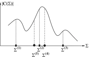
A simple illustration is depicted in Fig. 1 for a one-dimensional case, where there are p=3 points, Sð1Þ_{; S}ð2Þ _{and S}ð3Þ_{; and S}best_¼Sð2Þ _{and S}worst_¼Sð3Þ_{: The}

4th value Sð4Þ _{is a weighted combination of S}ð1Þ_{; S}ð2Þ _{and S}ð3Þ_{; and S}ð5Þ _{is the}

mirror image of Sð4Þ _{with respect to S}ð2Þ_{:As S}ð4Þ _{is better than S}ð5Þ _{in this case, it}

replaces Sð3Þ_{: Clearly, how the weighted combination is performed is critical.}

The weightings for SðiÞ_{;1pipp; should reflect the ‘‘goodness’’ of S}ðiÞ_{; and}

the process should be capable of self-learning or adapting these weightings. This is exactly the basic idea of boosting [9,16,18]. Specifically, by combining the AdaBoost algorithm of [9] with the above-mentioned simple search strategy, we arrive at the weighted optimization algorithm. Given the training data DN and for fitting the lth regressor’s covariance matrix, the algorithm is summarized as follows.

Initialization: Set iteration indext=0, give theprandomly chosen initial values for

Sl;Sðl1ÞðtÞ;S

ð2Þ

l ðtÞ;. . .;S

ðpÞ

l ðtÞ; with the associated weightings d

ðtÞ

i ¼1=p for 1pipp; and specify a small positive valuexfor terminating the search.

Step1:Boosting

1. Calculate the loss of each point in the population, namely

costi¼1 jCðSlðiÞðtÞÞj; 1pipp

2. Find

Sbest_l ðtÞ ¼arg minfcosti; 1pippg and

Sworst_l ðtÞ ¼arg maxfcosti; 1pippg

|C(Σ)|

Σ Σ(1) (2) (3)

Σ(5)ΣΣ(4) Σ

3. Normalize the loss

lossi¼ costi

Pp j¼1costj

; 1pipp

4. Compute a weighting factorb_t according to

Zt ¼

Xp

i¼1

dð_itÞlossi; bt¼

Z_t

1Z_t

5. Update the weighting vector

dð_itþ1Þ¼ d ðtÞ

i blosst i forbtp1;

dð_itÞb1lossi

t forbt41;

(

1pipp

6. Normalize the weighting vector

dð_itþ1Þ¼ d ðtþ1Þ

i

Pp j¼1d

ðtþ1Þ

j

; 1pipp

Step2:Parameter updating

1. Construct the (p+1)th point using the formula

Sð_lpþ1ÞðtÞ ¼X p

i¼1

dð_itþ1ÞSð_liÞðtÞ

2. Construct the (p+2)th point using the formula

Sð_lpþ2ÞðtÞ ¼Sbest_l ðtÞ þ ðSbest_l ðtÞ Sð_lpþ1ÞðtÞÞ

3. Choose a better point (smaller loss value) fromSð_lpþ1ÞðtÞandSð_lpþ2ÞðtÞto replace

Sworst_l ðtÞ;which will inherit the weighting dvalue fromSworst_l ðtÞ:1

Sett¼tþ1 and repeat from Step 1 until kSð_lpþ1ÞðtÞ S_lðpþ1Þðt1Þkox

Then choose thelth regressor covariance matrix asSl¼Sbestl ðtÞ:

The algorithmic parameter that needs to be set appropriately is the population size

p. The population size depends on the dimension ofSand the objective function to

be optimized. Generally, an appropriate value ofphas to be found empirically. This is very similar to for example the choice of population size in the genetic algorithm.

1

EachSð_liÞ; 1pipp;has an associated weighting valuedi:WhenSðlpþ1ÞorS ðpþ2Þ

l replacesSworstl ;it will keep the weighting value ofSworst

3.3. Repeated weighted optimization algorithm

The above weighted optimization algorithm performs a guided random search and the solution obtained may depend on the initial choice of population. To derive a robust algorithm that guarantees a global optimal solution, one may incorporate the full idea of the scatter search [10–12] with this weighted optimization algorithm. However, to avoid an overly complicated algorithm, we simply augment the algorithm into the following repeated weighted optimization algorithm. The aim is not to guarantee a global optimal solution. Rather it is to make sure that the algorithm will arrive at similar solutions regardless of the initial choices of population.

Initialization: Give a positive integer number M for controlling the

maximum repeating times, and choose a small positive numberx1 for terminating

the search.

First generation: Randomly choose the p number of the initial population

Sð_l1Þ;. . .;Sð_lpÞ; and call the weighted optimization algorithm to obtain a solution

Sbest_l :

Repeat loop: Fori=1:M

SetSð_l1Þ¼Sbest_l ;and randomly generate the otherp1 pointsSð_liÞ for 2pipp: Call the weighted optimization algorithm to obtain a solutionSbest_l :

IfkSð_l1ÞSbest_l kox1

Exit loop; End if

End for

Choose thelth regressor’s covariance matrix asSl¼Sbestl :

The important algorithmic parameter that need to be chosen appropriately is the termination criterionx1:Basically,x1 determines whether the solutions obtained in

different runs of the weighted optimization are closely enough to be regarded as the same solution. If a too smallx1is chosen, the loop may keep going for long time. To

safeguard against this, we also specify the maximum repeating times M. Again, appropriate values forMandx1 depends on the dimension ofSand how hard the

objective function to be optimized. Also the choice ofp has some influence on the choice of M and x1: Generally, these algorithmic parameters have to be found

empirically.

4. OLS algorithm for subset model selection

Once the full regression matrixGhas been designed, the standard OLS algorithm

[3,4]can be used to select a subset model. Let an orthogonal decomposition of the regression matrix be

where

A¼

1 a1;2 a1;N 0 1 .. . ...

.. . . . . . . .

aN1;N

0 0 1

2 6 6 6 6 6 4 3 7 7 7 7 7 5

ð15Þ

and

U¼ ½u₁ u₂ u_N ð16Þ

with orthogonal columns that satisfyuT_iu_j¼0;ifiaj:The regression model (4) can alternatively be expressed as

y¼Uwþe ð17Þ

where the orthogonal weight vectorw¼ ½w1 w2 wNTsatisfy the triangular system

Ah¼w: ð18Þ

KnowingAandw;h can readily be solved from (18). For the orthogonal regression model (17), the MSE

SN ¼

1

N e

T

e ð19Þ

can be expressed as

SN ¼

1

N y

T_y 1

N

XN

i¼1

/T_i/iw2i: ð20Þ

Thus the MSE for thel-term subset model can be expressed recursively as

Sl¼Sl1

1

N/

T

l/lw2l: ð21Þ

At thelth stage of regression, thelth term is selected to maximize the error reduction criterion[3,4]

DSl¼ 1

N /

T

l/lw2l: ð22Þ

The forward selection procedure is terminated at theNsth stage if

SNsoz ð23Þ

is satisfied, where the small positive scalarzis a chosen tolerance. This produces a parsimonious model containingNs significant regressors.

the MSE over the validation data set stops improving. Instead of using the pure least squares cost (20), it is also worth pointing out that other criteria can alternatively be adopted for the orthogonal forward selection, and these include regularization, optimal experimental design, and leave-one-out cross validation criterion[5,6].

5. Modeling examples

Two real-data sets were used to demonstrate the effectiveness of the proposed sparse model construction algorithm. The population sizep, the maximum repeating timesMand the termination criterionx1were chosen empirically to ensure that the

OLS subset selection procedure could produce consistent final models with the same levels of modeling accuracy and model sparsity for repeating runs.

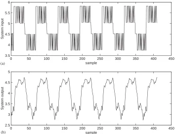
Example 1. This example constructed a model representing the relationship between the fuel rackposition (inputuk) and the engine speed (outputyk) for a Leyland TL11 turbocharged, direct injection diesel engine operated at low engine speed. Detailed system description and experimental setup can be found in[1]. The data set, depicted inFig. 2, contained 410 samples. The first 210 data points were used in training and

0 50 100 150 200 250 300 350 400 450 3.5

4 4.5 5 5.5 6

sample

System input

0 50 100 150 200 250 300 350 400 450 2.5

3 3.5 4 4.5 5

sample

System output

(a)

(b)

the last 200 points in model validation. The previous study[1]has shown that this data set can be modeled adequately as

y_k¼f_sðxkÞ þek ð24Þ

withf_sð Þ describing the unknown underlying system and the system input vector defining by

xk¼ ½yk1 uk1 uk2T ð25Þ

The previous results[5,6]have shown that when fitting a Gaussian kernel model with a single common variance, s2_{¼1:69 is the optimal value for this kernel}

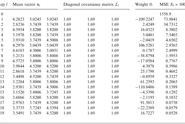
variance. Since every training input data points were considered as a candidate regressor’s center, there were 210 regressors for the full Gaussian kernel model. With the tolerance level set toz¼5:5104;the OLS algorithm selected a 19-term subset model from the full regression model, and the resulting subset model is listed in

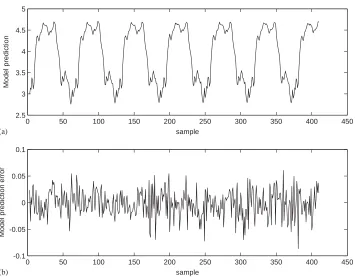
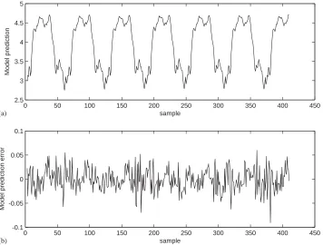
Table 1. The MSE values of the resulting model were 5:28104for the training set and 6:72104 _{for the validation set, respectively. Fig. 3shows the corresponding}

model predictiony^_kand the model prediction errorek¼yky^k:

The proposed sparse model construction algorithm was then applied to construct a generalized Gaussian kernel model. The algorithmic parameters of the repeated

Table 1

Subset model generated for the engine data set by the OLS algorithm with a Gaussian kernel model of a single common variance

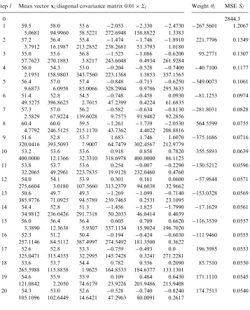
Stepl Mean vectorxl Diagonal covariance matrixSl Weightyl MSESl100

0 1558.9

weighted optimization for kernel covariance fitting were chosen to bep= 37,M= 60 and x1 ¼0:0002: Using the same tolerance level of z¼5:5104; the OLS

algorithm selected a 11-term subset model from the full generalized Gaussian kernel model, and the obtained model is listed inTable 2. The MSE values of this model were 5:09104 _{over the training set and 5:1910}4 _{over the validation set,}

respectively. The model prediction and prediction error generated by this model are illustrated inFig. 4.

Example 2. This example constructed a model for the gas furnace data set (Series J in[2]). The data set, illustrated inFig. 5, contained 296 pairs of input–output points, where the inputukwas the coded input gas feed rate and the outputy_krepresented CO2 concentration from the gas furnace. All the 296 data points were used in

training, with the model input vector defined by

xk¼ ½yk1 yk2 yk3 uk1 uk2 uk3T: ð26Þ

For this data set, the previous experiments have found out that it was difficult for the existing state-of-art kernel regression techniques to fit a Gaussian kernel regression model using a common kernel variance [6]. Various existing state-of-art kernel regression techniques were then used in[6]to fit a thin-plate-spline regression model 0 50 100 150 200 250 300 350 400 450 2.5

3 3.5 4 4.5 5

sample

Model prediction

0 50 100 150 200 250 300 350 400 450 -0.1

-0.05 0 0.05 0.1

sample

Model prediction error

(a)

(b)

Table 2

Subset model generated for the engine data set by the OLS algorithm with a generalized Gaussian kernel model

Stepl Mean vectorxl Diagonal covariance matrixSl Weightyl MSESl100

0 1558.9

1 4.6030 5.8006 5.8006 4.6610 23.2494 18.7487 52.9824 0.9292 2 4.5114 5.8006 5.8006 4.2126 22.5550 18.0605 53.9543 0.1655 3 4.4579 5.0245 5.8006 2.7926 14.5527 33.8069 74.9670 0.1202 4 4.4503 5.0051 5.8006 3.5534 360.546 12.8974 74.5696 0.1134 5 3.2284 5.8006 5.8006 311.554 12.6886 7.5157 246.1931 0.1129 6 4.6183 5.0051 5.8006 4.8006 48.6543 12.6258 96.1724 0.1007 7 3.6637 5.8006 5.8006 190.214 12.6563 7.5715 245.7579 0.0898 8 4.3510 5.0245 5.0245 2.8708 6.8213 253.1952 13.8707 0.0813 9 3.1062 4.5394 3.7245 400.00 400.00 400.000 2.5807 0.0642 10 4.3663 5.0439 5.8200 2.2056 40.4580 75.2890 50.1908 0.0592 11 3.9233 3.7439 4.5200 2.0241 327.7485 263.2715 4.3783 0.0509

The kernel covariance matrices are determined by maximizing the correlation criterion using the repeated weighted optimization algorithm.

0 50 100 150 200 250 300 350 400 450 -0.1

-0.05 0 0.05 0.1

sample

Model prediction error

0 50 100 150 200 250 300 350 400 450 2.5

3 3.5 4 4.5 5

sample

Model prediction

(b) (a)

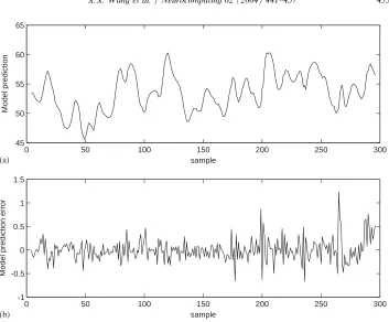
for this data set and the best result obtained required at least 30 model terms to achieve a modeling accuracy ofz¼0:054:

The proposed sparse model algorithm was employed to construct a generalized Gaussian kernel model for this data set. The kernel covariance matrices were first determined using the repeated weighted optimization with the following algorithmic parameters: p=100, M=60 and x1¼0:0001: With the modeling accuracy of z¼

0:054; the OLS algorithm constructed a 20-term subset model from the full generalized Gaussian kernel model, as is listed inTable 3. The model prediction and prediction error generated by this model are shown inFig. 6.

6. Conclusions

A novel construction algorithm has been developed for the generalized Gaussian kernel model. Each kernel regressor in the pool of candidate regressors has an individual diagonal covariance matrix, which is determined by maximizing the absolute value of the correlation between the regressor and the training data using a repeated weighted search optimization. The standard orthogonal least squares 0 50 100 150 200 250 300 45

50 55 60 65

sample

System Output

0 50 100 150 200 250 300 -3

-2 -1 0 1 2 3

sample

System Input

(a)

(b)

Table 3

Subset model generated for the gas furnace data set by the OLS algorithm with a generalized Gaussian kernel model

Stepl Mean vectorxl/diagonal covariance matrix 0:01Sl Weightyl MSESl

0 2844.3

1 59.5 58.0 55.6 2.053 2.330 2.4730 267.5601 1.2067 5.0681 94.9960 58.5221 272.6948 158.8822 1.3383

2 57.2 56.4 55.4 1.474 1.746 1.8910 221.7796 0.1549 3.7912 16.1987 213.2852 238.2681 51.3793 1.0180

3 55.0 55.6 56.8 1.525 1.086 0.6200 95.2771 0.1307 57.7623 270.1883 3.8217 243.6048 0.4934 261.9284

4 56.0 54.3 53.0 0.204 0.528 0.7400 40.7100 0.1177 2.1951 158.9803 343.7560 223.1368 1.3853 357.1565

5 56.4 57.0 57.4 0.848 0.713 0.6250 349.0073 0.1061 9.6873 6.0958 85.0066 328.2904 0.9786 295.3635

6 51.4 52.8 54.5 0.748 0.458 0.0930 81.1253 0.0974 49.5275 396.8625 2.7015 47.2399 0.4224 61.6835

7 57.3 57.0 56.2 0.582 0.634 0.8130 281.8031 0.0828 2.5829 67.9224 139.6028 9.7573 91.9482 92.2856

8 60.4 60.0 59.5 1.261 1.739 2.0530 564.5599 0.0755 4.7792 246.5125 215.1170 43.7362 4.4022 208.8816

9 51.6 52.8 53.7 1.683 1.746 1.6070 375.1686 0.0716 320.0416 393.5093 7.9007 64.7479 302.4567 212.9779

10 53.2 53.6 53.6 0.918 0.858 0.7820 355.5893 0.0639 400.0000 12.1366 32.3310 318.6978 400.0000 86.1125

11 53.8 53.7 53.6 0.254 0.007 0.2290 150.5212 0.0596 32.2065 49.2961 223.7835 19.9128 232.0460 0.4760

12 54.0 54.1 53.9 0.301 0.161 0.0600 57.9844 0.0571 275.6604 3.0180 107.5660 313.2379 94.6038 32.9662

13 50.6 49.7 49.3 1.269 1.099 0.7140 153.0328 0.0569 385.9776 71.0925 94.5789 239.7465 0.2531 23.1095

14 54.4 52.8 51.3 1.456 1.825 1.7990 17.1629 0.0561 34.9812 236.0426 291.7318 50.2033 46.0414 0.4039

15 56.0 56.4 56.4 0.605 0.709 0.6620 116.3539 0.0557 3.3890 12.3638 5.9307 337.1134 15.9024 196.7020

16 52.3 51.2 50.4 0.194 0.424 0.6030 111.9460 0.0555 257.1146 84.5112 387.4997 274.5492 181.3500 0.3622

17 52.6 52.8 53.3 0.759 0.493 0.0 196.3985 0.0553 325.0471 315.4355 32.2995 145.7428 0.3241 271.2281

18 53.6 53.7 54.4 0.782 0.556 0.2090 85.7510 0.0550 265.5988 115.8858 1.9625 164.8533 184.6377 133.1301

19 54.6 55.9 55.9 0.109 0.484 0.6430 171.1110 0.0545 121.0842 2.2050 74.6179 23.9226 201.9486 215.9408

20 54.3 53.0 52.6 0.528 0.740 0.8240 174.7513 0.0540 105.1096 102.6449 14.6421 47.2963 80.0091 0.2617

algorithm is then applied to select a parsimonious model from the full regression matrix. Compared with the existing kernel regression modeling approaches which adopt a single common kernel variance for all the regressors, the proposed method has the advantages of improving modeling capability and producing sparser models. These advantages have been demonstrated by the experimental results involving two real data sets.

References

[1] S.A. Billings, S. Chen, R.J. Backhouse, The identification of linear and non-linear models of a turbocharged automotive diesel engine, Mech. Syst. Signal Process. 3 (2) (1989) 123–142.

[2] G.E.P. Box, G.M. Jenkins, Time Series Analysis, Forecasting and Control, Holden-Day Inc., San Francisco, 1976.

[3] S. Chen, S.A. Billings, W. Luo, Orthogonal least squares methods and their application to non-linear system identification, Int. J. Control 50 (5) (1989) 1873–1896.

[4] S. Chen, C.F.N. Cowan, P.M. Grant, Orthogonal least squares learning algorithm for radial basis function networks, IEEE Trans. Neural Networks 2 (2) (1991) 302–309.

0 50 100 150 200 250 300 -1

-0.5 0 0.5 1 1.5

sample

Model prediction error

0 50 100 150 200 250 300 45

50 55 60 65

sample

Model prediction

(a)

(b)

[5] S. Chen, X. Hong, C.J. Harris, Sparse kernel regression modelling using combined locally regularized orthogonal least squares and D-optimality experimental design, IEEE Trans. Automat. Control 48 (6) (2003) 1029–1036.

[6] S. Chen, X. Hong, C.J. Harris, P.M. Sharkey, Sparse modelling using orthogonal forward regression with PRESS statistic and regularization, IEEE Trans. Syst. Man Cybernet. Part B 34 (2) (2004) 898–911.

[7] S. Chen, B.L. Luk, Adaptive simulated annealing for optimization in signal processing applications, Signal Process 79 (1) (1999) 117–128.

[8] S. Chen, Y. Wu, B.L. Luk, Combined genetic algorithm optimisation and regularised orthogonal least squares learning for radial basis function networks, IEEE Trans. Neural Networks 10 (5) (1999) 1239–1243.

[9] Y. Freund, R.E. Schapire, A decision-theoretic generalization of on-line learning and an application to boosting, J. Comput. Syst. Sci. 55 (1) (1997) 119–139.

[10] F. Glover, A template for scatter search and path relinking, in: J.-K. Hao, E. Lutton, E. Ronald, M. Schoenauer, D. Snyers (Eds.), Artificial Evolution, Lecture Notes in Computer Science, vol. 1363, Springer, Berlin, 1998, pp. 13–54.

[11] F. Glover, Scatter search and path relinking, in: D. Corne, M. Dorigo, F. Glover (Eds.), New Ideas in Optimization, McGraw-Hill, New York, 1999, pp. 297–316.

[12] F. Glover, M. Laguna, R. Marti, Scatter search and path relinking: foundations and advanced designs, 2002, submitted for publication.

[13] D.E. Goldberg, Genetic Algorithms in Search, Optimization and Machine Learning, Addison-Wesley, Reading, MA, 1989.

[14] L. Ingber, Simulated annealing: practice versus theory, Math. Comput. Model. 18 (11) (1993) 29–57. [15] K.F. Man, K.S. Tang, S. Kwong, Genetic Algorithms: Concepts and Design, Springer, London,

1998.

[16] R. Meir, G. Ra¨tsch, An introduction to boosting and leveraging, in: S. Mendelson, A. Smola (Eds.), Advanced Lectures in Machine Learning, Springer, Berlin, 2003, pp. 119–184.

[17] R.H. Myers, Classical and Modern Regression with Applications, second ed., PWS-KENT, Boston, 1990.

[18] R.E. Schapire, The strength of weaklearnability, Mach. Learn. 5 (2) (1990) 197–227.

[19] B. Schlkopf, A.J. Smola, Learning with Kernels: Support Vector Machines, Regularization, Optimization, and Beyond, MIT Press, Cambridge, MA, 2002.

[20] M. Stone, Cross validation choice and assessment of statistical predictions, J. R. Stat. Soc. Ser. B 36 (1974) 117–147.

[21] M.E. Tipping, Sparse Bayesian learning and the relevance vector machine, J. Mach. Learn. Res. 1 (2001) 211–244.

[22] V. Vapnik, The Nature of Statistical Learning Theory, Springer, New York, 1995.

[23] V. Vapnik, S. Golowich, A. Smola, Support vector method for function approximation, regression estimation, and signal processing, in: M.C. Mozer, M.I. Jordan, T. Petsche (Eds.), Advances in Neural Information Processing Systems, vol. 9, MIT Press, Cambridge, MA, 1997, pp. 281–287.

Sheng Chenobtained a B.Eng. degree in control engineering from the East China Petroleum Institute, Dongying, China, in 1982, and a Ph.D. degree in control engineering from the City University at London in 1986. He joined the School of Electronics and Computer Science at the University of Southampton, UK, in September 1999. He previously held research and academic appointments at the Universities of Sheffield, Edinburgh and Portsmouth, UK. Dr. Chen is a Senior Member of IEEE. His recent research works include adaptive nonlinear signal processing, modeling and identification of nonlinear systems, machine learning and neural networkresearch, finite-precision digital controller design, evolu-tionary computation methods and optimization. He has published over 200 research papers.