White Rose Research Online URL for this paper: http://eprints.whiterose.ac.uk/99558/
Version: Accepted Version
Article:
Cantarella, GE and Watling, DP orcid.org/0000-0002-6193-9121 (2016) A General
Stochastic Process for Day-to-Day Dynamic Traffic Assignment: Formulation, Asymptotic Behaviour, and Stability Analysis. Transportation Research Part B: Methodological, 92 (Part A). pp. 3-21. ISSN 0191-2615
https://doi.org/10.1016/j.trb.2016.05.005
© 2016, Elsevier. Licensed under the Creative Commons Attribution-NonCommercial-NoDerivatives 4.0 International http://creativecommons.org/licenses/by-nc-nd/4.0/
[email protected] https://eprints.whiterose.ac.uk/ Reuse
Items deposited in White Rose Research Online are protected by copyright, with all rights reserved unless indicated otherwise. They may be downloaded and/or printed for private study, or other acts as permitted by national copyright laws. The publisher or other rights holders may allow further reproduction and re-use of the full text version. This is indicated by the licence information on the White Rose Research Online record for the item.
Takedown
If you consider content in White Rose Research Online to be in breach of UK law, please notify us by
Giulio E. Cantarella, University of Salerno David P. Watling, University of Leeds
Abstract This paper presents a general modelling approach to day-to-day dynamic assignment to a congested network through discrete-time stochastic and deterministic process models including an explicit modelling of users habit as a part of route choice behaviour, through an exponential smoothing filter, and of their memory of network conditions on past days, through a moving average or an exponentially smoothing filter. An asymptotic analysis of the mean process is carried out to provide a better insight. Results of such analyses are also used for deriving conditions, about values of the system parameters, assuring that the mean process is dissipative and/or converges to some kind of attractor. Numerical small examples are also provided in order to illustrate the theoretical results obtained.
1.
Introduction
The development, since the 1970s, of efficient computational methods for implementing network equilibrium models has arguably had one of the most significant impacts of academic research on transport planning practice. In many countries, such methods are an embedded element of procedures for cost-benefit analysis of proposed schemes, and are used widely for operational planning of traffic measures. With this class of approach now extended to consider multiple classes of users, within-day dynamic traffic interactions, unreliability and heterogeneity/mis-perception of users, their potential applicability is wider than it has ever been. Such facts are important to appreciate when proposing any approach that may be viewed as an alternative to the network equilibrium philosophy. Many large transport investments have been justified on the basis of equilibrium
predictions and so there is a political price in practitioners moving to any new method
Academic researchers can help considerably in this process by better understanding the linkages between what might appear to be apparently diverse methods, and in particular by understanding the connection of any alternative approaches to network equilibrium. The objective, for example, could be to better understand the cases in which network equilibrium may be justified as an approximation to some real-world situation, and those cases in which it may potentially give misleading results. The present paper is motivated by exactly this desire to better understand the connections between approaches, and to understand where network equilibrium is a useful notion in this context. This includes the possibility, in some cases, that we calculate equilibrium in exactly the same way as we do at present, but the meaning or conceptualisation of the computed state is different, and suggests additional or alternative ways to utilise the computed state.
The focus of the present paper will be on what have become known as day-to-day dynamic models of route choice, focusing on among other elements how users adapt their route
decisions over repeated trips The term day-to-day dynamic is useful to distinguish these
approaches from within-day dynamic models these latter focusing on issues such as time-dependent OD demand rates, the spatial and temporal interactions of traffic flows, the influence on users time-dependent choice of route and possibly departure time, and the possibility for users to make en route diversions during a journey. In order to focus our discussion, we do not consider within-day dynamic issues in the present paper, though we note that there are several papers that consider the combination of day-to-day and within-day dynamics Cascetta & Cantarella, 1991; Balijepalli & Watling, 2005; Liu et al, 2006; Friesz et al, 2011, and note that it is possible to transfer many of the arguments of the kind used here admittedly at the price of far greater complexity to the combined case. We
note that the term day-to-day dynamic is intended, therefore, to be indicative of the kind
of process being considered, but it need not be that these models are representing a real, continuous sequence of complete days. In this respect it is good to have in mind the following suggestion of an epoch-to-epoch dynamic model where
epochs can have either a chronological interpretation as successive reference
periods of similar characteristics e.g. the a.m. peak period of successive working days
or they can be defined as fictitious moments in which users acquire awareness of path
attributes and make their choices Cascetta, 1989
associated with traditional equilibrium models of transport systems, in the sense that point equilibria may emerge, under certain assumptions, as the convergent limits of such processes under some long-term steady conditions. DPs also allow transitions to be
examined especially when some shock or designed change occurs He & Liu, 2012. A recent review and synthesis of DP models in discrete and continuous time may be found in Cantarella & Watling 2015; in this paper no comparison is carried out with DPs in continuous time and/or based on Wardrop approach to route choice behaviour for a recent paper see Guo et al., 2015, since results obtained with these models can hardly transferred to the kind of models discussed in this paper.
SPs are more naturally associated with modelling the variability that is seen to occur in real-life systems, even under relatively stable operating conditions; they are thus able to represent both dynamic transitions and steady-state fluctuations. A review of SP models is provided in Watling & Cantarella 2014. The two types of approach draw on quite different mathematical disciplines, DPs emerging from non-linear dynamical system theory typically interested in mappings over continuous state spaces, whereas SPs arising originally from the study of probability theory and Markov chains over discrete state space.
Although some numerical evidence relating DPs and SPs exists e.g. Cantarella & Cascetta, 1995; Watling, 1996, relatively little general, theoretical evidence exists concerning their relation for general traffic networks. The exceptions to this are the works of Davis & Nihan 1993 and Hazelton & Watling 2004, both of whom developed asymptotic approximation results for SPs, as demands and capacities grow in tandem. In the present
paper we develop a natural relation between DPs and SPs which emerges from viewing
DPs as a joint process in the statistical moments of the corresponding SP. This work is inspired by the general asymptotic theory mentioned above, and the series of two-link examples recently studied in Watling & Cantarella 2013. We shall here extend the work presented in Watling & Cantarella 2013 in several ways, particularly focusing on the development of the mean of a SP as a DP, as well as other results in literature.
The models presented and discussed in this paper extend our previous theoretical work on discrete-time stochastic and deterministic process models into a general modelling approach to day-to-day dynamic assignment so as to: a relate to general traffic networks (not just two-link networks); b include an inertia/habit effect modelled through an exponential smoothing filter; and c incorporate learning models with finite or infinite memory, bridging moving average and exponentially smoothed approaches.
The theoretical approximation of an SP model is first derived as a DP in the vector of flow means. Analysing the resulting DP, conditions are established to ensure uniqueness of the equilibrium, and to ensure its local asymptotic stability, conditions for the system being dissipative are also stated. Numerical examples are provided in order to motivate the work, to illustrate the theoretical results obtained, and to explore the generality of the asymptotic large demand/large capacity approximation, even in cases where demand
The paper is organised as follows. Section 2 presents basic notations and briefly reviews SUE models; then section 3 discusses some simple but effective approaches to modelling dynamic learning and choice behaviour and analyses resulting Deterministic Process models.Section 4 describes the proposed SP model and some solution approaches as well as an asymptotic approximation to the mean of this process. Finally, in sections 5 and 6 we discuss the main findings and identify several potential future research directions.
2.
Basic notations, definitions and equations in SUE models
In this section we will briefly review the basic notations and definitions adopted, as well as fixed-point models for stochastic user equilibrium assignment Cantarella, 1997.
Our starting is that demand is segregated into multiple classes, each class containing users moving on the same origin-destination OD movement and in the same user category i.e. with the same behavioural parameters1. Let
nCL be the number of user classes;
ni be the number of acyclic or elementary routes available for users of class i;
n = i ni be the total number of routes available across all user classes2;
di > 0 be the demand flow for user class i, assumed integer and greater than zero;
d be the demand flow vector of dimension nCL;
D[i] = di Ini be a diagonal matrix of dimensions ni ni, with entries on the main diagonal equal to di;
p[i] 0 and 1Tp[i] = 1 be the route fraction vector of dimension ni for user class i;
x[i] = dip[i] 0 and 1Tx[i] = di be the route flow vector of dimension ni for user class i;
D be a n n block diagonal matrix, with each block given by D[i];
p be the route fraction block vector of dimension n, with each block given by p[i];
x = Dp 0 be the route flow block vector of dimension n, with each block given by x[i];
w[i] be the route cost vector of dimension ni for user class i;
w be the route cost block vector of dimension n, with each block given by w[i];
nLINK be the number of links;
c be the link cost vector of dimension nLINK;
f be the link flow vector of dimension nLINK;
fb be the link base flow vector of dimension nLINK, link flows not depending from modelled
user route choice behaviour;
B be the nLINK n link-route incidence matrix, with entries equal to 1 or 0 depending on whether a link is part of the given route. Each class is assumed connected by at least two routes, since the demand flow of any user class with only one available route induces further link flows that can be directly added to the base link flowvector fb,.
The link flows are given by:
1 For readers unfamiliar with such notation, it is suggested that on a first reading it makes sense to suppose
there is a single user category and so classes refer only to origin-destination pairs, and then on a second reading to consider the generalisation to multiple user categories, since conceptually there is little difference.
2 It is worth noting that according to the above notations the collection of acyclic routes available for travel, across all classes are indexed n, in such a way that the ni routes corresponding to class i have indices
f = B x + fb
We shall suppose the route travel costs w are sum of a term linear-additive in the generic
link travel costs:
w = BTc + wo
where possibly of another term including specific or non-additive route costs, wo.
Congestion on the nLINK links of the network is modelled through travel cost functions: c = cf
In most cases the link travel cost actually depends on the flow capacity ratio, rather than on the flow value itself.
Then the link travel cost-flow functions imply corresponding route travel cost-flow functions such that the route travel costs when the route flows are x are given by:
wx = BTcBx + fb + wo
In our subsequent analysis this implied relationship above between route costs and route flows, will often be used rather than the underlying relationship between link costs and link flows.
The route choice fractions p result from the user route choice behaviour and can be expressed as a function of the route disutilities by applying any model derived from the Random Utility Theory, such as Logit, C-Logit Probit Gammit :
p[i] = p[i]z[i] i nCL
p = pz
where in this case:
z[i] = w[i]x is the route disutility vector of dimension ni for user class i;
z = wx is the route disutility block vector of dimension n, with each block given by z[i]. The stochastic user equilibrium assignment searches for mutually consistent flows and costs, assuming that a RUM is used to described the route choice behaviour. It can be expressed by fixed-point models with respect to route or arc flows or costs, such as:
xSUE = DpwxSUE 2.1
Existence of solution is guaranteed if both the cost function and the route choice model are continuous and the network is connected. Uniqueness is guaranteed under the commonly adopted conditions of positive definiteness of the Jacobian of cost function,
Jw = x wx, and the negative semi-definiteness of the choice probability function Jacobian,
Jp = zpz, the latter holding under mild assumptions Cantarella, 1997. Furthermore, as
discussed in Bifulco et al 2013 and in therein quoted references, the invertibility of the matrix I D Jp Jw is a weaker sufficient condition to guarantee uniqueness of the SUE
solution.
3.
Modelling learning and choice behaviour in DP models
The specification of a day-to-day dynamic process models for assignment requires the explicit modelling of
user habit: how users make a choice today, possibly repeating yesterday choice to avoid the effort needed to take a decision, or reconsidering it according to the forecasted level of service,
user learning and forecasting process: how users forecast the level of service that they will experience today, from experience and other sources of information.
In this section we will describe some simple approaches to address the two above issues sub-sections 3.1 and 3.2, which will allow us to specify and analyse a Stochastic Process SP model in the following section 4. In this section a Deterministic Process DP model is also analysed sub-section 3.3 to support comparison between two approaches to user learning and forecasting process and to approximate the mean process of the SP model. We suppose a learning process for users whereby the disutility zjt 1 of each route j forecasted at the end of travelling on day t 1 is used when making decisions for the following day t. This forecasted disutility is assumed to be the accumulated knowledge up to the end of day t 1, so generalising the notion of disutility introduced in the above section 2. Let
xt be the route flow block vector on day t;
zt be the forecasted route disutility block vector on day t.
3.1 Modelling the dynamic choice process
In the following, we specify how users make decisions based on learnt experiences modelled as in the following sub-section 3.2. Specifically, we assume:
A fixe proportion 0 < 1 of users reconsider their previous day s choice and those that do decide to reconsider then make choices in proportions according to a random utility model possibly then repeating the previous day s choice; and
The remaining users choose between the available routes in proportions equal to the
fraction of users that actually chose those routes on the previous day.
Under such a behavioural model, users of class i are now assumed to have two reasons for choosing any route j available for them: either they choose it out of habit, which a proportion xjt-1 /diof them do where xjt-1 is the number of users that actually chose route
j yesterday, and di is the class demand flow for class i, or their choice behaviour can be
modelled through a RUM, such as Logit, C-Logit Probit The proportion of users choosing for the first reason is 1 and for the second reason is . For those that do decide to reconsider their choice, then conditionally on the vector of disutilities zt 1at the end of day t 1, each user of class i chooses a route independently of one another, with choice proportions given by a random utility model, with the proportions of choosing a route j
collection of all such functions across the all the classes as: pzt 1 . Then we get an exponential smoothing filter ES:
xt = Dpz
t 1 + 1
xt 1 t 3.1 or xt = D
pz
t 1 + 1
D-1xt 1 t Equation 3.1 tries to model in simple but effective way user inertia to change and how much users are prone to review their habit; this simple model also allows us to develop the consideration about convergence and stability in sub-section 3.3. In more general approaches the proportion may itself be a function of some disutility reliability variables. For instance in approaches regarding ATIS equipped users may depend on the ATIS aggregate reliability, and thus may change over time. This issue is addressed by Bifulco and Simonelli 2005, Bifulco et al. 2007, 2009, 2011 through a modelling approach consistent with this paper. However, embedding this approach in a complete multi-user framework allowing for the kind of stability analysis carried out in sub-section 3.3 is still an open issue see also section 6.
In disaggregate approaches, a proportion is defined for each route separately depending on the difference between experienced and forecasted or ATIS provided costs. The use of probabilistic thresholds leads to route choice switching models. This approach is rather effective when only two routes are available between each O-D pair, since there is no need of any route choice model. Indeed, when more than two routes are available, a conditional route choice function should be applied to model route choice behaviour of users who decide to reconsider their yesterday choice.
3.2 Modelling the learning behaviour process
We have seen Cantarella, 2013, for further details, and Bifulco et al, 2014, for further models that in the case of DP models, an especially convenient form of specification of learning model is one in which the forecasted disutility at the end of a day say yesterday is a convex combination of the previous day s forecasted disutility and the present day s actual travel cost:
zt-1= wxt-1 + 1 zt 1 t = 1, 2, 3 3.2 where the memory weighting parameter satisfies 0 < 1, and where at t = 1, we suppose:
z0= wx0 for a given route flow vector x0. Under such a model, we may recursively apply the expressions above in order to relate the forecasted disutility on any day t to the complete history of travel costs and hence flows since the beginning of the process, leading to an exponential smoothing filter ES:
zt-1= wxt-1 +
k t-1 1 k-1wxt-k + 1 t 1 wx0 t .We note that from the viewpoint of representing real-world systems, the assumption of an
infinite learning model adopted in several previous studies of the deterministic process model was made due to the considerable mathematical simplicity it affords, being an approximation of real-world user behaviour see below for some numerical examples, rather than a belief that users never forget an experience, however old. It is therefore quite easy to justify an assumption of finite memory, and we shall adopt this in our stochastic process analysis in section 4. We shall, however, specify this model in order to capture the possibility at one extreme of mimicking as closely as possibly the infinite memory assumption commonly adopted in studies of deterministic process models.
Therefore, we shall use the relative weighting of actual travel costs as suggested by the -model above, but will truncate the past memory by only considering some pre-specified fixed number of previous days m. This means that at day t, we only start the summation at day t m + 1. In order that the truncated process retains the property of being a convex combination of the actual costs, we apply a scaling factor to ensure that the non-neglected weights sum to 1, leading to a convex moving average filter with normalised decreasing weights defined by one-parameter MA, m and for < 1 and m > 1 given by:
k = 1 k 1/1 1 m 0 k m with
k = 1 and ]0,1] or k = k-1 1 k m with 1 = / 1 1 m It is worth noting that condition = 1 and m > 1 yields to 1= 1 and k+1 = 0 k m,moreover for m = 1 it is assumed 1= 1. Since all these conditions lead to a ES1 filter, a
proper MA filter is only obtained with m > 1 and < 1 that is 1 < 1. If the weights k are
assumed strictly decreasing with respect to k, then1 > 1/m.
In this case after the initialization step see below, the forecasted disutilities are given by:
zt-1 = / 1 1 m wxt-1 +
k m k wxt kor zt-1 =
k m k wxt k t = m +1, m 3.3 or zt-1 = CMt-1 where CMt-1 is the m n memory matrix of costs with m columns given by the costs in the
m previous days, wxt k k m.
At the end of each day t-1 the current cost memory matrix CMt-2is updated by dropping last column, moving all others columns rightwards and putting wxt-1 as first column in
CMt-2. Initialization of CMt, say specification of CM0, may be carried out assuming that: all the m columns of 0 are equal to wx0 for any given route flow vector x0; the ES filter 3.2 is applied for m days to fill the m columns of matrix 0.
It is worth noting that as m goes to infinite we get the exponential smoothing filter described above by equation 3.2 with either of the above initialization approaches. Moreover as m goes to infinite,
1 = / 1 1 m > goes to ,
m = 1 m 1/1 1 m > 0 goes to 0.
Moreover, looking at equation 3.3, we can see that the weights given to actual travel experiences in the past depend only on the relative distance in time they are away from the present, i.e. the model MA, m is time-homogeneous.
3.3 Stability analysis through Deterministic process models
This subsection analyses whether the system described by the deterministic process model DP 3.1, 3.3 based on MA filter is dissipative with respect to the memory depth m
and the memory weighting parameter . A brief review of results concerning DP 3.1, 3.2 based on ES is also reported below for comparison s sake In all DP models discussed below fixed-points states given by xt = xt-1 = x* are equal to the SUE flow pattern x
SUE. Three cases will be discussed below depending on values of memory depth m and of memory weighting parameter , whichever is the value of habit parameter = 1 leading to particular cases. [Appendix 1 briefly review deterministic process models, say discrete-time discrete-time-homogeneous Markovian non-linear systems.]
We will first assume that the memory is large enough that other past days are considered beside yesterday but not all past days, say 1 < m < , and < 1, thus 1 > and m > 0. In
this case it is necessary to re-formulate DP 13.1, 3.3 to obtain a Markovian DP.
The system state at day t is described by a m-block vector, one block hxth = 1, ..., m 1 for each of the m days to be kept in memory. Thus: the first block 1xtcontains today s route flows, as in vector xt already introduced; the second block 2xt contains yesterday s route flows, say xt-1; and so on. Therefore, on each day t today s flowscontained in the first block 1xt are updated according to equation 3.1, then each of all the other blocks are
used to keep a memory of the previous days flows whilst the m-th day in the past is no
longer recorded According to this state definition today s state only depends on
yesterday s leading to the following Markovian DP
1xt = 1 1xt 1 + Dp
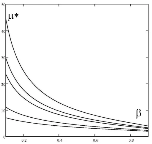
k ,m k wkxt 1 3.4 h+1xt = hxt-1 h = 1, ..., m 1 3.5 From the analysis reported in Appendix 2 it turns out that the system may not be dissipative, especially for high values of and low values of m. However, whichever is the value of , there always exists a large enough memory depth m* such that for any memory deeper than this value m* the system is dissipative from any starting state.Figure 1 Value m against need to obtain a value of m
less than: 0.1, 0.05, 0.01, 0.005, 0.001 from top to bottom.
This brief analysis shows that the DP systems based on MA filter for modelling learning process may not be dissipative, that is may not converge to any kind of attractor from some starting states at least as time goes to infinite. On the other hand, if the memory depth is large enough the system is always dissipative. A full stability and bifurcation analysis of this case is still an open issue, worth of further research effort.
On the other hand, if < 1 and the memory depth is so large that it may be considered infinite, no day is ever forgotten even though just a small weight is given to days far in the past, say m , then 1 and m 0. In this case MA filter 3.3 tends to the ES 3.2
filter whichever is the value of , and we get the general Markovian DP model recently discussed in detail in Cantarella 2013. The determinant of the Jacobian of such a model is 1 n1 nalways in the range ] 1, 1[, thus the system is always dissipative, that is it always converges to an attractor not necessarily a fixed-point from any starting state. In that paper an in-depth fixed-point stability and bifurcation analysis is carried out and further earlier references are also reported.
A special case is obtained if memory refers to yesterday only, m = 1, or = 1 then for MA filter 1 = m = 1, thus the MA , m = 1, the MA = 1, m and the ES = 1 filters give the same DP model:
xt = 1 xt 1+ Dpwxt 1 3.6 DP 3.6 is Markovian with Jacobian matrix J given by:
J = 1 I + G where G = DJp Jw
Since the determinant of J may be out of the range ] 1, 1[, the system may be not
dissipative, that is it may not converge to any kind of attractor. In this case even if there is a unique fixed-point x*, it may be an attractor from some starting states only but not from all, or it is not an attractor at all. An in-depth fixed-point stability and bifurcation analysis can easily be carried out noting that for each eigenvalue of matrix G an eigenvalue of matrix J is given by 1 + , being a special case of the case briefly discussed above.
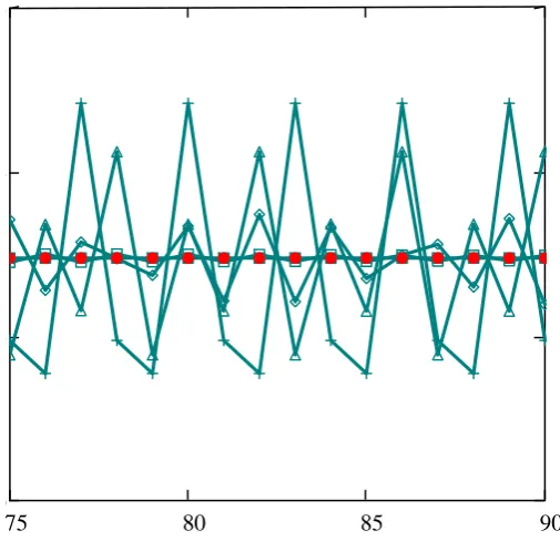
Figure 2 shows the evolution of a route flow from day 75 to day 90 basic data are in appendix 3 applying DP with MA with memory depth m or with ES. DP with MA and m = 6 is almost undistinguishable of DP with ES both reach a fixed-point attractor equal to the unique SUE. It can easily be seen that a short memory leads the system towards other kind of attractors than the unique fixed-point, which is not locally stable.
Figure 2. A route flow against day given by DP with MA m = 2, 3, 4, 5, 6, and with ES see also the text above.
It seems worth noting that all results presented above still hold if the DP model 3.1, 3.3 or 3.1, 3.2 are formulated with respect to link variables; this is always the case when route choice user behaviour is modelled through random utility models. On the other hand, if this behaviour is modeled according to Wardrop I principle, link- and route- based models are generally different see for instance Guo et al., 2015.
kk:= k0 kmax..
75 80 85 90
0 1000 2000 3000
[image:12.595.175.428.270.514.2]4.
A Stochastic Process model for day-to-day assignment
In conventional SUE models we are familiar with the idea of modelling randomness/heterogeneity in users perceptions of travel costs, and we also include here such a feature. Additionally we shall here suppose that the actual travel costs experienced are also randomly distributed. In the present paper we suppose that the only source of randomness in the actual travel costs is the randomness in flows. This is an extreme and unnecessarily restrictive assumption, and in practice there are likely to be many other unobserved sources of variation in the actual travel costs, e.g. due to weather, incidents, vehicle-mix. The model defined could be extended to represent such variations, either through postulating a probability distribution of elements of the parameters of the cost functions e.g. the capacities, and/or by assuming additional additive variation on the distribution of travel costs generated by variable flows and/or variable parameters i.e. this would be in addition to the flow-based variation captured in the postulated model. These are important factors to consider, yet in line with the rest of the paper we neglect them here in order to focus on the main thrust of the paper. For a discussion of some additional sources of variation that might be modelled using such processes, the interested reader is referred to Watling & Cantarella 2013, 2014.
Due to the several sources of uncertainty above mentioned we suppose that the number of user travelling on route j on day t as well as the corresponding route disutility are modelled as random variables, Xjt and Zjt respectively, whose realisations are denoted by
xjt and zjt. Thus, let
Z[i] be the route disutility vector of dimension ni for user class i;
Z be the route disutility block vector of dimension n, with each block given by Z[i];
X[i] = dip[i] 0 and 1TX[i] = di be the route flow vector of dimension ni for user class i;
X be the route flow block vector of dimension n, with each block given by X[i].
4.1 The overall SP model
The above assumptions combined with the dynamic choice process 3.1 and the MA filter 3.3 or the ES filter 3.2, lead to an m-dependent Markov process in discrete state space, whereby the conditional probability distribution of the state on any day t, as represented through the vector random variable Xt, is fully determined by the previously-realised values of the states {Xt k: k m}. The assumptions may be summarised as:
| {Xt k: k m}~ Multinomialdi , 1 /di + p[i]Zt 1
independently for each i = 1, 2, nCL for some vector of cost functions w., choice model p., demand vector d , memory length
m 1, normalised learning weights {1, 2 m}, reconsideration probability 0 < 1.
Actually, it will be more convenient, below, to capture this model by writing it entirely equivalently as:
Zt 1=
k ,m k wXt k 4.1= 1 /di + p[i]Zt 1 4.2
where Y is the vector of the composite route choice probabilities, including both habit and choice process, for user class i, with entries yi.
Some remarks about model 4.1-4.3:
the composite route choice probability for route i, yi., is a random variable since it is a function of random variables;
the composite route choice probability for route i, yi., depends on route costs or
disutilities, even though probability does not in more advanced models probability may also depend on costs and disutilities, see section 6 for further comments;
according to equations 4.2 and 4.3 the choice behaviour of any two users of the same class or of different classes are assumed independent conditional on the remembered past states; still in the unconditional distribution all users route choices may affect all the others through congestion, say the cost function introduced in the sub-section 2.1;
equation 4.1 needs to be properly initialized as described in the sub-section 3.2
As established first by Cascetta 1989, if the random utility model p. is such that a
non-zero probability is assigned to all feasible alternatives as satisfied by regular random utility models defined on an infinite support, then the process above has a unique stationary probability distribution to which it converges, regardless of the initial conditions, that is it is regular.
Model 4.1-4.3 may be solved through Monte Carlo techniques. At this aim it is useful noting that a Multinomial random variable is obtained by independently repeating n times a Categorical also called "generalized Bernoulli" random variable in the very same way that a Binomial is obtained by independently repeating n times a Bernoulli r. v..
On each day t first disutilities Z are updated through equation 4.1, and choice probabilities Y through equation 4.2. Then for each user class i the inverse distribution function method is applied di times to the categorical distribution defined by the choice probabilities, using a sample of di pseudo-random numbers uniformly distributed over [0,1]. This way, an unbiased estimate of the mean of the route flows X is obtained; the same approach allows us to estimate any other moment, such as variance, and the unique stationary distribution. This solution approach may be applied to real cases, provided that routes are explicitly enumerated. Solution methods not requiring such enumeration are still an open issue.
From standard properties of the Multinomial distribution the corresponding mean process is given by:
E[ | Zt 1, Xt 1] = di 1 /di + p[i]Zt 1 =
= E[ | Zt 1, Xt 1] = 1 + dip[i]Zt 1 i = 1, 2, nCL. 4.4 It should be noted that E[ | Zt 1, Xt 1] in the above equation is a random variable since it is a function of random variables Zt 1 and Xt 1. Collecting equations 4.4 together across all classes, and using the notation for writing the demands introduced in section 2.1, it then follows that:
Applying a statistical identity to equation 4 above then yields an expression for the unconditional mean process:
E[Xt] = E[E[Xt|Zt 1, Xt 1]] =
= 1 E[Xt 1]+ D E[pZt 1] 4.5 A stability analysis of the mean process 4.5 requires that it is put in a Markovian form to apply results from deterministic process theory see appendix 2 for details. The DP model described in section 3.3 is an approximation to the mean process 4.5. An analysis of the variance will be the topic of a future paper.
If the above assumptions are combined with the dynamic choice process 3.1 and the ES filter 3.2 we get a 1-dependent Markov process but in continuous state space of flows and forecasted costs, as discussed in Cantarella and Cascetta 1995.
4.2 Asymptotic analysis
An asymptotic analysis of the mean process is carried-out in the next sub-sections, by further developing and extending the asymptotic analyses presented in Watling & Cantarella 2013, which drew on earlier work of Davis & Nihan 1993 and Hazelton & Watling 2004. It may be worth stressing that the purpose of this analysis is exploiting relationships with DP models not providing a solution method for real cases.
In order to make some progress in analytically capturing the evolution of this process, the analysis is based on an asymptotic analysis whereby we examine the behaviour of the process as the demands are scaled by > 0,and so the scaled demands are denoted by d, and in particular the behaviour of the process as becomes large, but in a special sense.
Since simply scaling the demand alone would clearly change the nature of the demand/network being modelled, and so not give any meaningful results, what we analyse
is what happens when the demand is scaled for the purposes of modelling route choice
but the scaling is reversed when it is substituted in the congestion relationships. We might think of this process, intuitively, as one in which demands and link capacities are scaled in
tandem, if we are adopting travel cost functions whose actual argument is the ratio of flow
to capacity. Thus if the vector x = x1, x2 xn denotes the flows under a demand scaling
of on the n routes of the network as above, then wjx denotes the travel cost on route j
when the route flows are x for j n . Noting that reversing the scaling the route
flow vector would be 1x
we are thus motivated to consider functions of the form: wjx = wj 1x
where wi. is a function independent of that is the underlying true route cost functions,
as defined in section 2.1. We use wx = w1x, w2x wnxT and w 1x = w1
1x, w2 1x w
n 1xT to denote the corresponding vector mappings.
All the above presented equations 4.1-4.5 can easily be re-written taking into account the scaling factor as:
Zt 1=
k m k wXt k 4.6 | Zt 1, Xt 1 ~ Multinomial di , 4.8
independently for each i nCL where notation highlights that the left hand side of equation 4.8 is slightly different from in equation 4.3 since it depends on scale parameter .
The corresponding mean process is given by:
E[ | Zt 1, Xt 1] = 1
+ dip[i]Z
t 1 i nCL. 4.9 E[Xt| Zt 1, Xt 1] = 1 Xt 1 + D pZt 1.
E[Xt] = E[E[Xt|Zt 1, Xt 1]] =
= 1 E[Xt 1]+ D E[pZt 1]. 4.10
After Cascetta 1989 the SP model 4.6, 7, 8 is regular. Furthermore, Davis & Nihan 1993 studied a wide class of stochastic process models, and showed that, as demand D in tandem with the network capacities, so the stationary distribution converges to
a multivariate normal distribution with mean equal to the conventional Stochastic User Equilibrium SUE solution.
The process we shall analyse is an extension of that considered by Hazelton & Watling 2004; their process is exactly ours for the case = 1. Like them we use Davis Nihan s result to develop an asymptotic approximation to moments of the stationary distribution of the process, based only on knowledge of the SUE solution and other input data to the traffic assignment process. Watling & Cantarella 2013 further extended this work for the case of uncongested two-route networks and for congested two-route networks with = 1, deriving expressions to describe the dynamics of the process only in terms of its means, variances and covariances. The body of work above has been the motivation for our present analysis. In particular we shall aim to extend the analysis of Watling & Cantarella 2013 to the case of general networks for a general value of 0 < 1. However, differently from the goals of these works, we shall focus on a process in which only the first moment, the mean, is used to approximate the evolution of the process, with a
particular goal to explore the relationship to equivalent deterministic process models which neglect variability.
In order to do so we make the following distributional approximations, following Hazelton & Watling 2004, where assuming w. and p. to be continuously differentiable:
wX = wxSUE + 1 Jw X xSUE + Op 0.5
pZ = pwxSUE + Jp Z wxSUE + Op 0.5
where
xSUE is the assumed unique SUE solution satisfying: xSUE = DpwxSUE, consistent with
defintion in section 2;
Jw = xwx = xSUE and Jp = zpz = wxSUE are respectively the Jacobian matrix of w.
evaluated at xSUE and the Jacobian matrix of p. evaluated at wxSUE.
of the random variable X as a linear transformation, given by the first order Taylor series approximation about the SUE solution.
From equation 4.10 we may obtain as proved in appendix 4 that: 1 I DJp Jw * = 1 I DJp Jw xSUE + O 0.5 .
where in stationarity * = t = t 1 = t 2 t m with t = E[Xt].
Now, as discussed in Bifulco et al 2013, the invertibility of the matrix I D Jp Jw is a
condition that may be adopted for assuming uniqueness of the SUE solution it is weaker than the commonly adopted conditions of positive definiteness of the Jacobian of cost function and the negative semi-definiteness of the choice probability function Jacobian. Thus, under the assumption that I DJp Jw 1 exists, and since > 0, we obtain:
1 * = 1xSUE + 1I DJp Jw 1 O 0.5 .
This generalises the model and the result in Hazelton & Watling 2004 to include habit modelling, say 0 < 1; indeed the model in Hazelton & Watling 2004 turns out to be a
special case where no kind of habit occurs, say = 1.
It implies that for large we have a justification to approximate 1 * by 1 xSUE, since *
and xSUE both grow with . The DP models 3.1, 3.3 and 3.1, 3.2 discussed in section 3.3
are an approximation to the asymptotic mean process above described.
4.3 Some numerical examples
This section reports the results of some numerical examples of the asymptotic behaviour of the SP model 4.6, 7, 8 comparing it with the DP model 3.1, 3. At this aim, it is useful to restate the model 4.6, 7, 8 as the following equivalent model with a slightly different definition of X as highlighted by notation X:
Zt 1=
k m k wXt k 4.11= 1 /di + p[i]Zt 1 4.12
| Zt 1, Xt 1 ~ 1/ Multinomial di, 4.13 independently for each i nCL where ri = di is the numbers of users given scale factor and demand flow di for each user class i. It is worth noting that this way equations 4.11 and 4.12 are equal to equations 4.1 and 4.2 respectively.
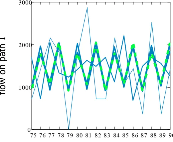
Figures 3 and 4 cfr Figure 2 show the evolution of a route flow from day 75 to day 90, for
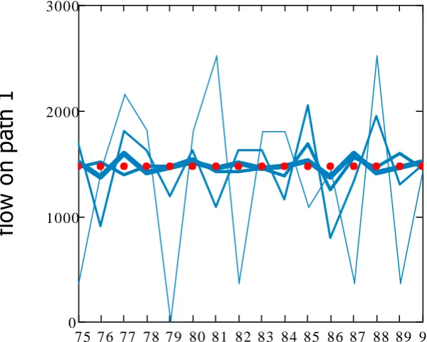
m = 3 and 5 respectively, as a results of SP model 4.11, 12, 13 with r = 10, 100, 1000, 10000 users3 and of the corresponding DP model 3.1, 3. The SP model has been solved through the Monte Carlo techniques already described. As expected from the above asymptotic analysis, results with the SP model with 10000 users are very close to those with the DP model. As the memory depth m increases from 3 to 5 the observed fluctuations become smaller for high numbers of users. Figure 5 cfr Figure 2 shows the evolution of a route flow from day 75 to day 90, for m = , that is with ES, as a results of SP
model 4.11, 12, 13 with r = 10, 100, 1000, 10000 users and of the corresponding DP model 3.1, 3. The reported results are consistent with those in Figures 3 and 4.
Figure 3. A route flow
against day with MA
and m = 3 given by
SP with10, 100, 1000, 10000 users thin to thick line, or DP dashed line as in Figure 2 .
75 76 77 78 79 80 81 82 83 84 85 86 87 88 89 90 0
1000 2000 3000
day
fl
o
w
o
n
p
a
th
1
75 76 77 78 79 80 81 82 83 84 85 86 87 88 89 90 0
1000 2000 3000
day
fl
o
w
o
n
p
a
th
[image:18.595.148.450.138.386.2]Figure 4. A route flow against day with MA and m = 5 given by SP with10, 100, 1000, 10000 users thin to thick line ,
or DP dashed line as in Figure 2 .
Figure 5. A route flow against day with ES given by SP with10, 100, 1000, 10000 users thin to thick line
or DP dotted line as in Figure 2 .
75 76 77 78 79 80 81 82 83 84 85 86 87 88 89 90 0
1000 2000 3000
day
fl
o
w
o
n
p
a
th
5.
Discussion
In the paper we have presented several technical results concerning stochastic process models, but in the midst of the technical details it can be easy to miss the key implications of the work. In this section we aim to draw out these implications.
Result 1: Asymptotic Mean Process Dynamics
(a)Asymptotically, as demands/capacities grow, in the stochastic process model the mean flows t depend only on {t k: k m}, and not on anything else in the previous
history of the process such as variances, covariances, etc. in previous days.
(b)Asymptotically, dependence oft on {t k: k m} is linear and can be expressed
through knowledge of only: the SUE solution, the choice probability Jacobian evaluated at SUE, the cost function Jacobian evaluated at SUE, the value of , the values of m and {k:
k m} and the demand vector d. Significantly, these are all input parameters,
orin the case of the SUE solutionsomething that can be readily derived from the input parameters without regard to the system dynamics.
To our knowledge, these result are not explicitly stated, and not in this way, in any previous papers, and anyway no previous paper showed the technical results for a case including inertia effects through . It holds for a general network and for multiple classes.
It is important to appreciate that Result 1 holds for any model of learning weights based on the previous m days, as long as the weights sum to one. It is not necessary that the learning weights decay with time, for example. We could have a learning process, for example, where users put a weight of zero on the previous 4 days and a weight of one on the experience 5 days ago as might occur, for example, in a model in which days are weekdays, and a user travelling on Fridays only learns from previous Fridays. It is also not necessary that the learning weights give rise to stable behaviour in the deterministic system above; still our dynamic equations hold for other types of system.
It is also important that Result 1 holds under a range of assumptions for the cost functions, cost function parameters, choice probability functions, choice probability function parameters, and value of . This will mean that it holds to describe processes that are very different in nature, with very different kinds of trajectory.
It should be remarked that Result 1 makes some distributional assumptions concerning the form of the cost functions and the choice probability functions, and their relation to the demand multiplier. We also assume a unique SUE. It seems we are making some restrictions, therefore, and so it be interesting to make further exploration of Result 1a in terms of what happens beyond these restrictions, e.g. with asymmetric cost functions and multiple SUE building on Watling, 1996.
Result 2: Asymptotic Result on Equilibrium of Mean Process and SUE
Asymptotically, the equilibrium of the mean process in Result 1 is an SUE, under certain conditions on the Jacobian of cost functions evaluated at SUE, the choice probability Jacobian
evaluated at SUE, and the demand vector, but not on the behavioural parameters and {k:
k m}.
This establishes that asymptotically, the point equilibria of the mean process are invariant to the behavioural parameters and {k: k m}. This corresponds to results known
for deterministic process models Cantarella & Cascetta, 1995.
Result 3: Asymptotic Result on Equilibrium of Mean Process
The nature of the approximate mean process, namely whether it is dissipative and/or whether it converges to a stable fixed point, is determined by , {k: k m}, and the Jacobian of the mean process evaluated at SUE.
In contrast to Result 2, this result establishes that the behavioural parameters affect the nature of the approximate mean process, but that we can anticipate this nature from knowing the behavioural parameters. Again, this corresponds to what is already known for deterministic process models Cantarella & Cascetta, 1995.
However, to balance these results we should also mention the following result:
Result 4: Asymptotically the variance of the process depends on more than the mean
It is not true that in general:Asymptotically as demands/capacities grow, in the stochastic process model the variance of the process at time tdepends only on {t k: k m}, and
not on anything else in the previous history of the process such as variances, covariances etc. in previous days.
In order to prove this negative result we may use a counter-example, for which we can refer to the analysis of two-link networks in Watling and Cantarella 2013. This negative result is important for addressing a relatively common mis-perception that modelling
6.
Conclusions and Research Perspectives
In this paper we have sought to integrate and extend various previous works concerning stability of deterministic processes and the analysis of stochastic processes. We have presented a generic stochastic process model for a general multi-class network, including notions of user habit, learning and choice, and have analysed this model theoretically by developing an asymptotic approximation for the mean process of such a model. We have shown how this approximating mean process relates to SUE. We have then used the tools of deterministic dynamical systems to analyse the mean process, and have shown how the nature of the learning process can be used to anticipate the nature of the mean process, including whether it is dissipative, converges to a stable fixed point, etc.
Even if the presented models and results are stated with respect to route costs, disutilities and flows, it seems worth noting that they hold as well with respect to link variables. Generally this is not the case for day-to-day dynamic models based on Wardrop route choice behaviour.
While the present paper has been wholly theoretical in nature, we believe that there is important future research in analysing such systems through Monte Carlo simulations of the process, as in the small numerical examples described at the end of sections 4 and 3. In doing so, insights may be obtained that would enrich and add to the theoretical insights provided here.
In particular, apart from open issues already mentioned above, linking to the Results we highlighted in section 5, we would suggest that interesting investigations would be to:
explore the impact on the process trajectory of the cost function parameters, choice model parameters and , and relate the findings to Result 1a;
explore analytically or numerically the transient time for the mean process to reach SUE from given starting conditions, as a function of ;
explore the impact of changing parameters to increase the variance of the process and
to see its consequential impact on the mean process, by changing the number of users
e.g. not large, or in cases with multiple SUE, or if the system is near-periodic, or the effect of the learning weights;
explore the impact of parameters, such as and , differentiated by user class;
re-examine Result 1a and extend results in sub-section 3.3 in the light of the various kinds of learning processes suggested by Horowitz 1984;
re-examine Result 1a and extend results in sub-section 3.3 in the light of of habit
models where changes over time depending on aggregate or disaggregate
difference between forecasted and experienced disutilities as proposed in some papers on continuous-time DP models;
illustrate and further explore Result 2 using the tests above;
illustrate and explore both stable and unstable cases, and relate to Result 3;
explore the strength of the dependence of the process on previous variance/
autocorrelations, and the extent to which knowledge of the mean is almost sufficient
Calibration of SP models is still open issue, see Parry & Hazelton 2013, and Shao et al. 2014 for some approaches to this problem.
Acknowledgements – Authors greatly appreciated the comments and suggestions received from
References
Balijepalli, N.C. and Watling, D.P. 2005. Doubly Dynamic Equilibrium Approximation Model for Dynamic Traffic Assignment.In: Transportation and Traffic Theory: Flow, Dynamics and Human Interaction ed.:H.Mahmassani, Elsevier, Oxford, UK, 741-760. Bifulco G.N., Cantarella G.E., Simonelli F., Velonà P. 2013. Equilibrium and day-to-day
stability in traffic networks under ATIS. In: Proceedings of the 3rd International Conference on Models and Technologies for Intelligent Transportation Systems, Dresden, pp 503 512.
Bifulco, G.N., Cantarella, G.E., Simonelli, F. 2014. Design of signal setting and advanced traveler information systems. J. of Intelligent Transportation Systems 181, 30-40. Cantarella G.E. 2013. Day-to-day dynamic models for Intelligent Transportation Systems
design and appraisal. Transportation Research Part C 29, 117 130.
Cantarella G.E & Cascetta E. 1995. Dynamic Process and Equilibrium in Transportation Networks: Towards a Unifying Theory. Transportation Science 29, 305-329.
Cantarella G.E. & Watling D.P. 2016. Modelling road traffic assignment as a day-to-day dynamic, deterministic process: a unified approach to discrete- and continuous-time models. In EURO J Transp Logist 2016 5:69 98.
Cantarella G.E., Gentile G., Velonà P. 2010. Uniqueness of Stochastic User Equilibrium. In Proceedings of 5th IMA conference on Mathematics in Transportation. London, UK, April 2010.
Cascetta E. & Cantarella G.E. 1991. A day-to-day and within-day dynamic stochastic assignment model. Transportation Research Part A 25, 277-291.
Davis G. & Nihan N. 1993. Large population approximations of a general stochastic traffic assignment model. Operations Research 41, 169-178.
Friesz, T.L., Kim, T., Kwon C., Rigdon, M.A. 2011. Approximate network loading and dual-time-scale dynamic user equilibrium. Transportation Research B 45, 176-207.
Guo Ren-Yong, Yang H., Huang Hai-Jun, Tan Z. 2015. Link-based day-to-day network traffic dynamics and equilibria. Transportation Research Part B 71, 248 260.
Hazelton M.L. & Watling D.P. 2004. Computation of equilibrium distributions of Markov traffic assignment models. Transportation Science 38, 331-342.
He X. & Liu H.X. 2012. Modeling the day-to-day traffic evolution process after an unexpected network disruption. Transportation Research Part B 46, 50 71.
Horowitz J.L. 1984.The stability of stochastic equilibrium in a two-link transportation network. Transportation Research Part B 18, 13-28.
Liu R., Van Vliet D. & Watling D. 2006. Microsimulation models incorporating both demand and supply side dynamics. Transportation Research Part A 40, 125-150.
Parry K. & Hazelton M. L. 2013. Bayesian inference for day-to-day dynamic traffic models. Transportation Research Part B 50, 104 115
Shao H., Lam W.H.K., Sumalee A. Chen Anthony 2014. Estimation of mean and covariance of peak hour origin destination demands from day-to-day traffic counts. Transportation Research Part B 68, 52 75.
Watling D.P. & Cantarella G.E 2013. Modelling sources of variation in transportation systems: Theoretical foundations of day-to-day dynamic models. Transportmetrica B 1, 3-32.