Simulation of the interaction between plasma turbulence and neutrals in linear devices

This is a repository copy of Simulation of the interaction between plasma turbulence and neutrals in linear devices.

White Rose Research Online URL for this paper: http://eprints.whiterose.ac.uk/106046/

Version: Accepted Version

Article:

Leddy, Jarrod, Willett, Hannah Victoria and Dudson, Benjamin Daniel

orcid.org/0000-0002-0094-4867 (2016) Simulation of the interaction between plasma turbulence and neutrals in linear devices. Nuclear Materials and Energy. ISSN 2352-1791 https://doi.org/10.1016/j.nme.2016.09.020

[email protected] https://eprints.whiterose.ac.uk/ Reuse

This article is distributed under the terms of the Creative Commons Attribution-NonCommercial-NoDerivs (CC BY-NC-ND) licence. This licence only allows you to download this work and share it with others as long as you credit the authors, but you can’t change the article in any way or use it commercially. More

information and the full terms of the licence here: https://creativecommons.org/licenses/

Takedown

If you consider content in White Rose Research Online to be in breach of UK law, please notify us by

Simulation of the interaction between plasma

turbulence and neutrals in linear devices

J.Leddy,

∗

B.Dudson, H.Willett

York Plasma Institute, University of York, Heslington UK YO105DD

Abstract

The interaction between plasma and neutrals within a tokamak dominates the be-haviour of the edge plasma, especially in the divertor region. This area is not quiescent, but has significant perturbations in the density and temperature due to turbulent fluctuations. Investigating the interaction between the neutrals and plasma is important for accurately simulating and understanding processes such as detachment in tokamaks. For simplicity, yet motivated by tokamak edge plasma, we simulate a linear plasma device and compare the sources and sinks due to ioni-sation, recombination, and charge exchange for cases with and without turbulence. Interestingly, the turbulence systematically strengthens the interaction, creating stronger sources and sinks for the plasma and neutrals. Not only does the strength of the interactions increase, but the location of these processes also changes. The recombination and charge exchange have relatively short mean free paths, so these processes occur on the scale of the eddy fluctuations, while the ionisation is mostly unaffected by the turbulence.

1 Introduction

In tokamaks heat is exhausted from the core into the edge plasma where it is then conducted along the magnetic field onto a very thin region on the divertor plates. Future fusion devices such as ITER will deposit so much power onto the divertor plates that, without intervention, severe melting could occur [1]. In addition to heat flux, particle flux through elastic collisions of molecules on the walls and divertor plays an important role in divertor conditions [2]; however, only particle flux is included here, and molecular flux is considered as potential future work. To decrease the heat flux, the plasma can be forced into a detached regime where much of the ther-mal and kinetic energy is radiated from the edge plasma and spread volumetrically. This occurs when the relatively low temperature plasma in the edge of a tokamak interacts strongly with neutrals near the divertor through charge exchange, ionisation, and recombination [3]. These atomic processes have cross-sections that are functions of the plasma temperature, density, and neutral density meaning that turbulence, which provides fluctuations in these quantities, will have a local effect on the plasma-neutral interactions. To explore these interactions qualitatively and quantitatively, simulations are performed of a linear plasma device. This provides a simple geometry in which to explore the effect of plasma turbulence on the plasma-neutral interaction.

Previous effort has been made in this area with statistically generated turbulence [4] and with two-dimensional SOL turbulence in TOKAM2D [5]; however, we seek to use self-consistent, 3D fluid turbulent simulations.

2 Physics models

In the tokamak divertor of existing devices, the plasma is usually collisional and can therefore be treated with a fluid approximation. The model used is based on one described by Simakov and Catto [6], but has been modified and put into finite volume form to conserve particle number and energy. This model, described in the next section, was then implemented in BOUT++ [7], which is a numerical framework for solving systems of differential equations in a range of geometries.

2.1 Plasma model

The model is electromagnetic, and evolves electron density ne, electron pressure pe, parallel ion momentum nv||i, plasma vorticity ω, and poloidal flux ψ. There is no separation between

background and fluctuations in this model, since we wish to study regions such as the tokamak edge where these are of similar magnitude. In the linear device to be simulated the magnetic field is constant in space and time, so magnetic drifts and curvature effects are omitted from this model.

∂ne

∂t =−∇ ·

neVE×B+nebvke

+∇ ·(D⊥∇⊥ne) +Sn−S (1)

3 2

∂pe

∂t =−∇ ·

3

2peVE×B+ 5 2pebv||e

−pe∇ ·VE×B+v||e∂||pe

+∇||

κe||∂||Te

+ 0.71∇||

Tej||

−0.71j||∂||Te+

ν nj 2 || (2) +∇ · 3

2D⊥Te∇⊥ne

+∇ ·(χ⊥ne∇⊥Te) +Sp −

2 3Q

∂ω

∂t =−∇ ·(ωVE×B) +∇||j||+∇ ·(µ⊥∇⊥ω) (3)

∂ ∂t

nev||i

=−∇ ·hnev||i

VE×B+bv||i i

−∂||pe+∇ ·

D⊥v||i∇⊥n

−F (4)

∂ ∂t

1

2βeψ−

me mi

j||

ne

=νj||

ne +∂||φ−

1

ne∂||pe−0.71∂||Te+ me mi

VE×B+bv||i

· ∇j||

ne (5)

with E×B drift given by:

VE×B =

b× ∇φ

B (6)

The vorticity is given by

ω =∇ ·

n

0

B2∇⊥φ

(7)

where the Boussinesq approximation is used, replacing ne with a constant n0 in the vorticity

equation. This expression is inverted to find the plasma potential φ. A cold-ion approximation is used such thatpi = 0. The plasma density source is given bySnand pressure (energy) source by Sp. The neutral interactions detailed in the next section provide sources for density S,

0 5 10 15 20 25 30 Electron temperature [eV]

10-20 10-19 10-18 10-17 10-16 10-15 10-14 10-13 10-12 Ra te < σv > [m 3s −

1]

Ionisation

Recombination (n =

m

)

Recombination (n =

m

)

Recombination (n =

m

)

Charge exchange

Figure 1. The cross-section rates for ionisation, recombination, and charge exchange are pre-calculated for hydrogen species as a function of the plasma temperature [15, 16].

pressure Q, and flux (friction) F. The density and thermal perpendicular diffusion coefficients are taken to be classical [8]. The parallel heat conductivity is defined as the Spitzer value,

κek = nv2thτe [9], where τe is the electron collision time. The resistivity, ν, is taken to be the

Spitzer resistivity [10]. Here we use the notation ∂||f =b· ∇f and ∇||f =∇ ·(bf).

2.2 Neutral model

A kinetic approach is often preferred for the description of neutral behaviour in the edge of tokamaks through codes such as EIRENE [11] because the neutral mean-free path can be larger than the machine size. This, however, is computationally expensive, and good qualitative agreement has been seen between simulation and experiment when fluid neutral models have been used with codes such as UEDGE [12]. For our simulations, a fluid-diffusive model is used such that the neutrals are treated as fluid parallel to the field lines so that parallel momentum is conserved in the plasma neutral interactions, with perpendicular motion dictated by diffusion [13, 14]. This system evolves neutral gas density nn, pressure pn and parallel velocity v||n:

∂nn

∂t =−∇ ·

nnbv||n+nnv⊥n

+S

∂ ∂t

nnv||n

=−∇ ·nnv||nbv||n+nnv||nv⊥n

−∂||pn+∇||

Dnnnn∂||v||n

+F

∂pn

∂t =−∇ ·

pnbv||n+pnv⊥n

−2

3pn∇ ·

bv||n

+∇ ·(Dnnnn∇⊥Tn) +

2 3Q

with

v⊥n =−Dnn

1

pn∇⊥pn

Figure 2. A simple schematic (left) of a linear device (Pilot-PSI in this case [18]) showing the basic geometry of the system. The magnetic field generated by the coils is roughly constant, pointing to the right. The plasma source on the left produces a plasma that streams along the field-lines until impacting the target on the right. The density contours along the plasma device are shown (right) for a turbulent case with the linear device dimensions indicated in meters.

important role in real devices, only radiative and 3-body recombination are considered in this model, which is essentially the same as that used in UEDGE [17]. The rates for these processes are given by

Rrc=n2

hσvirc Riz =nnnhσviiz Rcx=nnnhσvicx (8)

where n is the electron density, nn is the neutral density, hσvi is the rate coefficient for the given reaction (in m3

s−1

) which is a function of the local electron temperature (and density for recombination). These rate coefficients are calculated through a fit function of a database [15, 16], which are shown in figure 1. Given the rates in equation 8, the density source for the neutrals can be calculated:

S =Rrc−Riz (9)

The momentum transfer to the neutrals is given by

F =mivkiRrc−mivknRiz +mi

vki−vkn

Rcx (10)

Finally, the energy transfer to the neutrals is

Q= 3

2TeRrc− 3

2TnRiz + 3

2(Te−Tn)Rcx (11)

These sources for the neutrals are subtracted as sinks from the plasma equations as shown in section 2.1. Due to the cold-ion nature of the plasma model, there are two options in regards to charge exchange - either exclude it from thermal energy exchange or use the electron tem-perature in the energy transfer term. Since the plasmas of interest here (ie. tokamak edge and similar) has coupled ion and electron temperatures with significant energy loss from charge exchange, the latter method was chosen. A fully consistent model requires a hot ion treatment of the plasma, which will be explored in future work.

3 Linear device and turbulence

A linear device consists of a series of magnetic coils in a straight line configuration providing a constant magnetic field pointing along the device. A plasma source is then placed at one end, the plasma streams down the device, and hits a target at the far end (see figure 2). The linear device simulated here has a length of 1.2m and magnetic field of 0.15T. The plasma density

and power sources are set as spatial distributions that generate a Gaussian plasma profile with a standard deviation of 3.3cm, a peak temperature of 3eV, and a peak density of 1020

m3

at the source. The boundary conditions at the source end are zero gradient allowing outflow of plasma and neutrals, while sheath boundary conditions [19] are used at the target. Figure 2 shows a basic schematic of the simulated linear device along with a typical turbulent density contour. The plasma density is at a maximum near the source and decreases along the device towards the target plate. In the simulations presented here, a single species pure Deuterium plasma and neutral gas are assumed.

3.1 Turbulence in the linear device

The turbulence in the simulations of this linear device is electromagnetic in nature, driven by drift-waves that are a result of the radial pressure gradients from the localised plasma source. After evolving for 60000ω−1

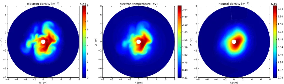
ci (roughly 1.25ms), the turbulence saturates. Figure 3 shows the

neutral and plasma density in the drift-plane (1m from the source for the plasma and at the target plate for the neutrals) at a single point in time. The neutral density at the target is highly correlated with the electron density due to the recycling, which is the dominant source for the neutrals. In real machines, gas leakage from the plasma source contributes to the ambient gas density and pressure, but in this simulation recycling and recombination are the only neutral sources. Interestingly, the peak plasma density can lie off-axis despite the density source having a maximum on axis, which is indicative of large perturbations over the background. The neutral density does not show fine scale features seen in the electron density for two reasons: firstly, the fluid model is diffusive, smoothing out features in the drift plane. In addition, the average lifetimes of the plasma and neutrals before recombination or ionisation (1/nhσvi ranging from 100µs to 0.1s), are larger than the turbulence correlation time (625ωci ≈ 13µs), meaning the neutrals essentially ‘see’ a time-averaged plasma. Using the instantaneous and local temperature to calculate the rate coefficients is justified because the longest ionisation and recombination processes complete in roughly 1µs [20], which is an order of magnitude below the turbulence correlation time. In this time, an average neutral particle moves roughly 0.1cm, which is an order of magnitude smaller than the turbulence correlation length. Neglecting the transport of excited states is therefore a reasonable assumption.

8 6 4 2 0 2 4 6 8 R [cm] 8 6 4 2 0 2 4 6 8 Z [cm]

electron density [m−3]

0 1 2 3 4 5 6 7 8 9 1e19

8 6 4 2 0 2 4 6 8 R [cm] 8 6 4 2 0 2 4 6 8 Z [cm]

electron temperature (eV)

0.21 0.48 0.75 1.02 1.29 1.56 1.83 2.10 2.37 2.64

8 6 4 2 0 2 4 6 8 R [cm] 8 6 4 2 0 2 4 6 8 Z [cm]

neutral density [m−3]

0.78 1.32 1.86 2.40 2.94 3.48 4.02 4.56 5.10 5.64 1e19

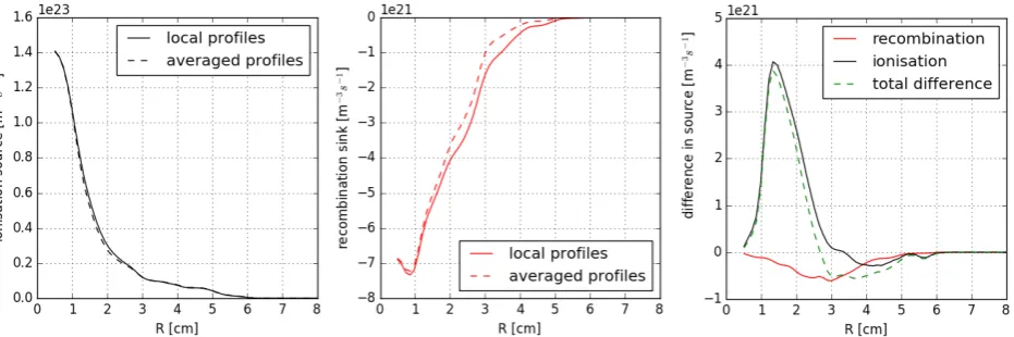
Figure 4. A comparison between average sources for turbulent (solid line) and non-turbulent (dashed line) cases. The resulting profiles for ionisation (left) and recombination (middle) are plotted. Finally, the difference between the turbulent and non-turbulent cases is shown (right).

4 Neutral-plasma interaction

In exploring the interaction between neutrals and plasma turbulence, two questions are answered. Firstly, is there a net effect of the turbulence on the sources and sinks for plasma density, momentum, and energy? Secondly, where are the interactions localised in the plasma column? These two questions are addressed in the following sections.

4.1 Net impact of plasma turbulence

By examining the data in two separate ways, the effect of the turbulence is isolated. First, the neutral density source is calculated (equation 9) using the local density and temperature and then averaged axially to produce radial profiles for the sources (turbulent ionisation source, for example: ¯St = nnnhσvi, where the bar over a variable indicates an axial average). This represents the average sources from turbulent profiles. Contrastingly, radial profiles for the sources can be obtained using axially averaged density and temperature profiles - this repre-sents the average source for a case where there is no turbulence (ionisation source, for example:

¯

S = ¯nnn¯ hσvi(Te)).

The results from these two cases are shown in figure 4. These radial profiles of the density sources are averaged over 10000ω−1

ci (roughly 16 fluctuation correlation times) and along the

axis of the device. The ionisation density source is increased with turbulence by 10% at maxi-mum. The recombination sink is also stronger with turbulence by a factor of 50% at maximaxi-mum. This can be seen clearly in the plot on the right in figure 4. The interaction of the neutrals with the local turbulent fluctuations consistently gives rise to stronger sources and sinks than the equivalent averaged profiles would. This consistent strengthening of the interaction appears to be universal due to the nonlinear dependence of the sources on the plasma density and temperature.

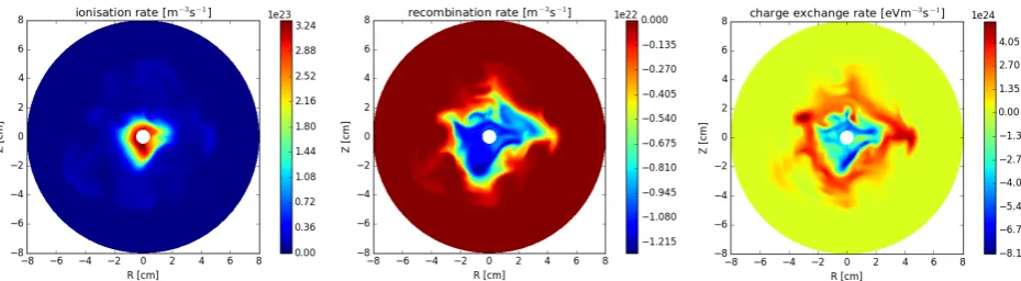
Figure 5. Contours of the ionisation (left) and recombination (middle) density rates per cubic metre, and charge exchange energy source (right) are shown 1m down the linear device for a single time slice. The recombination is negative because it acts as a sink for the plasma density. The charge exchange demonstrates that the plasma heats the neutrals at the centre of the device, while the neutrals heat the plasma towards the edge.

4.2 Localisation of interactions

The existence of turbulence strengthens the interaction between neutrals and plasma, and it also changes the location of these interactions. With Gaussian profiles, symmetric axially about the device, the interaction is also symmetrical. However, with turbulence, the location of the interactions can change significantly, as shown in figure 5. The mean free path of the neutrals for ionisation is large, on the order of the machine size, so the ionisation source does not show strong features from the turbulence. The maximum is at the areas of highest plasma density and temperature, and the features are blurred. For recombination, however, the mean free path is much smaller, on the order of a centimetre, so the sink is correlated with the intricate features of the plasma turbulence. This process occurs strongest in the areas of high density but low temperature. The energy transfer between neutrals and plasma due to charge exchange is shown in the right plot of figure 5. An interesting flow of energy can be seen - the plasma loses energy to the neutrals at the hottest regions (ie. near the centre of the plasma column), and gains energy from the neutrals at the plasma edge in the lowest temperature regions.

5 Conclusion

Acknowledgements

Some of the simulations were run using the ARCHER computing service through the Plasma HEC Consortium EPSRC grant number EP/L000237/1. This work has received funding from the RCUK Energy Programme, grant number EP/I501045. It has been carried out within the framework of the EUROfusion Consortium and has received funding from the Euratom research and training programme 2014-2018 under grant agreement No 633053. The views and opinions expressed herein do not necessarily reflect those of the European Commission.

References

[1] T. Hirai, H. Maier, M. Rubel, Ph. Mertens, R. Neu, E. Gauthier, J. Likonen, C. Lungu, G. Maddaluno, G.F. Matthews, R. Mitteau, O. Neubauer, G. Piazza, B. Riccardi, C. Ruset, and I. Uytdenhouwen. R&D on full tungsten divertor and beryllium wall for JET ITER-like wall project. Fusion Engineering and Design, 82(15-24):1839–1845, October 2007.

[2] V. Kotov, D. Reiter, R. A. Pitts, S. Jachmich, A. Huber, D. P. Coster, and JET-EFDA Contributers. Numerical modelling of high density JET divertor plasma with the SOLPS4 . 2 ( B2-EIRENE ) code. Plasma Physics and Controlled Fusion, 105012(50), 2008.

[3] P. Stangeby. The plasma boundary of magnetic fusion devices. Institute of Physics Pub., 1 edition, 2000.

[4] Y. Marandet, A. Mekkaoui, D. Reiter, P. Boerner, P. Genesio, J. Rosato, H. Capes, F. Catoire, M. Koubiti, L. Godbert-Mouret, and R. Stamm. Effects of turbulent fluctuations with prescribed statistics on passive neutral particle transport in plasmas. Plasma Physics and Controlled Fusion, 53:065001, 2011.

[5] F. Guzman, Y. Marandet, P. Tamain, H. Bufferand, G. Ciraolo, P.H. Ghendrih, R. Guirlet, J. Rosato, and M. Valentinuzzi. Ionization balance of impurities in turbulent scrape-off layer plasmas I: local ionization-recombination equilibrium. Plasma Physics and Controlled Fusion, 57:125014, 2015.

[6] A. N. Simakov and P. J. Catto. Drift-ordered fluid equations for modelling collisional edge plasma. Contributions to Plasma Physics, 44(1):83–94, 2004.

[7] B.D. Dudson, M.V. Umansky, X.Q. Xu, P.B. Snyder, and H.R. Wilson. BOUT++: A framework

for parallel plasma fluid simulations. Computer Physics Communications, 180(9):1467–1480,

September 2009.

[8] R. Fitzpatrick. The Physics of Plasmas. Lulu, 2008.

[9] S. Braginskii. Transport Processes in a Plasma. Reviews of Plasma Physics, 1:205–311, 1965.

[10] L. Spitzer and R. H¨arm. Transport phenomena in a completely ionized gas. Physical Review

Letters, 89:977–980, 1953.

[11] D. Reiter, M. Baelmans, and P. B¨orner. The eirene and b2-eirene codes. Fusion Science and Technology, 47(2):172–186, 2005.

[12] D. Coster, X. Bonnin, G. Corrigan, and S. Wiessen. Edge codecode benchmarking. In ITPA -DivSOL, 2007.

[13] F. Wising, D.A. Knoll, S.I. Krasheninnikov, T.D. Rognlien, and D.J. Sigmar. Detachment in ITER-Geometry Using the UEDGE Code and a Fluid Neutral Model. Contributions to Plasma Physics Plasma Physics, 36:309–313, 1996.

[14] M. V. Umansky, T. D. Rognlien, M. E. Fenstermacher, M. Borchardt, A. Mutzke, J. Riemann, R. Schneider, and L. W. Owen. Modeling of localized neutral particle sources in 3D edge plasmas. Journal of Nuclear Materials, 313-316:559–563, 2003.

[15] D. R. Bates, A. E. Kingston, and R. W. P. Whirter. Recombination between electrons and atomic ions. Proceedings of the Royal Society of London. Series A, mathematical and Physical Sciences., 267:297–312, 1962.

[16] R.K. Janev. Elementary processes in hydrogen-helium plasmas: cross sections and reaction rate coefficients. Springer series on atoms + plasmas. Springer-Verlag, 1987.

[17] T.D. Rognlien, P.N. Brown, and R.B. Campbell. 2D Fluid Transport Simulations of

Gaseous/Radiative Divertors. Contributions to Plasma Physicsto Plasma Physics, 34:362–367, 1994.

[18] G. De Temmerman, J. Daniels, K. Bystrov, M.A. van den Berg, and J.J. Zielinski.

Melt-layer motion and droplet ejection under divertor-relevant plasma conditions. Nuclear Fusion, 53(2):23008, 2013.

[19] J. Loizu, P. Ricci, F. D. Halpern, and S. Jolliet. Boundary conditions for plasma fluid models at the magnetic presheath entrance. Physics of Plasmas, 19(2012), 2012.