for surface deformation estimation.
White Rose Research Online URL for this paper:
http://eprints.whiterose.ac.uk/101242/
Version: Accepted Version
Article:
Li, J.T., Xu, H.P., Shan, L. et al. (2 more authors) (2016) An efficient compressive sensing
based PS-DInSAR method for surface deformation estimation. Measurement Science and
Technology, 27. 114001. ISSN 0957-0233
https://doi.org/10.1088/0957-0233/27/11/114001
[email protected] https://eprints.whiterose.ac.uk/ Reuse
Unless indicated otherwise, fulltext items are protected by copyright with all rights reserved. The copyright exception in section 29 of the Copyright, Designs and Patents Act 1988 allows the making of a single copy solely for the purpose of non-commercial research or private study within the limits of fair dealing. The publisher or other rights-holder may allow further reproduction and re-use of this version - refer to the White Rose Research Online record for this item. Where records identify the publisher as the copyright holder, users can verify any specific terms of use on the publisher’s website.
Takedown
If you consider content in White Rose Research Online to be in breach of UK law, please notify us by
An Efficient Compressive Sensing Based PS-DInSAR Method for
Surface Deformation Estimation
J T Li1,2, H P Xu*1, L Shan1 , W Liu3 and G Z Chen4 1
School of Electronic and Information Engineering, Beihang University, Beijing, China
2
Sino-French Engineering School, Beihang University, Beijing, China
3 Department of Electronic and Electrical Engineering, University of Sheffield, Sheffield, S1 3JD, UK
4 Shanghai Institute of Satellite Engineering, Shanghai, China
* Corresponding Author
E-mail: [email protected]; [email protected]; [email protected];
[email protected]; [email protected]
Abstract. Permanent scatterers differential interferometric synthetic aperture radar (PS-DInSAR) is a
technique for detecting surface micro-deformation, with an accuracy at the centimeter to millimeter level. However, its performance is limited by the number of SAR images available (normally more than 20 are needed). Compressive Sensing (CS) has been proven to be an effective signal recovery method with only a very limited number of measurements. Applying CS to PS-DInSAR, a novel CS-PS-DInSAR method is proposed to estimate the deformation with fewer SAR images. By analyzing the PS-DInSAR process in detail, first the sparsity representation of deformation velocity difference is obtained; then, the mathematical model of CS-PS-DInSAR is derived and the restricted isometry property (RIP) of the measurement matrix is discussed to validate the proposed CS-PS-DInSAR in theory. The implementation of CS-PS-DInSAR is achieved by employing basis pursuit algorithms to estimate the deformation velocity. With the proposed method, DInSAR deformation estimation can be achieved by a much smaller number of SAR images, as demonstrated by simulation results.
Keywords: Permanent scatterer; DInSAR; Compressive Sensing; Deformation
1.Introduction
Differential interferometric synthetic aperture radar (DInSAR) is a technique to estimate surface deformation, and has a remarkable achievement in geodynamics. Its accuracy has reached the centimeter to millimeter level.
By selecting highly coherent targets over long time intervals, the long time series DInSAR was developed to
eliminate the influence caused by time decorrelation and the atmospheric phase, and thus able to estimate the surface micro-deformation with very high precision.
Thanks to the large amount of data from satellite and the improved capability of satellite SAR sensors (Cosmo-SkyMed, RADARSAT, TerraSAR-X/Tandem-X) including resolution and revisit time, the long time series DInSAR technique has been a great success. Wasowski et al. discussed issues and future directions for landslides and unstable slope investigation using this technique [1], while Peduto et al. presented a general framework with related procedures for DInSAR in the domain of subsidence analysis for different scale areas [2]. There are three main methods for long time series DInSAR: Permanent Scaterrers (PS) DInSAR [3], Small Baseline Subset (SBAS) [4], and coherent target (CT) [5].
for space baseline is strict and the atmospheric effect is not considered before estimating the linear deformation velocity. The CT technique was proposed in [5] in 2003, which selects PS candidates by thresholding the value of correlation, and chooses more than one master images to generate the interferometric pairs. The method can reduce the number of SAR images to some extent. Nevertheless, a large number of SAR images are required to estimate the non-linear deformation velocity.
Ferretti et al. proposed the PS-InSAR technique in 1999 [3], and studied the landslide of the Ancona area (5km ×5km) in Italy by 34 ERS SAR images. Time span of these images was more than five years. The detected deformation was 3mm/year. Later, Ferretti et al. proposed an improved technique to study the Pomina area of California, USA [6], which was a 16km × 20km area in 2000. 41 ERS SAR images were used and the time span was more than six years. The improved method helped to solve the estimation problem of non-linear deformation velocity. The method estimates the deformation velocity by searching for the optimal combination in the solution space [7]. Kampes and Hanssen proposed the LAMBDA (least square ambiguity decorrelation adjustment) method in 2004 in order to overcome the disadvantages of the method [8]. The StaMPS (Stanford Method for Persistent Scatterer) method was proposed by Hooper et al in 2006 [9], which sets up a full suite of PS-DInSAR processing. The deformation phase can be obtained after 3-D unwrapping and removing the error phase.
A sufficient number of SAR images (>20) should be available to have a reliable estimation of the studied movement using the PS-DInSAR technique. However, spaceborne SAR images are usually obtained by repeating orbits, which will take a long time, and it will be very difficult to estimate the deformation in time. For instance, Deffontaines B et al. used 40 ERS SAR images to study the deformation of Montmartre in France from 1993 to 1999 [10]. Liu Z G et al. monitored the subsidence caused by repeated mining in Gujiao County in China with 27 Terra-SAR images from 2012 to 2013 [11].
So far, PS-DInSAR has been able to achieve a high accuracy of estimation. Nevertheless, the time span is too long because of large number of required SAR images. Even though the revisit time is from 11 to 4 days for X-band acquisition, the time span is just reduced from several years to several months. The improvement is limited and the long data acquisition time (i.e. number of SAR images) is still a problem for PS-DInSAR. For example, 14 images are needed in [1] and ~30 in [2].
In recent years, Compressive Sensing (CS) has been proposed for effective signal reconstruction from far fewer measurements by employing the sparsity property of the signal [12], and it has been applied to a wide range of areas.In this work, based on the CS theory, after analyzing the data sparsity of PS-DInSAR, a novel method, called CS-PS-DInSAR, is proposed.It can achieve a similar level of estimation accuracy with much smaller number of SAR images, which is demonstrated by two sets of simulation results.
The remainder of the paper is organized as follows. In Section 2, a review of PS-DInSAR and the CS theory is proposed, followed by a derivation of our proposed CS-PS-DInSAR in Section 3.Simulation results based on a simulated scene with a cone-shaped peak and a real scene of Xishan Mountain area in Beijing are provided in Section 4, including a detailed comparison with PS-DInSAR. Conclusions are drawn in Section 5.
2. PS-DInSAR method and CS theory 2.1 PS-DInSAR[6]
The SAR image is a 2D complex value ensemble which can be represented as: I = A . A is related to scattering intensity. carries the distance information between terrain target and the SAR sensor, i.e.
= − , where is sensor-target distance, and is system wavelength. With two or more SAR images of the same area, the interferogram can be generated by conjugate multiplication, i.e. In = I ∙ I∗ =
( ). The Interferometric phase can be represented: = − = − ( − ).
Furthermore, − = + !" + #$%+ & !"', where is the topographic feature with target elevation, !" is the displacement occurred between two SAR images’ acquisition time, #$% is the distance influenced by atmospheric phase screen (APS) and & !"' is the decorrelation source.
is contribution from the interferometric phase. It can be eliminated by digital elevation models (DEMs) or differential processing with other interferogram of the same area, and then the terrain deformation
PS-DInSAR [6] chooses the points which are coherent over long time intervals as PS points from a temporal series SAR images. The phase information can be obtained from these sparsely distributed PS candidates, and then reliable deformation velocity measurements can be estimated.
Suppose there are in total S SAR images to be processed. Firstly, one of the S SAR images is considered as the reference “master”. And then S-1 interferometric SAR images are generated by the interferometry of the other S-1 slave images with the master image respectively. After isolating the topographic contribution, S-1 differential interferograms are obtained.
The differential interferometric phase can be represented as [6]:
φ !)(*+, -) = ./,0∙ 1(*+) + .2,0∙ 3(*+) + /45(*+, -) + 6(*+, -) + 7(*+, -) (2.1)
where ./,0= ∙ 80, .2,0 = < "!& =9:; , *+ is the PS candidate, - is the sequence number of differential interferograms with - ∈ [1, A − 1], 80 is the temporal baseline, CD0 is the normal baseline value with
respect to the master orbit, 1 is the mean deformation velocity of the PS candidate, 3 is the digital elevation model (DEM) error, /EF represents phase contribution from nonlinear motion, 6 means APS, and 7 is the decorrelation noise.
The phase difference of the adjacent PS candidates (*+, *) is studied:
Δ !)H*+, * , -I = ./,0∙ Δ1+ + .2,0∙ ∆3+ + ∆ K'",0 (2.2)
with ∆ K'",0= /EF(*+, -) − /EFH* , -I + 6(*+, -) − 6H* , -I + 7(*+, -) − 7H* , -I (2.3) where Δ1 is deformation velocity difference of adjacent PS candidates, ∆3 is DEM error difference of adjacent PS candidates, and ∆ K'",0 is the phase residue including atmospheric effects, nonlinear deformation and noise phase.
The surface nonlinear deformation and the influence of APS are both highly spatially correlated, which results in small differences of neighboring PS candidates ∆ /EF= /EF(*+, -) − /EFH* , -I and ∆6 =
6(*+, -) − 6H* , -I. Furthermore, the noise is almost not affected by time and spatial decorrelation due to the
strong coherence of PS candidates. So ∆7 = 7(*+, -) − 7(* , -) is also small. Consequently, the phase residue is considered as a small quantity [6].
As the value of ∆ K'" tends to zero, the problem of estimating (∆3, Δ1) is then transformed into finding the 2-D frequency of the complex sinusoid representation of Δ !)H*+, * , -I. Basically, the optimal solution is deduced by maximizing the phase coherence coefficient γ based on the S-1 differential interferograms [6]:
M∆3N, Δ1N P = arg maxγ(∆3,Δ1) (2.4)
γ(∆3, Δ1) = V% ∑%0[ exp (j ∙ ∆ K'",0)V = V% ∑%0[ exp {j ∙ ]Δ !)H*+, * , -I − ./,0∙ Δ1 − .2,0∙ ∆3^}V (2.5)
where γ(∆3, Δ1) is the phase coherence of neighboring PS candidates, and j = √−1.
With the velocity difference, choosing a PS candidate as reference and giving its deformation velocity, the deformation velocities of every PS candidate can be estimated by integration.
2.2. Compressive Sensing Theory[12]
Consider a real-valued signal a ∈ ℝc and the basis d ∈ ℝc×c, with d providing a K-sparse representation of a = de, where Θ is an N×1 column vector with K nonzero elements. When K ≪ N, the signal a is compressible and is considered as a K-sparse signal.
The CS theory considers [12]:
g = ha = hde = ie (2.6) where g is a M×1 column vector; h is measurement M×N matrix with M<N. Signal a can be reconstructed by the optimal estimation of g based on l0-norm minimization.
In order to recover the signal exactly, the conditions of incoherence [13] and restricted isometry property (RIP) [14] should be satisfied. The orthogonal basis d and the measurement matrix h must be incoherent, which means the rows of matrix d cannot be linearly represented by the columns of matrix h and vice versa.
For a K-sparse signal a, RIP is defined by the following formula [14]:
where kl is a small number as the isometry constant of measurement matrix h. This property requires that all K columns submatrix of h are nearly orthogonal.
Although the RIP in (2.7) is hard to verify in practice, [15] proposed an equivalent method. The incoherence and RIP requirements can be represented as that any 2K columns of A should be uncorrelated [15] where p = hd ∈ ℝq×c. Since A shows the relationship between y and e, A is referred to as transformed dictionary or sensing matrix.
In practice, the measured signal is always affected by small perturbations, leading to inaccuracy of reconstruction. Therefore, a model with added noise was studied in [12] as follows:
g = ha + r (2.8) where r ∈ ℝq× is the noise vector.
As the l0-norm of a vector is the vector’s sparsity, the recovery of signal is carried out by the following l0-norm minimization [16]:
as = arg min‖a‖u-. w. g = ha (2.9) However, solving the above problem needs a combinatorial enumeration of the HclI possible sparse subspace, which is known to be NP-hard. Basis pursuit (BP) [17] and matching pursuit (MP) [18] are two main ideas to solve this problem.
BP method transforms the problem into l1-norm minimization based on the incoherence of bases. It can be solved easily by linear programming techniques. The signal a can be reconstructed by the following formula [17]:
as = arg min‖x‖ -. w. g = ha (2.10) The calculation of l1- norm minimization is complicated but highly accurate.
MP [18], called as greedy iteration, uses the relation between signal and an atom dictionary to obtain the non-zero atom. The algorithm selects local optimal solutions by iteration and then recovers the signal. In 2007, Joel Tropp and Anna Gilbert proposed orthogonal matching pursuit (OMP) [19] based on MP and the CS theory. OMP can reconstruct the signal with a high accuracy. Compared with the BP algorithm, the realization of MP algorithm is easier and faster, but less accurate.
3. Our method
3.1. CS-PS-DInSAR
Rewrite Δ !)H*+, * , -I in (2.2) as:
Δ !)H*+, * , -I = [./,0 .2,0] yΔ1∆3+
+ z + ∆ K'",0 (3.1) The similarity of the above formula and the formula (2.8) inspires us to employ the CS theory as an estimation method for (Δ1, ∆3).
The following sub-subsections provide an analysis of the sparsity of deformation velocity and the mathematical model combined with CS theory to estimate (Δ1, ∆3) with fewer SAR images.
3.1.1. Sparsity of deformation velocity
The sparsity of the signal is the key to verify the applicability of the CS theory in CS-PS-DInSAR. The
parameters to be estimated are velocity differences between neighboring PS candidates.
The PS-DInSAR technique selects PS candidates which are highly coherent. Furthermore, the distribution of the PS candidates is very tight. Consequently, the values of deformation velocities of neighboring PS candidates are close. The velocity difference Δ1 can be considered very small. Actually most of the Δ1 are
zero, which means that the values of Δ1 have a sparse distribution. Suppose that K values are non-zero while the number of Δ1 is N (N>K). Here, K is the sparsity of data.
These conditions suggest that (Δ1, ∆3) could be reconstructed using the CS theory, given that Δ1 is K-sparse.
3.1.2. Mathematical model
{ | | | |
}ΔΔ !), ,
!), ,
⋮ Δ !), ,c
⋮ Δ !),q,c•
€ € € € • = { | | | | | |
} ./, 0
⋱
0 ./,
.2, 0
⋱
0 .2,
⋮
./,q 0
⋱
0 ./,q
⋮
.2,q 0
⋱
0 .2,q•€
€ € € € € • { | | | | }Δ1⋮
Δ1c
∆3 ⋮ ∆3c•
€ € € € • + { | | | |
}ΔΔ K'", ,
K'", ,
⋮ Δ K'", ,c
⋮ Δ K'",q,c•
€ € € € • (3.2)
As .2,„= < "!& =9:… , ∆3„can be replaced by ∆†„ with ∆†„= < "!&=∆‡… . Therefore, the above formula is transformed into: { | | | | }ΔΔ !), ,
!), ,
⋮ Δ !), ,c
⋮ Δ !),q,c•
€ € € € • = { | | | | | |
} ./, 0
⋱
0 ./,
CD 0
⋱
0 CD
⋮
./,q 0
⋱
0 ./,q
⋮
CDq 0
⋱
0 CDq•€
€ € € € € • { | | | | }Δ1⋮
Δ1c
∆† ⋮ ∆†c•
€ € € € • + { | | | |
}ΔΔ K'", ,
K'", ,
⋮ Δ K'", ,c
⋮ Δ K'",q,c•
€ € € € • (3.3)
The representation can be simplified as
∆ˆ = ‰Š + ∆‹K'" (3.4)
Where Œ is the number of differential interferograms, Nis the number of Δ1 after construction of Delaunay triangulation [20, 21], ∆ˆ is an (Œ × •) ×1 column vector, ‰ is an (Œ × •) × (• × 2) matrix
pre-determined by system parameters, Š = y•••‘z is an (• × 2) × 1 column vector which is the matrix to be
estimated, and ∆‹K'" is an (Œ × •) ×1 column vector holding phase residues.
Here, the sparse base is Dirac base, which is an (• × 2) × (• × 2) identity matrix I. The transformed matrix can be obtained by ‰ × ’ = ‰. The property of C is analyzed in the following:
‰“‰ = { | | | | | |
}./, 0
⋱
0 ./,
… ./,q ⋱ 0
0 ./,q
CD 0
⋱
0 CD
…
⋮
CDq 0
⋱
0 CDq•
€ € € € € € • { | | | | | |
} ./, 0
⋱
0 ./,
CD 0
⋱
0 CD
⋮
./,q 0
⋱
0 ./,q
⋮
CDq 0
⋱
0 CDq•
€ € € € € € • (3.5)
To verify the RIP and incoherence of ‰, the correlation of 2K columns in ‰ is analyzed, where K is the sparsity of Š but unknown in practice. Thus, the determinant of ‰“‰ is calculated. If |‰“‰| > 0, any two columns of ‰ are uncorrelated, which means for any K, the requirement is met.
det (‰“‰) =
™ ™ ™ | | | | | | | | | |
} š ./,›
q
„[ 0
⋱
0 š ./,›
q
„[
š ./,›CD„
q
„[ 0
⋱
0 š ./,›CD„
q
„[
š ./,›CD„
q
„[ 0
⋱
0 š ./,›CD„
q
„[
š CD„
q
„[ 0
⋱
0 š CD„
q „[ € € € € € € € € € € • ™ ™ ™
year depending on the revisit time of satellite. Thus, the range of ./,„ is 10u~10 with ./,„= ∙ 8„.
And the range of CD„ is 10 ~10 m, consequently, ∑q„[ ./,› ∙ ∑„[q CD„ > 1 and ∑q„[ ./,›CD„ >
1. These two conditions lead to that ]∑q„[ ./,› ∙ ∑q„[ CD„ ^c≥ H∑q„[ ./,›CD„I c, i.e. det (‰“‰) ≥ 0. Since 8„ and CD„ are different for different SAR image, .2,„ ¡ .2,„ , and CD„ ¡ CD„ , then the equality does not hold, i.e. det (‰“‰) ¡ 0. Consequently, |‰“‰| > 0, i.e., RIP and incoherence of ‰ are satisfied and the deformation velocity can be recovered under the CS framework.
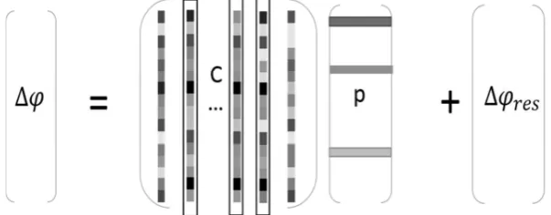
The estimation of Δ1 based on sparsity is shown in Figure 1, where the colored elements in p are large coefficients. As the distribution of Δ1 is sparse, vector p can be reconstructed accurately with these large coefficients according to CS theory. The number of measurements, i.e. the matrix row number: Œ × • of
∆ˆ, can be reduced thanks to the sparsity of p, which means that the number of differential interferograms M can be reduced because N is determined once the selection criteria of PS candidates are determined.
Meanwhile, the accuracy of the result is maintained by the sparse estimation. Therefore, y•••‘z can be
[image:7.595.155.457.325.443.2]estimated by fewer differential interferograms. Then, the purpose of reducing the originally required number of SAR images is achieved.
Figure 1. Graphic illustration: the mathematical model of CS.
3.1.3. Reconstruction algorithm
Depending on the signal reconstruction principal of MP [19] and OMP [20], the residue of each iteration includes the noise energy, which may lead to non-optimal iteration result. Then, the final estimation of Δ1 may have a deviation from the true value. As a result, MP and OMP are not the best candidates for this case.
On the other hand, since the BP algorithm does not have the noise energy accumulation problem, it is
adopted here. According to the model in (2.10), y•••‘z is the sparse signal which can be estimated by the
following formula with fewer SAR images:
Š¢ = y•••‘NN z = arg min £•••‘£ = arg min‖‰ ∙ ∆ˆ‖
= arg min ™ ™ ™
{ | | | | | |
} ./, ⋱ 0
0 ./,
CD 0
⋱
0 CD
⋮
./,q 0
⋱
0 ./,q
⋮
CDq 0
⋱
0 CDq•€
€ € € € € •
∙
{ | | | | }ΔΔ !), ,
!), ,
⋮ Δ !), ,c
⋮ Δ !),q,c•€
€ € € •
™ ™ ™
(3.7)
The sparsity of Δ1 cannot be determined in advance and the influence of residue phase ∆ ¤¥0 is considered as noise. By the BP algorithm [23], the problem is transformed into the following optimization problem:
min ™ ™ { | | | | | |
} ./, 0
⋱
0 ./,
CD 0
⋱
0 CD
⋮
./,q 0
⋱
0 ./,q
⋮
CDq 0
⋱
0 CDq•€
€ € € € € • { | | | | }Δ1⋮
Δ1c
∆† ⋮ ∆†c•
€ € € € • − { | | | |
}ΔΔ !), ,
!), ,
⋮ Δ !), ,c
⋮ Δ !),q,c•
€ € € € • ™ ™ + ¦ ™ ™ { | | | | }Δ1⋮
Δ1c
∆† ⋮ ∆†c•
€ € € € • ™ ™ (3.9)
where α > 0 is the regularization parameter for Tikhonov regularization [24].
With the result of (Δ1,∆†), ∆3 = < "!& =∆†, and 1 can be estimated using the same process of PS-DInSAR.
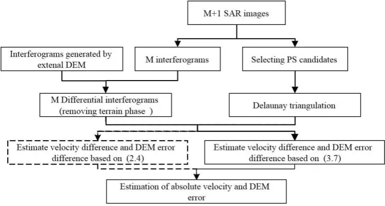
3.2.Processing procedure
The whole processing procedure is shown in Figure 2. M+1 SAR images are used, with one of them chosen as the master image and the others as slave images. After the interferometry operation, we have M interferograms I1. At the same time, another M interferograms I0 that represent the terrain phase are generated by external
DEM. Then, the differential interferograms without terrain phase can be obtained by differential processing between I1 and I0. On the other hand, PS candidates are selected by the amplitude thresholding value method
[3] based on the M+1 SAR images. Based on the differential phase model of neighboring PS candidates, a network is built to determine the relationship of neighboring PS points. The network is constructed with fewer sides meaning fewer PS point pairs and less computation by Delaunay triangulation, details of which can be found in [20, 21].
Next, the velocity difference and DEM error are jointly estimated based on differential interferograms with (3.7). Finally, the absolute velocities and DEM errors of the PS points are obtained by integration.
[image:8.595.101.496.449.660.2]The step of PS-DInSAR in [6] is also shown in Figure 2 marked with dashed frame, where phase coherence maximization in (2.4) is performed instead of employing (3.7).
Figure 2. Processing procedure of the proposed CS-PS-DInSAR.
4. Simulation
4.1. Simple scene
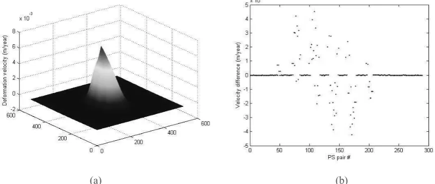
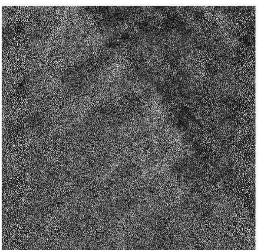
scene is set as Figure 3(a), where the height of the peak grows at a rate of 0.01m per year. 110 scatterers with larger backscatter coefficient are emplaced as permanent scatterers and are uniformly distributed at the whole scene. One of the generated SAR images is shown in Figure 3(b).
[image:9.595.105.512.169.346.2]
(a) (b)
Figure 3. Simple scene settings: (a) the theoretical motion of scene; (b) one of Generated SAR image of simple scene.
17 SAR images are generated by repeating orbit model. The parameters of baselines are showed in Table 2. The 9th image is chosen as the master image and the rest are slave images. After the processing of interferometry and differential interferometry, a 2D Delaunay triangulation of PS has been created. The surface deformation velocities are calculated using our proposed method with continuous sampling near the master image (e.g., choosing 7th, 8th, 9th, 10th images). The estimated deformation velocity is shown in Figure 4(a).Compared with the theoretical result in Figure 3, we can see that both values are 0.0076m/year in the LOS (line of sight) direction. The velocity difference distribution of neighboring PS candidates is given in Figure 4(b). Clearly, as expected, most values of velocity difference are zero.
[image:9.595.80.518.490.675.2](a) (b)
Figure 4. (a) Estimated deformation velocity with CS-PS-DInSAR; (b) The velocity difference distribution of neighboring PS candidates.
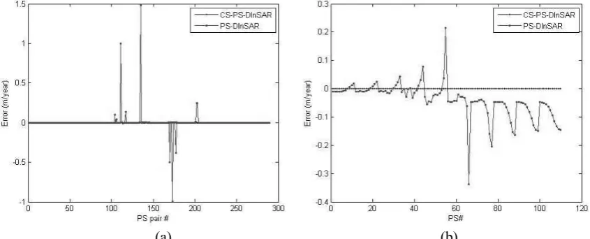
To have a fair comparison between the proposed method and the PS-DInSAR method, the same number of SAR images, which is 4, are used. The deformation velocity difference errors of these two methods, by calculating the difference between the real velocity difference value and the estimated results, are shown in
deformation velocity estimation errors of both methods are shown in Figure 5(b).A quantitative comparison is presented in Table 3. The average error by the proposed method is 1.1907 × 10 ªm/year, while that of the PS-DInSAR is 0.0727m/year.
[image:10.595.94.517.173.344.2](a) (b)
Figure 5. Comparison of deformation velocity difference error and deformation velocity error for a simple scene.
Secondly, in order to reduce estimation error, the number of SAR images in the PS-DInSAR method is increased. Since it is unlikely to reach exactly the same level of accuracy by both PS-DInSAR and our
proposed method, the value of 10 ~10 ªm/year is treated as a common standard for both methods. Table 4 shows the result for the number of SAR images and computing time. We can see that for PS-DInSAR, it requires at least 11 SAR images for the average error to reach the 10 m/year level; for our method, it only
needs 4 SAR images and the average error is 1.1907 × 10 ªm/year. On the other hand, the computation time of our proposed method and PS-DInSAR is 0.1977s and 12.8613s, respectively, which means that the proposed method is not only better in estimation accuracy, but also much faster with a very low computational complexity.
4.2. Complex scene
Figure 6. Generated SAR images for a complex scene.
Table 2. Simulation parameters for the simple and complex scenes.
Simple scene Complex scene
Time series
Horizontal baseline(m)
Normal baseline(m)
Temporal baseline(year)
Time series
Horizontal baseline(m)
Normal baseline(m)
Temporal baseline(year)
1 94 215 -4 1 0 0 0
2 -150 -353 -3.5 2 92.5722 253.9823 0.5
3 -100 -290 -3 3 81.6462 178.8132 1
4 9 119 -2.5 4 -148.555 -307.007 1.5
5 75 200 -2 5 -99.2294 -170.083 2
6 60 150 -1.5 6 152.4396 -121.244 2.5
7 -90 -185 -1 7 86.7405 -150.161 3
8 -80 -164 -0.5 8 143.8785 -245.153 3.5
9 0 0 0 9 -143.805 204.8258 4
10 86 209 0.5 10 137.5982 -192.94 4.5
11 18 105 1 11 87.1477 301.4231 5
12 -150 -353 1.5 12 -85.9948 122.4846 5.5
13 -70 -88 2 13 -75.8304 -109.519 6
14 70 250 2.5 14 -72.6985 121.2196 6.5
15 80 200 3 15 -132.734 -127.426 7
16 100 100 3.5 16 -63.3329 -118.306 7.5
17 50 100 4 17 -76.5142 -277.877 8
[image:12.595.79.524.125.330.2]
(a) (b)
Figure 7. Interferogram and differential interferogram.
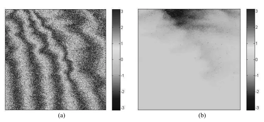
After secleting PS candidates, the built Delaunay triangulation is shown in Figure 8(a). By the model in (3.3), the PS point pairs’ velocity differences are estimated. Their distribution in Figure 8(b) shows that most values are almost zero, indicating a sparse result has been obtained.
(a) (b)
Figure 8. (a) Delaunay triangulation base on PS candidates; (b) Distribution of velocity difference of PS pairs.
Several control points have been set in the scene, and their deformation velocities in the LOS direction will be given by the SAR image generation. The control points’ deformation velocities are considered as the theoretical values.
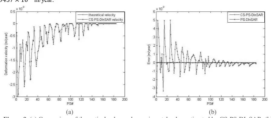
By choosing the first four SAR images, the deformation velocities of PS points estimated by the CS-PS-DInSAR method are compared with their theoretical values. The comparison result is shown in Figure
9(a), where the largest deformation velocity basically agrees well with the theoretical value which is 0.003m/year.
Next, the estimation result is compared with that of the traditional PS-DInSAR. The first comparison is
[image:12.595.85.533.396.594.2]0.0011m/year. On the other hand, the proposed method is more accurate, with an average error of only
8.9457 × 10 ±m/year.
[image:13.595.73.522.144.340.2](a) (b)
Figure 9. (a) Comparison of theoretical value and experimental value estimated by CS-PS-DInSAR; (b) Comparison of deformation velocity error between PS-DInSAR and CS-PS-DInSAR.
The second comparison is based on the same level of estimation accuracy for the deformation velocity, which is roughly 10 ±m/year. Table 4 shows the result of required image number and computing time. PS-DInSAR and our method need at least 12 SAR and 4 SAR images, respectively, when the average error of PS-DInSAR and our method is 7.5192 × 10 ±m/year and 8.9457 × 10 ±Ÿ/² 6³, respectively. The computing time of our method and PS-DInSAR is 0.4505s and 20.703s, respectively.
Table 3. Accuracy comparison with the same number of SAR images Type of
scene
Accuracy of PS-DInSAR(m/year)
Accuracy of CS-PS-DInSAR(m/year) simple
scene
0.0727 1.1907 × 10 ª
complex scene
[image:13.595.59.536.549.612.2]0.0011 8.9457 × 10 ±
Table 4. Required number of SAR images and computing time with the same level of accuracy
Type of method
SAR image number to achieve the same
accuracy Computing time(s)
Simple scene Complex scene Simple scene Complex scene
PS-DInSAR 11 12 12.8631 13.998
CS-PS-DInSAR 4 4 0.1977 0.4505
5. Conclusions
A compressive sensing based PS-DInSAR method has been proposed for effective deformation estimation in order to reduce data redundancy and improve the efficiency of data processing. As demonstrated by detailed simulation results, a high surface deformation velocity estimation accuracy can be achieved by the proposed method with a much smaller number of SAR images in comparison with the traditional PS-DInSAR method. Moreover, the running time of the proposed method is also much shorter.
6. Acknowledgement
This work is funded by the Natural Science Foundation of China (no. 61471020), China Aerospace Science and Technology Corporation (CASC) and the Program for New Century Excellent Talents in University.
Reference:
[1] Wasowski J, and Bovenga F 2014 Investigating landslides and unstable slopes with satellite multi temporal interferometry: current issues and future perspectives J. Engineering Geology. 174(8) 103-138
[2] Peduto D, Cascini L, Arena L, Ferlisi S, Fornaro G, and Reale, D 2015 A general framework and related procedures for multiscale analyses of dinsar data in subsiding urban areas J. Isprs Journal of Photogrammetry & Remote Sensing.105 186-210
[3] Ferretti A, Prati C, and Rocca F 2001 Permanent scatterers in SAR interferometry J. Geoscience and Remote Sensing, IEEE Transactions on.39(1) 8-20
[4] Berardino P, Fornaro G, Lanari R, and Sansosti E 2002 A new algorithm for surface deformation monitoring based on small baseline differential SAR interferograms J. Geoscience and Remote Sensing, IEEE Transactions on.40(11) 2375-2383
[5] Mora O, Mallorqui J J, and Broquetas A 2003 Linear and nonlinear terrain deformation maps from a reduced set of interferometric SAR images J. Geoscience and Remote Sensing, IEEE Transactions on. 41(10) 2243-2253
[6] Ferretti A, Prati C, and Rocca F 2000 Nonlinear subsidence rate estimation using permanent scatterers in differential SAR interferometry J. Geoscience and Remote Sensing, IEEE transactions on. 38(5) 2202-2212
[7] Colesanti C, Ferretti A, Novali F, Prati C, and Rocca F 2003 SAR monitoring of progressive and seasonal ground deformation using the permanent scatterers technique J. Geoscience and Remote Sensing, IEEE Transactions on.41(7) 1685-1701
[8] Kampes B M, and Hanssen R F 2004 Ambiguity resolution for permanent scatterer interferometry J. Geoscience and Remote Sensing, IEEE Transactions on.42(11) 2446-2453
[9] Hooper A, Segall P, and Zebker H 2007 Persistent scatterer interferometric synthetic aperture radar for crustal deformation analysis, with application to Volcán Alcedo, Galápagos J. Journal of Geophysical Research: Solid Earth (1978–2012).112 B7
[10] Deffontaines B, Fruneau B, and Leparmentier A M 2004 Urban Instability Revealed by DINSAR and PS Interferometry: The Montmartre Case Example (Paris, France) C. Proc. 2004 Envisat and ERS Symp(Salzburg,Austria). ESA SP-572
[11] Liu Z G, Bian Z F, Lei S G, Liu D L, and Sowter A 2014 Evaluation of PS-DInSAR technology for subsidence monitoring caused by repeated mining in mountainous area J. Transactions of Nonferrous Metals Society of China. 24(10) 3309-3315
[12] Candè E J, and Wakin M B 2008 An introduction to compressive sampling J. Signal Processing Magazine, IEEE.25(2) 21-30
[13] Candes E, and Romberg J 2007 Sparsity and incoherence in compressive sampling J. Inverse problems.23(3) 969
[14] Candes E J, and Tao T 2005 Decoding by linear programming J. Information Theory, IEEE Transactions on.51(12) 4203-4215
[15] Candès E J 2006 Compressive sampling J. Marta Sanz Solé.17(2) 1433-1452
[16] Candes E J, Romberg J, and Tao T 2006 Robust uncertainty principles: exact signal reconstruction from highly incomplete frequency information J. IEEE Transactions on Information Theory. 52(2) 489-509
[17] Donoho D L 2006 For most large underdetermined systems of linear equations the minimal ℓ1 norm solution is also the sparsest solution J. Communications on pure and applied mathematics. 59(6) 797-829
[19] Tropp J, and Gilbert A C 2007 Signal recovery from random measurements via orthogonal matching pursuit J. Information Theory, IEEE Transactions on.53(12) 4655-4666
[20] Delaunay B 1934 Sur la sphere vide J. Izv. Akad. Nauk SSSR, Otdelenie Matematicheskii i Estestvennyka Nauk.7(793-800) 1-2
[21] Yue H, Guo H, Chen Q, Hanssen R, Leijen F, Marinkovic P, and Ketelaar G 2005 Land subsidence monitoring in city area by time series interferometric SAR data. C. INTERNATIONAL GEOSCIENCE AND REMOTE SENSING SYMPOSIUM.7 4590
[22] Cauchy A 1821 Oeuvres 2 MIII p.373
[23] Kim S, Koh K, Lustig M, Boyd S, and Gorinevsky D 2007 A method for large-scale l1-regularized least squares problems with applications in signal processing and statistics J. IEEE J. Select. Topics Signal Process.1(4) 606-617