Modelling the effects of forest regeneration on streamflow using forest growth models

(1)

Modelling the effects of forest

regeneration on streamflow using

forest growth models

PhD dissertation

Dominik Jaskierniak, BSc GradDipSIS (Honours)

September, 2011

(University of Tasmania)

(2)

Declaration

This thesis contains no material which has been accepted for the award of any other degree or diploma in any tertiary institution, and to the best of my knowledge and belief, contains no material previously published or written by another person, except where due reference is made in the text of the thesis.

Signed

Yours Dominik Jaskierniak

Authority of Access

This thesis may be made available for loan and limited copying and communication in accordance with the Copyright Act 1968.

Signed

Yours Dominik Jaskierniak

Publications

The publisher of the paper comprising chapter 5 hold the copyright for that content, and access to the material may be sought from the respective journal. The published paper is titled:

(3)

Abstract

Forest regeneration is a dynamic process that affects forest hydrology through changes in structure and density of natural forests. In Victoria and Tasmania, forest hydrology models that manage the potential impacts of land cover disturbance on the water resource are not data-driven with information on vegetation dynamics that affect forest water use. Current models underutilise forest inventory databases for managing the forested water resources, even though available evidence suggests an inverse relationship between forest growth rates and long-term changes in

streamflow. This dissertation is the first published study that uses forest inventory data to produce spatiotemporal forest growth models to explain vegetation-induced streamflow trends. The study was undertaken in nine small catchments (7.4 to 52.8 ha) located in Melbourne’s Maroondah water catchment.

The hydrology model runs on an annual time step and partitions streamflow data into climate-induced noise using a climate filter, and vegetation-induced trend using an ellipse and gamma (“Kuczera curve”) function. A simulation exercise demonstrates how well the model structure isolates the vegetation-induced trend from climatic variability in streamflow using a range of synthesised scenario cases. The model framework allows for comparison of streamflow trends against a detailed forest growth model by using the same gamma function to quantify forest growth and vegetation-induced streamflow trends.

(4)

To temporally extrapolate stand volumes and basal area, LiDAR indices and permanent plot data were used in mixed effects models to capture the spatial heterogeneity in, and temporally polymorphic nature of forest growth. The

spatiotemporal models of forest growth were then lumped to the catchment-scale to represent changes in growth rates over the stream gauging period. The relationship between catchment-scale gamma parameters of forest growth and forest water use were explored, and results demonstrate that forest growth provides useful

(5)

Acknowledgements

I would like to thank many people for assistance and guidance during this research. First of all, I thank my supervisors Arko Lucieer and Richard Doyle for their

encouragement, patience, and overwhelming support throughout the project. Their diligence in overseeing the thesis is appreciated. My special thanks is also extended to my research advisors Patrick Lane and George Kuczera for their contribution in proof reading, editing, and providing specialist advice. Their forest hydrology expertise was invaluable at directing the project. I would also like to acknowledge with gratitude the office space and resources provided by Melbourne University and Newcastle University. Both opportunities provided ideal conditions for my science to progress with the support of colleagues from all over Australia. In the Forest and Water Group (Melbourne University) I am indebted to Richard Benyon, Patrick Mitchell, Paul Feikema, Chris Sherwin, Gary Sheridan, Phil Noske, and Huge Smith for their insight into forest hydrological systems. At the School of Civil Engineering (Newcastle University), I am grateful for the contribution Mark Thyre, Dmitri

Kavetski, and Tom Micevski made in overseeing the statistical computing challenges I faced.

I am also thankful for the forest inventory modelling insight Andrew Robinson and Owen Jones at the Mathematics Department (Melbourne University) provided. My gratitude is also extended to Rob Musk from Forestry Tasmania and Fiona Hamilton from Department of Sustainability of Environment for their support during the forest growth modelling exercises. For overseeing challenging statistical programming exercises I would also like to thank Simon Wotherspoon from the Mathematics Department (University of Tasmania).

A big thanks needs to go to Ian Watson for unearthing original field sheets of

(6)

Schmidt, Stan Jaskierniak, Sam Hoffman, Amy Rayner, and Michael Jaskierniak. For resolving computer issues I am indebted to Darren Turner.

(7)

List of Figures

1.1: The Kuczera Curve (with 90% confidence limits) predicting water yield decline from forest age in Mountain ash forests. Minimum yield is predicted to occur when the forest is 27 years old. P2.

2.1: The Gamma curve used by Kuczera (1985) to represent vegetation-induced reduction in streamflow. P9.

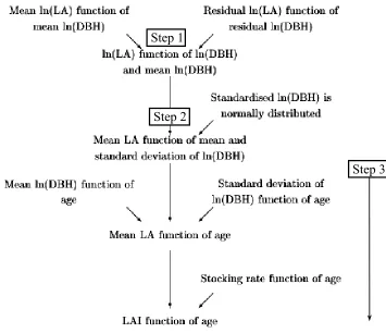
2.2: Flow chart summarising the steps taken to establish the relationship between LAI and age (from Watson, 1999). P11.

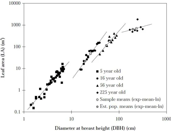
2.3: Sample LA versus DBH for four stands plotted on the log axis, which also provides; regression lines, sample means (white circles) and population means (grey circles) estimated from simple regression equations outlined below (from Watson, 1999). P12.

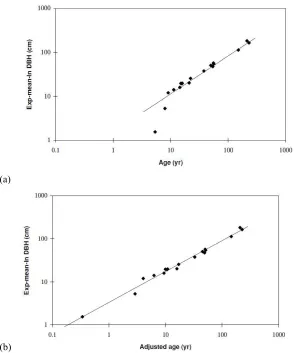
2.4: Logarithmic plot with the line of best fit for (a) In DBH versus ages, and (b) exp-mean-In DBH versus adjusted ages (from Watson, 1999). P13.

2.5: Histograms (using lines instead of bars) of ln(DBH) values within each stand; standardised and scaled to have zero mean, unit standard deviation, and unit area. A standard normal probability distribution function is provided for reference (from Watson, 1999). P14.

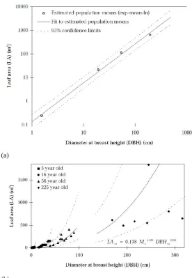
2.6 (a) Estimated variation in (estimated) population mean between stands ln(LA) and ln(DBH) and;

(b) LA versus DBH for the four stands with 95% confidence limits (dashed lines) (from Watson, 1999) P15.

2.7: Line of best fit for variance of In(DBH) versus age for each stand (from Watson, 1999). P16.

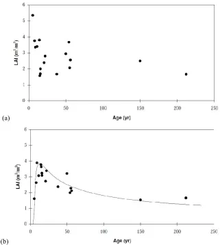
2.8: Predicted LAI versus age for healthy, fully stocked single-aged stands (a) uncorrected, and (b) corrected for variability in stocking rate and the final model is superimposed (from Watson, 1999). P17.

2.9: LAI:Age curve for E.regnans and mixed species (from Feikema et al., 2006). P18.

2.10: 50 m radius-averaged NDVI derived from shade corrected imagery plotted against ground measured LAI using a Li-Cor PCA (from Feikema et al., 2006). P20.

2.11: The relation between shade-corrected NDVI and forest age for E.regnans (from Feikema et al., 2006). P20.

2.12: Total LAI of E.regnans forest. The circles are ground measurements of LAI made using a Li-Cor PCA. The short thin lines are LAI values estimated using (shade-corrected) TNDVI derived from Landsat TM imagery. The long curved line is the predictive model (from Feikema et al., 2006). P21.

2.13: Stand sapwood area per unit leaf area, with power function fitted by linear regression (from Feikema et al., 2006). P22

2.14: Simulation of the Kuczera curve using Macaque supplied with synthetic, noiseless climate data (from Watson, 1999). P23.

(12)

2.16: An example of an ESU with an (a) acceptable annual water yield, (b) unacceptable annual water yield due to unexplained oscillations, and (c) unacceptable annual water yield due to prolonged zero water yield (from Feikema et al., 2006). P30.

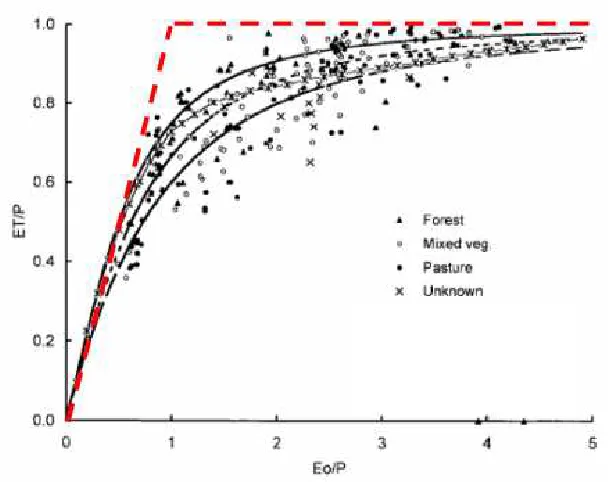
2.17: Maximum possible ET from a catchment using the ratio of mean annual ET to P as a function of the index of dryness (Eo/P). P32.

2.18: Dependence of the ratio of evaporation (E) to precipitation (r) upon the radiative index of dryness (R/Lr) (from Budyko, 1974). P33.

2.19: Ratio of mean annual evapotranspiration to rainfall as a function of the index of dryness (Eo/P) (from Zhang et al., 1999). P35.

2.20: Zhang curves predicting the relationship between annual ET and P for both forest and pasture (from Brown et al., 2006). P35.

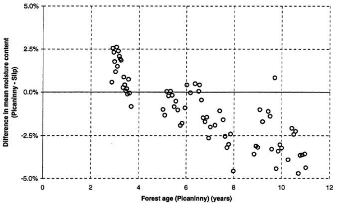
2.21: Effects of regeneration on soil moisture over time: represented as difference between a treated (Picaninny) and control (Slip) catchment (from Watson et al., 1999b). P37.

2.22: Response of Budyko curve to regenerating forest where; [1] represents an fast growing regenerating forest whereas [2] represents an old growth forest (from Donohue et al., 2006). P38.

2.23: Examples of how vegetation specific curves may be generated within the natural limit of the vegetation specific ecosystem with: A representing a tropical forest type, B represents a temperate vegetation type limited by the vegetations interaction with plant available water, and C representing an arid vegetation type. P39.

2.24: Conceptual diagram of how current mean annual streamflow (A), derived using the Zhang curves at ungauged catchments, responds to land cover disturbance with streamflow reduction (B) (from Brown et al., 2006). P40.

2.25: Observed versus predicted change in streamflow for all years using the seven catchments (from Brown et al., 2006). P41.

2.26: Observed versus the predicted changes in streamflow for all years using the eight paired catchments (from Brown et al., 2006). P42.

2.27: Predicted change in streamflow for disturbance of mature forest using TasLUCaS. Note the data used to fit these curves is limited to forest ages of 35 years and less (from Brown et al., 2006). P42.

2.28: Example of how TasLUCaS predicts streamflow for ungauged catchment response (grey) and gauged catchment response (black) (from Brown et al., 2006). P43.

2.29: Tasmanian data shown in relation to the Zhang curves, grouped by percentage of forest cover (from Brown et al., 2006). P44.

2.30: Impact of different rotation lengths and periods of uptake on predicted stream flow (from Brown et al., 2006). P45.

3.1: Diurnal variation in vapour pressure deficit and sap flux (T) by a 3-year-old E.globulus tree (from Morris & Benyon, 2005). P50.

(13)

closed symbol – 6 year old plantation on medium clay, Victoria, Australia (from Morris & Benyon, 2005). P51.

3.3: Rate of transpiration and assimilation in Rhagodia baccata during a winter and summer day near Mt Magnet, Western Australia. (from Hellmuth, 1968). P52.

3.4: Water potentials (ψ) of two E.obliqua (triangle) and E.fasciculosa (circle) trees in; (a) winter, and (b) summer. Diffusive conductance (gs) of two E.obliqua (triangle) and E.fasciculosa (circle) trees in; (c) winter, and (d) summer (from Sinclair, 1980). P54.

3.5: Stomatal conductance of the upper canopy of E.globulus (open circle) and E.nitens (closed circle) as a function of (a) solar radiation, (b) temperature and (c) vapour pressure deficit (from White et al., 1999). P55.

3.6: The relationship between above ground biomass productivity and intercepted radiation in a fertiliser trial of E.globulus at age: 2 years (filled circles), 4 years (open circles) and 9.5 (filled stars) (from Cromer and Williams, 1982). P57.

3.7: The relationship between accumulated diameter increment and intercepted radiation for a Pinus radiata control plot (open circle) and irrigated plot (filled circle) over a two years period (from Cromer et al., 1984). P58.

3.8: Relationship between monthly WUE and monthly VPD in five E.globulus plantations in south-east South Australia (from Morris & Benyon, 2005). P59.

3.9: Water use per unit leaf area for 6-year-old E.camaldulensis trees on non-saline and moderately saline soils with thin lines providing the upper the lower 95% confidence limits for the moderately saline trees (from Benyon et al., 1999). P60.

3.10: Relationship between annual available water and annual transpiration for plantations in south-eastern Australia (from Morris and Benyon, 2005). P62.

3.11: Water use efficiency of stands of E.nitens (shaded) and E.delegatensis (clear) as a function of stand age (in weeks) (from Honeysett et al., 1992). P64.

3.12: Comparison of (a) clay content of soil, (b) root distribution, and (c) highest and lowest soil water content at 4-year old E.grandis and C.maculata sites near Deniliquin, NSW (from

Theivaeyanathan et al., 2001). P66.

3.13: The relationships between lead water potential, sapwood cross sectional area, leaf area, transpiration rates, and flow resistance in a stand before and after thinning (from Jarvis, 1975). P69.

3.14: The relationship between sapwood area at breast height and leaf area for pre-canopy closure sites. Separate plots are shown for each site. Solid lines show change in relationship with age and dotted lines show non-linear relationship for post-canopy closure trees (from Medhurst et al., 1999). P71.

(14)

3.16: Effects of vapour pressure deficit (D) on the leaf-to-sapwood area ratio (LA/SA) of mature stand of Pinus sylvestris (•; Mencuccini, 2001, Pinus contorta (open circles) and Pinus ponderosa (o and ∆, respectively; DeLucia et al., 2000). P74.

3.17: Leaf area and sapwood area of single trees of E.globulus and E.grandis in irrigated 1-6 year old stands with high and low stocking at Shepparton, Victoria (from Morris & Benyon, 2005). P75.

3.18: The ratio between leaf area and stem surface area (m2/m2) in relation to basal area in two age series of Pinus radiata plantations. The arrows indicate the change induced by thinning and the subsequent recovery after two years (from Lindser, 1984). P77.

3.19: A comparison of current annual increment of intensively managed plantation and extensively managed regeneration forest (from Turnbull et al., 19888). P79.

3.20: The (a) CAI and (b) MAI curves for E.regnans, E.obliqua, and E. delegatensis (from West, 1993). P81.

3.21: Relationship between current annual stem volume increment and current annual transpiration from a range of plantations in south-eastern. Open circle are plantations with rainfall only. Closed circles represent plantations accessing additional water from the water table (from Morris & Benyon, 2005). P83.

4.1: Location of the north Maroondah experimental area (from Vertessy et al., 1995). P91.

4.2: (a) Aggregation of monthly rainfall data for water year, T, where B1, B2, and B3, are explanatory variables, and month 1 and 12 respectively represent the first and last month of water year, T, (b)

Aggregation of monthly rainfall data for antecedent water year, T-1, where Ant1 and Ant2 are explanatory variables, and month 1 and 12 respectively represent the last and first month of the antecedent year. P94.

4.3: Two hypothetical examples with the first disturbance at year zero taking place when the whole catchment is old-growth. The second disturbance in (a) takes place in an old-growth part of a catchment whereas in (b) 30% of the second disturbance was in regenerating forest. The graphs provide separate measures of forest water use for different parts of the catchment, as well as an overall combined catchment streamflow trend. P97.

4.4: Example plot illustrating GIS procedure used to undertake manual pattern recognition between sub-plot tree locations and LiDAR hits representing tops of trees. P100.

4.5: Delineated catchments and location of the rain stations used in the analysis for the (a) North Maroondah, and (b) Coranderrk catchments. P105.

5.1 Effects of variation in the Weibull distribution parameters (a) α, which scales the distribution, and

(b) β, which allows for an increase or decrease in the breadth of the distribution (from Coops et al., 2007). P109.

5.2: Point density layer showing the location of overlapping flight paths and the red lines delineate and intersect the overlapping areas to remove overlapping edges. P112.

(15)

5.4: Bimodal curves represented with eleven different second component distribution functions fitted to the plot-based LiDAR data. Box plots provide a summary of each plot’s forest inventory. P126.

5.5a: Scatter plots of predicted versus observed eucalyptus basal area values using ridge regression modelling. P128.

5.5b: Scatter plots of predicted versus observed eucalyptus stand volume values using ridge regression modelling. P128.

5.6 Scatter plots of predicted versus observed values of non-eucalyptus basal area using ridge regression modelling. P131

5.7: Types of erroneous fits identified in the mixture models of the vegetation profile, where: (a) has old growth stags distorting the eucalyptus regrowth distribution, (b) has no eucalyptus trees but the mixture models assumes rainforest layer is eucalyptus layer, (c) has three vegetation layers that are poorly fitted with a bimodal distribution, and (d) has a rainforest layer that has been integrated into the overstorey density estimate. P133.

5.8: An example plot that may be more accurately represented with a four modal curve to capture the density estimate of the eucalyptus vegetation profile. P135.

6.1: An illustration shows: (a) the general shape of the logistic and gamma model, with a description of the logistic parameters; 1, 2, and 3, and (b) first derivative of both curves showing changes in growth rates, with a description of the gamma parameters; Pmax, and Tmaxfg. P141.

6.2: Changes in stand volume over time for each plot in; (a) Ettercon 2 & 3, and (b) Myrtle 2. P151.

6.3 Residual standard error of a simple; (a) logistic, and (b) gamma model for Myrtle 2 (using nls). P152.

6.4: Ninety-five percent confidence interval for coefficients in the gamma and logistic model using datasets; (a) Ettercon 2 & 3, and (b) Myrtle 2. Plots with very uncertain confidence intervals were removed and are not shown. P154.

6.5: Scatter plot of standardised residuals versus fitted values before correcting for heteroscedasticity for: (a) Ettercon 2 & 3, and (b) Myrtle 2. P156.

6.6: Normal probability plot of the within-plot standardised residuals before correcting within-plot variance structure for: (a) Ettercon 2 & 3, and (b) Myrtle 2. P157.

6.7: Pairs plots for random effect estimates for: (a) Ettercon 2 & 3 and (b) Myrtle 2. P158.

6.8: Applied LiDAR indices using the forward stepwise procedure to explain the random effects and develop a predictive model for: (a) Ettercon 2 and 3 and (b) Myrtle 2. P162.

6.9: Scatter plots of standardised residuals versus fitted values using the final logistic and gamma model for: (a) Ettercon 2 & 3, and (b) Myrtle 2. P165.

6.10: Normal probability plots of the within-group standardised residuals using the final logistic and gamma model for: (a) Ettercon 2 & 3, and (b) Myrtle 2. P166.

(16)

6.12: Scatter plot of predicted versus observed values for the logistic and gamma models using covariates to explain between-plot variation for: (a) Ettercon 2 & 3, and (b) Myrtle 2.P170.

6.13: Scatter plot of predicted versus observed values for the logistic and gamma models using a mixed effects model to explain between-plot variation for: (a) Ettercon 2 & 3, and (b) Myrtle 2.P171.

7.1: (a) Illustration of a set of simulated gamma functions with the timing of the forest water use peak (Tmaxsf) consisting of three different parameter values and the magnitude of the peak (Lmax)

consisting of the whole array of parameter values tested, whereas (b) uses the same gamma function but the length of the dataset is reduced to 40 years of data and begins 20 years after trend onset. P178.

7.2: Residual standard errors using80 years of synthetic data with varying Lmax, Tmaxsf, and σ values. The shades of grey in the plotted points represent the range of Lmax values tested, whereas the x-axis represents the range of Tmaxsf values tested. MCMC posterior distributions of the residual standard error are also provided. P187.

7.3: Point plots of Tmaxsf estimates for the whole array of gamma curves using80 years of data that begin at trend onset (Experiment 1). Histograms represent Tmaxsf estimates for 1000 datasets, all of which were generated with unique realisations of white noise and a gamma curve containing Lmax and Tmaxsf values of 500 mm and 30 years, respectively (Experiment 2). Posterior distribution curves provide the standard errors associated with the estimates for a range of gamma curves (Experiment 3). P189.

7.4: Point plots (Experiment 1), histograms (Experiment 2), and posterior distributions (Experiment 3) of Lmax estimates usingthe same datasets illustrated in figure 7.2 and 7.3. P191.

7.5: An example of trends evaluated using 19, 39, and 59 years of data. In the simulations, the parameter Tmaxsf varied at 5 year increments from 10 years through to 60 years after trend onset but for clarity purposes, only three Tmaxsf parameter values; 10 years, 30 years and 60 years are illustrated. P192.

7.6: Tmaxsf parameter estimates for a 19, 39 and 59 year long dataset that begins at trend onset. All datasets have σ of 70 mm. P193.

7.7: Lmax parameter estimates for a 19, 39 and 59 year long dataset that begins at trend onset. All datasets have σ of 70 mm. P194.

7.8: Parameter estimates for Tmaxsf and Lmax when σ is 70 mm for: (a) 39 year long dataset begins 10 years after the trend onset; and (b) 79 year long dataset that begins 20 years after the trend onset; whereas (c) shows three Markov chains used to construct the posterior distribution for the 79 year long dataset with Lmax 300 and Tmaxsf 10. Both datasets have σ of 70 mm. P196.

7.9: The effects of calibration data on theposterior distributions of Tmaxsf and Lmax for a 59 year long post-trend dataset. Both datasets have σ of 70 mm. P197.

(17)

7.11: Parameter estimates using real streamflow data with; (a) the data extent identical to the Myrtle 2 dataset, and (b) improvements to the same dataset with an added post-recovery streamflow

assumption. P201.

7.12: Parameter estimates using real streamflow data with; (a) the data extent identical to the

Picaninny dataset; and (b) improvements to the same dataset with an added post-recovery streamflow assumption. P202.

7.13: Parameter estimates using real streamflow data with the data extent identical to the Black Spur 2 dataset, and; (a) an added pre-trend streamflow assumption; and (b) an added pre-trend and post-recovery streamflow assumption. P203.

7.14: Log transformed streamflow with a kernel filter to illustrate the base flow process for (a) Slip and (b) Myrtle 1 control catchments. P205.

7.15: Histograms show how frequently the base flow reached its maximum and minimum discharge level for each month at both the Slip and Myrtle 1 control catchments. P205.

8.1: (a) Spatial estimates of eucalyptus stand volumes for Ettercon 2 using the ridge regression, gamma, and logistic model, and to allow for comparison all maps represent the growing season 2008/09; and (b) eucalyptus and non-eucalyptus basal area for Ettercon 2 using the ridge regression models. P215.

8.2: Basal area of Black Spur 3 showing the size of the catchment relative to 40X40 m grids, and the fragmented stream buffer due to eucalypts shading the stream. P217.

8.3: Catchment level forest growth and current annual increments for (a) Black Spur 1, (b) Ettercon 2 & 3, and (c) Myrtle 2. P223.

8.4: Catchment level forest growth and current annual increments for a set of catchments merged together. P224.

8.5:(a) Mean stand basal area (BA) for heavy (65%), Moderate (50%) and Light (33%) treatments over time (from La Sala, 2007), and (b) Stand volume for Black Spur 1, 2, and 3 and Ettercon 2&3 using the parameter values in table 8.2. p229.

(18)

List of Tables

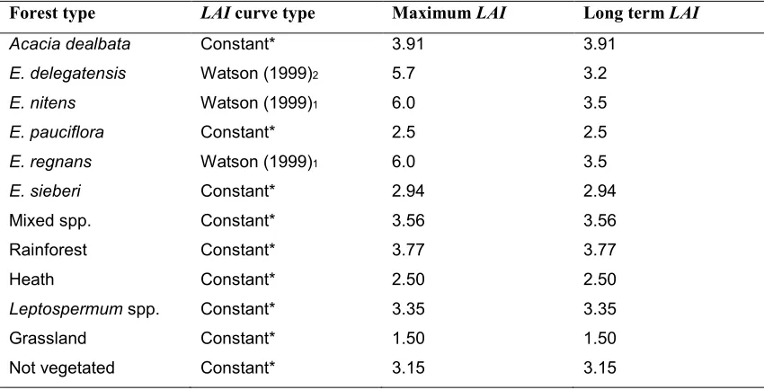
2.1: LAI:Age curve types and long-term trends in LAI for main vegetation types in Melbourne’s water catchments (from Feikema et al., 2006). P19.

2.2: Summary of catchment area and percentage of ash vegetation in the study areas. P25.

2.3: Weighted average long term rainfall and pan evaporation, calculated wetness index, and relative wetness index of the study catchment relative to the Maroondah catchments (from Feikema et al., 2006). P26.

2.4: Summary of the percentage of acceptable EUS’s for each catchment (from Feikema et al., 2006). P31.

4.1: Summary statistics of permanent plots exposed to a range of silvicultural treatments. P99.

4.2: Summary statistics of the extended plots located in six 1939 regenerating forest catchments exposed to a range of silvicultural treatments. P99.

4.3: Flight details and sensor configurations for the LiDAR data acquisition. P101.

4.4: List of stream gauges used in the study and the forest age over the duration of the hydrological time series. P102.

4.5: List of (a) North Maroondah and (b) Coranderrk rain stations used in the study, and the elevation of each station as well as the duration and length of each dataset.P104.

5.1: Continuous distribution functions implemented using the GAMLSS package (from Stasinopoulos et al., 2008). P114.

5.2 List of plot level LiDAR indices generate for each plot. P118.

5.3: Best performing distribution functions for plot-based LiDAR evaluated in this study. P123.

5.4: The four best performing distribution functions for each plot extent in each catchment and the number of plots that performed the best for a given mixture model in a given catchment. Empty records imply that the plot size is the same as the original plot size for the given catchment. P124.

5.5: RMSE and R2 of the ridge regression model, as well as the list of predictor variables used in the final model to predict eucalyptus: (a) basal area, and (b) stand volume, for each catchment and all catchments lumped together. Predictor variables with an astricts symbol (*) were developed by stratifying the vegetation layers using mixture models. P129.

5.6: RMSE and R2 of ridge regression models using only predictor variables that do not require mixture modelling (i.e. rows 1, 2, 3, 10, and 15 in table 5.2). 130.

5.7: RMSE and R2 of ridge regression used to predict non eucalyptus basal area and the list of predictor variables in the final model. P131.

6.1: Summary ofthe random effects for the final model structure, with 95% confidence intervals of the variance-covariance structure for each catchment in the study. P159.

(19)

7.1: Climate Filter Models for Myrtle 1 Catchment. P184.

7.2: Climate Filter Models for Slip Catchment. P184.

7.3: Improvements in the standard error of residuals when compared to the climate filter used by Kuczera (1987). P185.

8.1: Summary statistics of stand characteristics using ridge regression models. Catchments are stratified into stream buffer, hillslope, and treated areas. Coded stand characteristics in table include: Non (non-eucalypt), Euc (eucalypt), BA (basal area), and Vol (stand volume). P218.

(20)

List of Symbols, Variables, and Units

Age Age of the forest years

BA Basal area m2 ha-1

CAI Current annual increment m2 ha-1 yr-1

DBH diameter at breast height cm

ETp Pasture evapotranspiration m yr-1

ETf Forest evapotranspiration m yr-1

ET Evapotranspiration m yr-1

Eo annual potential evapotranspiration m yr-1

ε light-use efficiency g MJ-1

gs max maximum stomatal conductance cm s-1

gs stomatal conductance cm sec-1

gc canopy conductance cm sec-1

G Above ground productivity m3 ha-1yr-1 k Sapwood hydraulic conductivity m3 m-2sec-1

Lmax maximum reduction in average streamflow yield mm

LA Leaf area m2

LAI Leaf area index m2(leaf) m2(ground)

MAI Mean annual increment m2 ha-1 yr-1

P Precipitation mm

Pmax Maximum forest growth increment m3 ha-1yr-1

Q Solar Radiation µ mol m-2 sec-1

Qa Canopy absorbed radiation µ mol m-2 sec-1

Qt Observed runoff m3 day-1

q Sap flux density mL cm-2 hr-1

Rn net radiation W m-2

Rj Stem resistance Pa hr-1 kg-1

_{stomatal resistance} _sec-1 _cm-1

∆S changes in soil water storage J m-2 day-1

SA Sapwood area m2

(21)

t Temperature oC

T Transpiration m yr-1

Tmaxsf time of maximum yield reduction years Tmaxsf time of maximum forest growth rates years

VPD Vapour Pressure Deficit Pa

w plant available water capacity -

wf forest available water capacity - wp pasture available water capacity -

W Soil moisture mm

∆W Soil water deficit mm

WUE Water use efficiency m3 (stem) m-3 (water)

ψmax Pre-dawn leaf water potential Pa

ψl Leaf water potential Pa

(22)

1

Chapter 1: Introduction

1.1. Context and background of the water resource issue

Forest disturbance caused by timber harvesting or bushfire processes leads to changes in structure and density of natural forests, which causes changes in

evapotranspiration (ET) and hence streamflow over the regeneration period. After the 1939 bushfires in mountain ash forest (E.regnans) of Melbourne’s water catchments, a relationship between forest age and streamflow yield was found to suggest that regenerating forests use more water than mature forest (Langford, 1976).

Experimental studies of these findings have been confirmed with a large body of research identifying the causal processes (Kuczera, 1987; Vertessy et al., 1993; Vertessy et al., 1996; Watson, 1999; Watson et al., 1999a; Vertessy et al., 2001; Watson et al., 2001; Feikema et al., 2006; Pfautsch et al., 2010).

Forested catchments of south-eastern Australia are very dynamic ecosystems regularly subject to land cover disturbance. In recent history, Victoria has had 1.12 million ha burn in 2002/03; 1.15 million ha burn in 2006/07; and an area 30% of Melbourne’s water catchments burn in 2008/09. In 1939, an area of almost 2 million ha burnt in Victoria, whereas in Tasmania only 265,000 ha burnt in 1967. The intensity of the burns over these regions has been highly variable, which effectively resulted in highly variable regeneration processes and hence post-disturbance ET

rates. As well as bushfire disturbances, management of State Forests in both Tasmania and Victoria involves a range of silvicultural practices that harvest vast regions of timber-producing land with 60 to 100 years logging rotations. The scale of natural and anthropogenic land cover disturbance in forested catchments is having a significant effect on future streamflow trends.

In Australia, important water supply catchments are often largely forested,

(23)

2 Despite this, no study has developed a generalised approach for accurate assessment of how broad-scale changes in forest structure influence ET. This substantial

knowledge gap imposes serious limitations on our ability to predict future water availability from forested catchments.

1.2. Managing regenerating forest water use

Kuczera (1987) generalised the relationship between forest age and streamflow using rainfall and runoff data from eight forested catchments subject to the 1939 bushfire, and the resulting model is cited as the well-known “Kuczera Curve” shown in figure 1.1. The Kuczera Curve shows that two years after an old-growth forest disturbance, annual streamflow average begins to decrease and reaches its lowest value for forests 27 years of age, before a gradual recovery to pre-disturbance streamflow levels when the forest reaches maturity. In the 1990s, Victorian forest management agencies predicted the effects of planned forestry operations in Ash type forests of

Melbourne’s water catchments using the Kuczera curve and forest age data, without accounting for forest water use variation due to other environmental influences (Watson, 1999).

Figure 1.1: The Kuczera Curve (with 90% confidence limits) predicting water yield decline from

forest age in Mountain ash forests. Minimum yield is predicted to occur when the forest is 27 years

old

In recognising the inaccuracies in streamflow predictions that assume spatial

(24)

3 water resource subject to planned forestry operations and bushfire disturbance in Victoria (Feikema et al., 2006). Macaque consists of more than 70 parameters, and quantifies spatiotemporal changes in ET using data from E.regnans forest to empirically derive a canopy Leaf Area Index (LAI) versus age relationship, and stomatal conductivity (gs) versus age relationship.

For Macaque’s ET estimates to be data-driven with site-specific information, extensive measurements of LAI and gs within and above the canopy are required. Unfortunately, quantifying gs of E.regnans is difficult due to their great heights (>65m), and calculations of LAI is complicated by the vertical orientation of

E.regnans leaves (England & Attiwill, 2006) and line-of-site obstruction by understorey vegetation. There are also challenges in measuring seasonal and inter-annual variability of LAI due to site-specific effects of water deficit on leaf

production rates, expansion rates, size, senescence and shedding. For these reasons, spatiotemporal estimates of LAI and gsare highly uncertain and strongly influenced by the site-specific conditions during and prior to data collection.

Applying Macaque to forest types other than E.regnans is also inaccurate as the model does not empirically quantify forest water use in non-ash and mixed-species forest. Even though there is evidence that similar, although subdued, responses to land-cover disturbance occur in such forests (Cornish, 1993; Cornish & Vertessy, 2001; Lane & Mackay, 2001; Roberts et al., 2001; Bren et al., 2010; Macfarlane et al., 2010), Macaque assumes non-ash forest types have a constant water use

equivalent to old-growth conditions. The challenges in measuring spatiotemporal changes in LAI and gs has meant Macaque has been applied across vast regions of Victoria and Tasmania with empirical data for E.regnans forest from small site-specific experiments, and assumptions for non-ash forest types known to be unreliable. As Macaque also requires site-specific information on catchment level understorey LAI and gs, similar challenges also exist in quantifying spatiotemporal changes in understorey ET rates.

Dynamic forested catchments that supply water for downstream communities consist of a range of forest types and age classes, transpiring at different rates and

(25)

4 reason, it is necessary to quantify the impact of vegetation dynamics on the water

resource so that decision makers, planners, and managers of the forested water resource optimise drought security with appropriate restrictions, allocations, and deliveries of water resource.

1.3. The need for a data-driven model framework

Forest hydrology models in south-eastern Australia would benefit greatly from a data-driven methodology that quantifies hydrologically related plant physiological processes to explain spatiotemporal forest water use with site- and species-specific information. This dissertation aims to address this significant limitation in forest hydrology by developing forest growth models that quantify hydrologically relevant forest regeneration processes. It is argued that present forest hydrology models, used for policy applications in south-eastern Australia, undermine the importance of existing forest inventory and forest mensuration databases for managing the forested water resource. Detailed forest inventory data exists for most catchments in south-eastern Australia, and this information needs to be used more effectively to manage future streamflow trends.

Using typical forest inventory data, this dissertation quantifies spatiotemporal stand volumes and stand basal area (BA) for a set of stream gauged catchments, as both of these forest characteristics represent hydrologically relevant changes in regeneration processes. For example, Kuczera (1987) chose the gamma equation to represent decadal streamflow trends as the non-linear curve was considered to reflect changes in forest growth rates. Generally speaking, eucalyptus growth rates are the inverse of the Kuczera curve along the time axis as forest growth curves have an initial rapid increase in growth rates followed by a gradual reduction in growth rates after a maximum growth rate is reached. The present dissertation is the first published study that uses forest inventory data to produce forest growth models to explain streamflow trends in hydrological time series.

(26)

5 becomes more economically viable to harvest the timber and regenerate a faster growing forest. Tasmania’s and Victoria’s sustainable timber yield calculations determine the harvesting rotations, and hence forest age and water use over State forests, with no explicit scientific evaluation (except for Melbourne’s water catchments) to determine appropriate restrictive measures on the rate of disturbance in order to account for

catchment-specific water resource demand (Forestry Tasmania, 2007; Vanclay & Brack, 2008). Using forest inventory data in forest hydrology models allows for water use to be integrated into forest agency data management systems. Such an approach would allow for relevant policy makers to create integrated catchment management policies with data-driven models that are able to quantify streamflow for environmental and societal needs once the effects of bushfire disturbance or timber harvesting is accounted for.

Over the past two decades, a large body of forest hydrology research has scaled up tree-level water use to the catchment-level using sap flow measurements (Dunn & Connor, 1993; Vertessy et al., 1995; Haydon et al., 1996; Vertessy et al., 1997; Forrester et al., 2009; Macfarlane et al., 2010; Pfautsch et al., 2010). The research suggests differences in ET with age are overwhelmingly a result of differences in stand sapwood conducting area (SA). As BA is a good predictor of SA (Vertessy et al., 1997), accurate spatiotemporal BA estimates over forested catchments provides site- and species-specific information for explaining spatiotemporal forest water use. For this purpose, the present study produces a novel methodology for generating high resolution spatiotemporal BA estimates across large regional landscapes.

1.3. Research questions

The following research questions are addressed in this dissertation:

1. In Victoria and Tasmania, are existing forest hydrology models data-driven with vegetation dynamics that affect forest water use?

2. Does plant physiological theory support the use forest growth models to explain forest water use?

(27)

6 4. Can climate filters be used to remove the climatic variability in streamflow in

order to quantify a decadal streamflow trend attributed to forest regeneration processes?

5. Can forest inventory data be used to generate spatiotemporal forest growth models to explain streamflow trends in hydrological time series during the regeneration period of a timber producing forest?

1.4. Aims

The overarching aims of this dissertation are to:

• Use readily available forest inventory data to quantify the forest regeneration process with forest characteristics useful for forest hydrology research.

• Develop a climate filter that removes climatic variability in streamflow, and undertake a simulation exercise that determines how parameter inference is affected by data availability of the hydrological time series and the extent of the land-cover disturbance.

• Demonstrate that spatiotemporal forest growth models may be used to

explain catchment-level trends in forest water use over the forest regeneration period.

1.5. Thesis outline

Chapter two reviews Tasmania’s and Victoria’s forest hydrology models used to inform policy makers of the potential impacts of land cover disturbance on the water resource. The review provides a critique on how existing models represent the forest regeneration processes that influence forest water use.

Chapter three reviews plant physiological characteristics that regulate the soil-to-atmosphere water flow pathway of timber yielding forest types and plantations, with the overall objective to identify the processes that affect spatiotemporal variability in forest water use. The review also explores the relationship between plant

physiological regulators of forest productivity and water use, to provide scientific reasoning for using forest inventory data to explain decadal streamflow trends.

(28)

7 description of the study site, field measurements, forest inventory data, and

hydrological time series is also presented.

Chapter five uses Light Detection and Ranging (LiDAR) data to produce a generalised approach for stratifying and characterising the structure of specific vegetation layers of a multilayered eucalyptus forest over a catchment. The methodology produces canopy profile indices of understorey and overstorey vegetation using mixture models with a wide range of theoretical distribution functions. The methodology is applied to permanent plot data to predict overstorey stand volumes and basal area, and understorey basal area of mountain ash forest.

Chapter six applies permanent plot data to mixed effects models to estimate the spatial heterogeneity and temporally polymorphic nature in forest growth over the catchments. Using both the logistic and gamma equations, parameter estimates of the forest growth models were determined for each catchment.

Chapter seven applies aggregated rainfall data to the climate filter sub-model of the overall model structure to explain the climatic variation in the hydrological time-series data. A simulation exercise is undertaken to determine: how the climate filter parameter inference is affected by the extent and duration of the hydrological time series; and how substantial a post-disturbance decadal streamflow trend needs to be for the model structure to accurately identify it.

Chapter eight spatially distributes the forest growth models to generate lumped to the catchment forest growth curves for evaluation against the modelled trends in

streamflow data. The limitations of the present study are also discussed and recommendations for future research are presented.

(29)

8

Chapter 2: Review of Tasmania’s and Victoria’s forest

hydrology models

2.1. Introduction

This chapter provides a review of forest hydrology models, Macaque and

TasLUCaS; both of which are designed to quantify impacts of land cover disturbance on streamflow in Victoria and Tasmania respectively. A review of model

applications that address State level policy obligations is also undertaken to

determine whether forest and water resource managers are provided with an accurate assessment of how forest harvesting and other land cover disturbances affect

community water supply. First, an overview of the Kuczera curve is presented, as the Kuczera curve has contributed significantly to the development of both models, and hence overall management of forested water resource in both States.

2.2. Kuczera curve

In 1939 a bushfire burnt a large portion of Melbourne’s water-supply catchments resulting in significantly reduced streamflow during the following decades.

Approximately 53% of Melbourne’s water supply catchments are fire sensitive ash-type species (i.e. E.regnans, E.delegatensis and E.nitens) that were extensively and irreversibly damaged by the fires. The rest comprise of fire resistant drier mixed-species (i.e. E.obliqua and E.viminalis) that survived the fires with thick fire-resistant bark and epicormic shoots to replace the scorched crown. Kuczera (1985) analysed data from eight catchments affected by the 1939 bush fire to develop a model that estimated reductions in average catchment streamflow below old-growth forest streamflow levels. In the study, Kuczera (1985) assumed there was no impact of burnt mixed species forest on long-term streamflow trends as mixed species survive fire.

The effect of natural variations in climate poses a fundamental problem in detecting long-term streamflow trends during regeneration, and to describe this variation Kuczera (1987) used Langford’s (1976) climate-index model. This involved

(30)

9 pre-disturbance streamflow records; and by subtracting the effects of climate indices from post-fire streamflow records the residuals represent streamflow changes due to forest regeneration. Langford’s (1976) methodology required three assumptions: (1) a moderate to long term pre-fire streamflow record (ten or more years) to calibrate the climate-index model; (2) the pre-fire streamflow data needed to represent old-growth forest unaffected by earlier fires; and (3) pre-fire vegetation needed to be killed and regenerating over most of the catchment to identify a trend.

Kuczera (1987) was able to relax the first two assumptions by replacing Langford’s linear regression technique with a non-linear curve that was consistent with available evidence on long-term streamflow recovery. The assumed recovery recognised streamflow reductions are largely explained by post-disturbance forest growth rates, and as growth rates of mature or old-growth ash are very small, pre-disturbance streamflow in old-growth catchments is almost stationary with a quasi hydrologic equilibrium. Figure 2.1 shows the general shape of the long-term streamflow trend curve, which is consistent with available evidence on stand growth rates (West & Mattay, 1993). The exact shape of the post-disturbance streamflow trend curve was a priori unknown and regression theory, with least squares error assumptions, was used on streamflow data to infer posterior distributions and confidence limits of hydrologic parameters. These parameters included maximum reduction in average yield (Lmax) and time to maximum yield reduction (1/K) following bushfire.

Figure 2.1: The Gamma curve used by Kuczera (1985) to represent vegetation-induced reduction in

(31)

10 The results found that all eight catchments attained their maximum streamflow reduction relative to old growth forest about 20-30 years after disturbance. No significant streamflow increases were evident immediately after the disturbance. The resulting fits were satisfactory with goodness of fit criteria R2 ranging between 0.77 and 0.9. Kuczera (1987) regionalised the model outcomes using an empirical Bayes approach to relate the estimated hydrologic parameters to measured catchment characteristics such as forest composition. It was concluded that for a catchment with 100% regenerating ash forest with pre-disturbance annual streamflow of 1100 mm, the regional model estimated a maximum yield reduction of 615 mm approximately 27 years after disturbance, as shown in the Kuczera curve of figure 1.1.

2.3. Macaque: Victoria’s forest hydrology model

The Kuczera curve is a useful representation of the potential impacts of land cover disturbance on the water resource but the challenge lies in extrapolating the curve so that it is useful for a broader range of environmental conditions. For this purpose, Watson (1999) developed a process based model that evaluates the effects of land cover disturbance on streamflow with adjustable parameters based on site specific conditions. The Macaque model (Watson 1999) simulates temporal streamflow predictions quantified by Kuczera (1985) by hypothesising catchment water yield changes could be explained by changes in Leaf Area Index (LAI) and stomatal conductance (gs). The model operates at a daily time-step to simulate predictions

over 100 years and focuses on large-scale forest hydrological processes.

Macaque contains over 70 parameters and although there are dozens of parameters to calibrate, in practice most are given default values and calibration involves two parameters; the precipitation scalar to adjust the rainfall surface (water input), and the ratio of hydraulic gradient to the surface gradient to control the internal drainage rate (transfer function). The present critique of Macaque focuses on three modelling components that quantify changes in ET with forest age. These are: (1) canopy LAI

(32)

11

2.3.1. Ash eucalypt canopy LAI versus age relationship

The central component in Macaque is the representation of the canopy LAI versus age relationship (LAI:Age curve), which was produced with a set of allometric relationships illustrated in the flow chart of figure 2.2. The first step involved an allometric model relating destructive measurements of LA of 78 individual E.regnans

trees from four stands, with measured tree diameter at breast height (DBH) and mean

DBH for the trees in the stand to which the tree belonged too. In the second step, the allometric model was applied to a database of 2079 DBH measurements from 17

E.regnans stands in order to derived LAI predictions for each stand. Thirdly, the 17 stand LAI predictions where plotted against stand age and adjusted for variations in stocking rates to produce the LAI:Age curve. An evaluation of the regressions used to construct the LAI:Age curve is presented in the next section.

Figure 2.2: Flow chart summarising the steps taken to establish the relationship between LAI and age

(from Watson, 1999)

Step 1

Step 2

[image:32.595.178.533.350.656.2]

(33)

12

2.3.1.1. Calculation of ln(LA) versus ln (DBH) and mean ln(DBH)

(Step 1)

Data from four single aged stands, aged 5, 16, 56, and 225 years old were used to predict LA from DBH and mean DBH of an E.regnans forest stand. Figure 2.3 plots tree LA versus DBH along the log-log axis showing clustering of data for each stand as well as the sample mean (white circle) of each stand (Watson et al., 1999a). The linear regression lines for the 5, 16, 56, and 225 year old stands in figure 2.3 have an

[image:33.595.165.454.263.484.2]

R2 of 0.898, 0.929, 0.836, and 0.085 respectively.

Figure 2.3: Sample LA versus DBH for four stands plotted on the log axis, which also provides;

regression lines, sample means (white circles) and population means (grey circles) estimated from simple regression equations outlined below (from Watson, 1999).

2.3.1.2. Calculation of mean stand LA versus mean and standard

deviation of ln(DBH) (Step 2)

In order to predict stand LA with the tree-level relationship in figure 2.3, each stand’s sample mean and population mean of DBH was required. This complicated the situation as the LA data was not always measured in conjunction with the DBH

measurements of all trees in the stand population. For this reason, population mean

(34)

13 that regeneration does not take place until sometime after age zero. In maximising

R2, the calibrated adjustment of 5.04 was higher than expected for the hypothesised delay in forest development. Thus, Watson (1999a) acknowledges the model is not reliable at predicting mean DBH for forests younger than or close to five years of age.

(a)

[image:34.595.164.459.174.527.2]

(b)

Figure 2.4: Logarithmic plot with the line of best fit for (a) exp-mean-In DBH versus ages, and (b)

exp-mean-In DBH versus adjusted ages (from Watson, 1999).

As the regression in figure 2.4(b) uses a dataset different to the one used to construct the LAI versus DBH relationship in figure 2.3, it was necessary to assume the

sampled values of ln(DBH) from the 17 stands were uniformly distributed in order to allow for LAI estimates of these stands. Figure 2.5 provides standardised ln(DBH)

(35)

14

Figure 2.5: Histograms (using lines instead of bars) of ln(DBH) values within each stand;

standardised and scaled to have zero mean, unit standard deviation, and unit area. A standard normal probability distribution function is provided for reference (from Watson, 1999).

To derive stand ln(LA), the population means of ln(DBH) at age 5, 16, 56, and 225 was used even though figure 2.3 shows a clear offset between each stand’s sample (white circle) and population mean (grey dot); indicating the LA samples were not representative of the stand populations with a bias towards sampling larger trees (Watson et al., 1999a). Using this estimated population mean of ln(DBH), figure 2.6(a) shows the linear regression between mean stand ln(LA) and mean stand

ln(DBH). In figure 2.6(a), the 225 year old stand represents a population mean derived from a LA sample with R2of 0.085, whereas the five year old stand with BA

estimates was considered dubious as a result of the required adjustment undertaken in figure 2.4. Using the relationship in figure 2.6(a), the final model for predicting LA

(36)

15

(a)

(b)

Figure 2.6 (a) Estimated variation in (estimated) population mean between stands ln(LA) and

ln(DBH) and; (b)LA versus DBH for the four stands with 95% confidence limits (dashed lines) (from Watson, 1999).

2.3.1.3. Constructing the LAI

versus age relationship (Step 3)

The LAI:Age relationship was constructed using the 17 stands with DBH

measurements and the model predicting LA, which meant mean LA for trees within each stand needed to be derived. As shown in the flow chart of figure 2.2, the procedure required an estimation of the variance of ln(DBH) with the assumption that the distribution of DBH for all stands had a normal distribution. However, figure 2.5 shows the distributions were actually irregular, multimodal, and peaked. Figure 2.7 shows the line of best fit for variance of ln(DBH) versus adjusted age; with an

[image:36.595.162.438.66.465.2]

(37)

16

Figure 2.7: Line of best fit for variance of In(DBH) versus age for each stand (from Watson, 1999).

The above assumptions and regression equations were then used to construct the

LAI:Age curve for the 17 forest stands. Results in figure 2.8(a) show a great deal of scatter, which was improved in Figure 2.8 (b), by correcting the relationship based on each stand’s deviation in stocking rates; even though the 17 stands were meant to represent healthy fully stocked single-aged E.regnans stands. The data used in the relationship represents fully stocked stands, which are rare in native forests and for this reason more scatter would be expected for typical forest stands found in catchments requiring forest hydrology management. The final E.regnansLAI:Age

(38)

17

(a)

(b)

Figure 2.8: Predicted LAI versus age for healthy, fully stocked single-aged stands (a) uncorrected, and

(b) corrected for variability in stocking rate and the final model is superimposed (from Watson, 1999).

It is important to recognise that the LAI:Age relationship relied on LA measurements of 78 individual trees from four stands. The methodology fails to recognise the seasonal and inter-annual variability of LAI due to site-specific effects of water deficit on leaf production rates, expansion rates, size, senescence, and shedding. For this reason, extrapolating the LAI model in space and time is full of uncertainty as measurements at one point in time were strongly influenced by the site-specific conditions during and prior to data collection.

2.3.2. Non-ash eucalypt and non eucalypt LAI versus age

relationship

[image:38.595.173.494.68.426.2]

(39)

18 in LAI for the first 5 to 10 years followed by a constant species-specific LAI, as shown in figure 2.9. The species-specific constant in table 2.1 was derived from areal average remotely sensed LAI values using the methodology described in section 2.3.3. For all non-ash species listed in table 2.1, the curve in figure 2.9 results in streamflow increase for the first 5-10 years after disturbance of old-growth, followed by a recovery to constant old-growth streamflow levels. These estimates are known to be incorrect as non-ash species follow a similar streamflow trend to ash-species (Cornish, 1993; Cornish & Vertessy, 2001; Lane & Mackay, 2001; Roberts et al., 2001; Macfarlane et al., 2010).

(40)

[image:40.595.128.553.106.323.2]

19

Table 2.1:LAI:Age curve types and long-term trends in LAI for main vegetation types in Melbourne’s

water catchments (from Feikema et al., 2006).

Forest type LAI curve type Maximum LAI Long term LAI

Acacia dealbata Constant* 3.91 3.91

E. delegatensis Watson (1999)2 5.7 3.2

E. nitens Watson (1999)1 6.0 3.5

E. pauciflora Constant* 2.5 2.5

E. regnans Watson (1999)1 6.0 3.5

E. sieberi Constant* 2.94 2.94

Mixed spp. Constant* 3.56 3.56

Rainforest Constant* 3.77 3.77

Heath Constant* 2.50 2.50

Leptospermum spp. Constant* 3.35 3.35

Grassland Constant* 1.50 1.50

Not vegetated Constant* 3.15 3.15

* Constant after first 5 to 10 years after establishment derived from remote sensed images; 1 Watson (1999), Equation 8.45; 2 Watson (1999), Equation 8.45. Same as 1 but with LAI lower by 0.3

2.3.3. Spatial distribution of LAI over the catchment

With the use of Landsat TM images from four different years, two attempts were made by Watson (1999) to extrapolate the LAI:Age curves and develop spatial maps of total LAI. Shade correctionswhere performed on the images to remove the effects of illumination and viewing angles. The shade-corrected images were used to

calculate the normalised difference vegetation index (NDVI), which recognises the positive correlation between vegetation amount and near infra-red reflectance, and the negative correlation between vegetation amount and red reflectance. The shade-corrected NDVI data were used to produce transformed NDVI (TNDVI) values, which did not improve results but converts the values into LAI estimates.

(41)

20 not vary greatly for vegetation between 20 and 240 years of age, raising uncertainty for LAI estimates using age specific NDVI maps.

Figure 2.10: 50 m radius-averaged NDVI derived from shade corrected imagery plotted against

ground measured LAI using a Li-Cor PCA (from Feikema et al., 2006).

Figure 2.11: The relation between shade-corrected NDVI and forest age for E.regnans (from Feikema

et al., 2006).