Doppler images and the underlying dynamo: the case of AF Leporis

A&A 574, A25 (2015)

DOI:10.1051/0004-6361/201424229 c

ESO 2015

Astronomy

&

Astrophysics

Doppler images and the underlying dynamo

,,

The case of AF Leporis

S. P. Järvinen

, R. Arlt

, T. Hackman

, S. C. Marsden

, M. Küker

, I. V. Ilyin

, S. V. Berdyugina

,

K. G. Strassmeier

, and I. A. Waite

1 _{Leibniz-Institut für Astrophysik Potsdam, An der Sternwarte 16, 14482 Potsdam, Germany} e-mail:sjarvinen@aip.de

2 _{Department of Physics, University of Helsinki, PO Box 64, 00014 Helsinki, Finland}

3 _{Finnish Centre for Astronomy with ESO (FINCA), University of Turku, Väisäläntie 20, 21500 Piikkiö, Finland}

4 _{Computational Engineering and Science Research Centre, University of Southern Queensland, 4350 Toowoomba, Australia} 5 _{Kiepenheuer-Institut für Sonnenphysik, Schöneckstr. 6, 79104 Freiburg, Germany}

Received 19 May 2014/Accepted 3 November 2014

ABSTRACT

Context.The (Zeeman-)Doppler imaging studies of solar-type stars very often reveal large high-latitude spots. This also includes F stars that possess relatively shallow convection zones, indicating that the dynamo operating in these stars differs from the solar dynamo.

Aims.We aim to determine whether mean-field dynamo models of late-F type dwarf stars can reproduce the surface features recovered in Doppler maps. In particular, we wish to test whether the models can reproduce the high-latitude spots observed on some F dwarfs. Methods.The photometric inversions and the surface temperature maps of AF Lep were obtained using the Occamian-approach inversion technique. Low signal-to-noise spectroscopic data were improved by applying the least-squares deconvolution method. The locations of strong magnetic flux in the stellar tachocline as well as the surface fields obtained from mean-field dynamo solutions were compared with the observed surface temperature maps.

Results.The photometric record of AF Lep reveals both long- and short-term variability. However, the current data set is too short for cycle-length estimates. From the photometry, we have determined the rotation period of the star to be 0.9660±0.0023 days. The surface temperature maps show a dominant, but evolving, high-latitude (around+65◦) spot. Detailed study of the photometry reveals that sometimes the spot coverage varies only marginally over a long time, and at other times it varies rapidly. Of a suite of dynamo models, the model with a radiative interior rotating as fast as the convection zone at the equator delivered the highest compatibility with the obtained Doppler images.

Key words.stars: imaging – stars: activity – starspots – stars: individual: AF Leb – dynamo

1. Introduction

Solar-type stars form a very broad class of stars from late-F to early-K type dwarfs and sub-giants, all containing a con-vective envelope over a radiative interior. Observations of these stars provide excellent constraints for theoretical dynamo mod-els. Our understanding of the operation of the magnetic dynamo in such stars is based on the solar case, where the solar activ-ity cycle is believed to be generated through dynamo action op-erating either in the convection zone or in the stably stratified layer beneath it (for a short overview of solar dynamo models see, e.g.,Passos et al. 2014). One would expect stars with an internal structure similar to that of the Sun, that is, stars with convective envelopes, to show the same type of dynamo oper-ation. However, (Zeeman-)Doppler imaging studies frequently

_{Partially based on observations made with the Nordic Optical}

Telescope, operated by the Nordic Optical Telescope Scientific Association at the Observatorio del Roque de los Muchachos, La Palma, Spain, of the Instituto de Astrofísica de Canarias.

_{Based partly on STELLA SES data.}

_{Tables 1–3 and Figs. 7–14 are available in electronic form at}

http://www.aanda.org

find large spots at high latitudes and large regions of a near-surface azimuthal field (not seen on the solar near-surface). For very active stars, it has been suggested that instead of a solar-like dy-namo, which probably works in the overshoot zone, a distributed α2_{Ω- orα}2_{-dynamo is likely to be present (Brandenburg et al.}

1989;Moss et al. 1995).

F stars possess relatively shallow convection zones. Nevertheless, observations show via the Doppler imaging method that at least some of these stars have high-latitude and even polar spots (e.g., AF Lep:Marsden et al. 2006;τBoo:Fares et al. 2009; one of the components in σ2 CrB: Strassmeier & Rice 2003). Furthermore, surface differential-rotation estimates imply thatδΩ increases with decreasing depth of the convec-tion zone (e.g., Marsden et al. 2011b; Barnes et al. 2005a). Theoretical models support this result (e.g.,Küker & Rüdiger 2007).

AF Lep (HR 1817, HD 35850) is an active, young, rapidly rotating, single solar-like star. The first photometric observa-tions of the target are from the late 60s (Stokes 1972), and it was also detected with EXOSAT (Cutispoto et al. 1991). It has been identified as a member of the β Pictoris moving group, which has been estimated to have an age of ∼20 Myr

(Fernández et al. 2008and references therein;Binks & Jeffries 2014;Mamajek & Bell 2014). The colours suggest a spectral classification of F8/9 (Cutispoto et al. 1996). The high Li abun-dance (logN(Li)=3.2), solar metallicity, and high rotation ve-locity (vsini = 50 km s−1_{) are consistent with the star being}

a young object. Furthermore, it has an unusually high intrinsic X-ray luminosity of∼1.6×1030_{ergs s}−1_{for a single, late-F-type}

star (Tagliaferri et al. 1994).

The first photometric monitoring of the star by Cutispoto et al.(1996) did not reveal photometric variability. However, the flat-bottomed shapes of StokesIline intensity profiles suggested that a dark spot is present on AF Lep (Budding et al. 2002). Later, a photometric follow-up revealed a prominent photomet-ric minimum in a phase diagram (Budding et al. 2003).

This paper has two parts. In the first part, we explore what we can learn about AF Lep via photometric and spectroscopic observations. The second part of the paper consists of theoretical calculations aiming to determine whether high-latitude spots can be formed.

2. Observations and data reduction

2.1. Photometric observations

We started to observe AF Lep in March/April 2010 with the

Amadeus, a T7 Automatic Photoelectric Telescope (APT) at

Fairborn Observatory, jointly operated by the University of Vienna and Leibniz-Institute für Astrophysik Potsdam (AIP), with Johnson-CousinsVfilter (for more details seeStrassmeier et al. 1997b). After that, four additional data sets were obtained (see Fig. 1). During the first observing run the star was ob-served from four to nine times per night for a month. The sub-sequent runs lasted longer – from four to five months – but the star was observed less frequently, and there are only one or two data points per night. Measurements were made differentially between the target, a comparison star (HD 36379), a check star (HD 34538), and the sky position. The data reduction is au-tomated and was described by Strassmeier et al. (1997a) and Granzer et al.(2001a).

2.2. Spectroscopic and spectropolarimetric observations

Most of the spectroscopic and spectropolarimetric observa-tions of AF Lep were carried out during two simultaneous ob-serving runs with the fibre-fed STELLA Echelle Spectrograph (SES) mounted on STELLA-I (Tenerife; Strassmeier et al. 2004;Granzer et al. 2001b) and the Anglo-Australian Telescope (AAT) with the SEMPOL visiting polarimeter (Semel et al. 1993; Marsden et al. 2011a) during December 2008 and November/December 2009. The STELLA observations were also continued into January 2010. Furthermore, AF Lep had been observed earlier in November 2005 with SOFIN at the Nordic Optical Telescope (NOT, La Palma). The STELLA data have a continuous wavelength coverage (3900–9000 Å) with a resolving power of 55 000. The spectra from the AAT have a shorter wavelength coverage (4380–6810 Å) but higher resolu-tion (∼70 000). The SOFIN échelle spectrograph, acquired with the second camera, provides 33 useful orders in a spectral range of 3930–9040 Å. The slit width of 65μm centred at 6427 Å gives a resolution of 76 000. More information is presented in Tables1–3.

5500 6000 6500 6.30

6.25 6.20 6.15 6.10

5500 6000 6500 HJD +2450000

6.30 6.25 6.20 6.15 6.10

V magnitude

2010 2011 2012 2013 2014 Year

a

1970 1980 1990 2000 2010 Year

6.35 6.30 6.25 6.20 6.15

V magnitude

b

Fig. 1.a)V-band photometric data of AF Lep with measurement errors used in this paper. The mean value of each observing season is plotted with redx.b)The whole photometric record in theV-band: the blue arrowhead represents data fromStokes(1972), the red asterisks data

fromCutispoto et al.(1996), the green bar illustrates the magnitude

range fromBudding et al.(2003), and black dots represent this work.

3. Determining the rotation period

As summarised bySilva-Valio(2008), for example, there are two methods that are used to determine a rotation period of a star. One uses rotational broadening of spectral lines. This method, however, is usable only for stars that rotate faster than a thresh-old velocity set by the spectral resolution and has always sini un-certainty,ibeing the inclination of a star. Furthermore, it gives an average of the periods of the whole stellar disk. The other method uses the periodic modulation of the stellar flux due to the co-rotating dark and bright features on the stellar surface. The advantages of this method are that it can also be used for stars with long periods, it is only mildly affected by latitudinal differential rotation, and the obtained period corresponds to the period of the latitudes where these features are. However, nor-mally, the information on the latitudes of stellar active regions cannot be extracted from a one-dimensional data set, that is, a light-curve. Lately, starspot detections during planetary transits are also used for estimating rotation periods that represent peri-ods at specific latitudes (seeSilva-Valio 2008).

mixture of cool spots and bright faculae that evolve on different timescales. However, in very active stars, the cool spots prob-ably dominate the variation. And not only that, but the optical variability of the Sun is dominated by several active regions at the same time. One has to keep in mind that sunspots and solar active regions have typical lifetimes of days to weeks (Solanki 2003), whereas starspots have been observed to persist over a long time (e.g.,Strassmeier 2009).

Co-rotating spots on the surface, pulsations, spot evolution, instrumental effects, and a combination of all of them can intro-duce periodic variations in the light curves. Despite these effects, light curves often show notable stability in the phase, shape, and amplitude of photometric variability over long times.Meibom et al.(2011) discussed the two possible explanations for this: ei-ther the spots are longer-lived than the sunspots, or they tend to emerge non-uniformly at preferred long-lived active longitudes. The outcome from the first scenario was that although on the Sun the lifetime of the spots increases linearly with area, and the so-lar log-normal spot distribution is strongly dominated by small spots, there is no evidence that the log-normal distribution holds for other stars. However, on other stars the small spots domi-nate as well, although they are very often unresolved (see, e.g., Lanza et al. 2009; Silva-Valio et al. 2010). Furthermore, life-times of individual starspots can be short (Mosser et al. 2009), but the large-scale spot groups can live long (Hussain 2002). The second possibility was that starspots emerge at preferred longi-tudes. Here it is assumed that the spots seen in photometry and in Doppler images are not huge individual spots, but rather spot groups consisting of a range of smaller spots emerging at pre-ferred longitudes. This could lead to obtaining observed spotted-ness over longer periods of time although individual spots come and go. AsMeibom et al.(2011) stated, the only requirement is that the emergence rate is high enough to maintain a rather stable spot coverage, but this is expected for young and active stars.

The rotation period of AF Lep has commonly been reported to be around one day:Budding et al.(2003) usedP = 1d._{0 for}

phasing photometry andMarsden et al.(2006) reported a period of∼1d._{0 from spectroscopy. This is notoriously near the typical}

window of ground observations (P0 = 0d.9972), which creates

challenges for determining the period from ground-based pho-tometry. To achieve a good phase coverage using a single tele-scope, observations covering a long time-base are needed, which in turn may mean that the surface features (and thus the light curve) have undergone significant changes during this time. We can also expect significant problems with spurious periods very near the real one.

We applied time-series analysis methods to the March/April 2010 photometry set (Fig.1a). Using the Lomb method for un-evenly sampled data (Press et al. 1992), we detected a promi-nent double peak corresponding to periods of 0d._{97 and 1}d_.03

(Fig.2). Using the method described by Jetsu & Pelt (1999), we estimated that the probability of 1d._{03 being a real period was}

4×10−6_{, while 0}d_{.97 passed the test of being non-spurious. This}

method uses bootstrapping for the model parameter error esti-mates, evaluates the modelling statistics with the Kolmogorov-Smirnov test, and identifies spurious periodicities from real ones with the phase residual regression. We then applied the continuous-period search method (Lehtinen et al. 2011), which accounts for changing spot patterns, using a window length (ΔTmax) covering the whole data set. In practice, this meant

fit-ting the model ycps(ti,β¯)=a0+

K

k₌1

akcos (2πk f ti)+bksin (2πk f ti) (1)

0.5 1.0 1.5 2.0

0 10 20 30 40

0.5 1.0 1.5 2.0

Period [d] 0

10 20 30 40

Power

0.97 1.03

1.21

1.48

Fig. 2. Lomb-periodogram showing possible rotation periods.

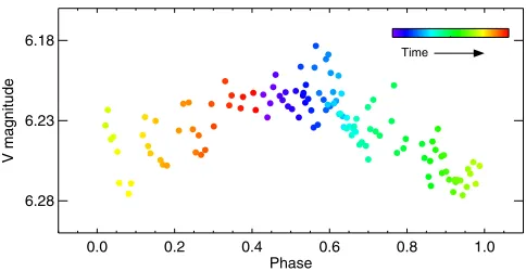
0.0 0.2 0.4 0.6 0.8 1.0 Phase

6.28 6.23 6.18

V magnitude

Time

Fig. 3. Phase diagram for the periodPphot =0.9660 using the March/ April 2010 data set. The observations cover 30 days and the data points have been colour-coded with increasing time of observations.

to the observations (y). Herea0,ak,bkand f = 1/Pphotare free

parameters and ti the times of the observations. With the

op-timal orderK = 1, we obtained the period Pphot ≈ 0d.9660±

0d._{0023 and the time of the first photometric minimum HJD} 0 =

2 455 268.227±0.039. Thus we used the ephemeris

HJDmin=2 455 268.227+0.9660E, (2)

to derive the rotation phases for our photometric and spectro-scopic data. The phase diagram using this ephemeris for the March/April 2010 photometry is displayed in Fig.3.

4. Photometric variability

0 90 180 270 360 −90 0 90 2010.17 a)

0.0 0.2 0.4 0.6 0.8 1.0 Phase 6.33

6.21

6.10 _31d

0 90 180 270 360 −90

0 90

2010.75 b)

0.0 0.2 0.4 0.6 0.8 1.0 Phase 6.33

6.21 6.10

50d

0 90 180 270 360 −90

0 90

2010.83 c)

0.0 0.2 0.4 0.6 0.8 1.0 Phase 6.33

6.21 6.10

28d

0 90 180 270 360 −90

0 90

2010.92 d)

0.0 0.2 0.4 0.6 0.8 1.0 Phase 6.33

6.21

6.10 _17d

0 90 180 270 360 −90

0 90

2011.00 e)

0.0 0.2 0.4 0.6 0.8 1.0 Phase 6.33

6.21

6.10 _26d

0 90 180 270 360 −90

0 90

2011.75 f)

0.0 0.2 0.4 0.6 0.8 1.0 Phase 6.33

6.21 6.10

36d

0 90 180 270 360 −90

0 90

2011.92 g)

0.0 0.2 0.4 0.6 0.8 1.0 Phase 6.33

6.21 6.10

46d

0 90 180 270 360 −90

0 90

2012.08 h)

0.0 0.2 0.4 0.6 0.8 1.0 Phase 6.33

6.21

6.10 _44d

0 90 180 270 360 −90

0 90

2013.75 i)

0.0 0.2 0.4 0.6 0.8 1.0 Phase 6.33

6.21

6.10 _41d

0 90 180 270 360 −90

0 90

2014.00 j)

0.0 0.2 0.4 0.6 0.8 1.0 Phase 6.33

6.21 6.10

23d

1.0 0.8 0.6 0.4 0.2 0.0 Spot filling factor

Fig. 4. Each data subset (a–j) is visualised with two images. The given times represent the middle point of each set.On the left, we show the light-curve inversion result. The spot-filling factor is larger in the darker regions. A light curve represents a one-dimensional time series and, therefore, the resulting stellar image contains information on the spot distribution only in longitudinal direction.On the right, the observed and calculatedV-band magnitudes are plotted with crosses and lines, respectively. The length of the set (in days) is given in the upper right corner.

is not long enough to obtain a reliable cycle length estimate. However, a local minimum occurred around mid-2011, a local maximum was reached around 2012/2013, and in early 2014 the star was dimmer again. Furthermore, the amplitude of the bright-ness variations implies rotational modulation due to changing spot coverage.

To analyse the short-term variability in detail, we inverted the light curves into stellar images (for details about the method, seeBerdyugina et al. 2002). As seen from Figs.3and4a, from March/April 2010 it is possible to obtain a smooth light curve, where the data points from the beginning of the observing sea-son match those obtained at the end of the seasea-son with the obtained period. However, the amplitude of the night-to-night variations is relatively large. In this subset, the spots are con-centrated around phaseϕ = 0.0. However, the second data set (August 2010–January 2011), shows significant short-term vari-ations and can be divided into four subsets (Figs.4b–e). These sets show moderate phase migration, and a secondary minimum appears in the light curves (Figs.4b–d). A new subset was started when a clear change in the photometric behaviour was detected, that is, a real break in the observations, or when the subse-quent data points started to form a maximum instead of a min-imum. Variability is also present in later data sets, although ob-servations are rather infrequent and, therefore, it is not always possible to create a continuous light curve over all phases (see Fig.4g), where observations covering 46 days have large scatter and a gap of 0.4 in phase. The photometric minimum is often rather broad, which agrees with high-latitude spots (see Sect.5) and the inclination of the star.

The drifting of the spot longitudes aroundϕ = 0.0 may be due to an error in the period, which is not easy to determine in this case, as discussed in Sect. 3. An alternative explana-tion might be a significant surface differential rotation. Using Zeeman-Doppler imaging with StokesV-profiles,Marsden et al. (2006) derived values of Ωeq = 6.495±0.011 rad d−1 and

δΩ =0.259±0.019 rad d−1_{for AF Lep. The third option might}

be drifting due to an azimuthal dynamo wave (Cole et al. 2014),

although we recall that it is a competitive mechanism to the dif-ferential rotation, and the drift could be due to a combination of them.

5. Surface spot configuration

The spectroscopic observations were phased with the derived new ephemeris (Eq. (2)). Local line profiles were calculated with the code of Berdyugina (1991). This includes calculating the opacities in the continuum and in atomic and molecular lines, although in this paper molecular lines were omitted. Atomic line parameters were obtained from the Vienna Atomic Line Database (VALD;Piskunov et al. 1995;Kupka et al. 1999). The stellar model atmospheres used here are fromKurucz(1993). The local line profiles were calculated for 20 values ofμ=cosθ from the disk centre to the limb. The spectra were calculated for temperatures ranging from 4000 K to 6500 K in steps of 250 K. The Occamian approach was used to invert of the observed line profiles into stellar images (Berdyugina 1998). A 6◦×6◦ grid on the stellar surface was used to integrate local line profiles into normalised flux profiles. With a set of stellar atmosphere models, the stellar image is considered as the distribution of the effective temperature across the stellar surface, as is commonly done in Doppler imaging. This code does not take differential rotation into account. The stellar parameters used are presented in Table4.

The noise in both STELLA and AAT data was reduced us-ing the least-squares deconvolution (LSD) technique (seeSemel 1989andDonati et al. 1997for the algorithm; andJärvinen & Berdyugina 2010for the application). For this purpose, a line mask containing 93 spectral lines was built using lines within a wavelength range of 4770–6900 Å. They are mainly Fe

i

i

i

2008.95

Phase = 0.0 Phase = 0.25 Phase = 0.5 Phase = 0.75 Pole−on

4449 4747 5044 5342 5639 5937 6234 6532 T, [K]

4942− 6223−

2009.92

Phase = 0.0 Phase = 0.25 Phase = 0.5 Phase = 0.75 Pole−on

4449 4747 5044 5342 5639 5937 6234 6532 T, [K]

4509− 6187−

Fig. 5.Temperature maps of AF Lep from the data sets with a good phase coverage. They were obtained by combining simultaneous AAT and STELLA observations. For both seasons the map is shown from four angles and pole-on. The used phases have been marked with ticks around the pole-on projection. All maps have a common temperature scale, and the highest and lowest temperature of each map is shown at the left side of the temperature scale.

2005.87

Phase = 0.0 Phase = 0.25 Phase = 0.5 Phase = 0.75 Pole−on

4449 4747 5044 5342 5639 5937 6234 6532 T, [K]

4449− 6531−

2010.04

Phase = 0.0 Phase = 0.25 Phase = 0.5 Phase = 0.75 Pole−on

4449 4747 5044 5342 5639 5937 6234 6532 T, [K]

4594− 6328−

Fig. 6.Temperature maps of AF Lep from the data sets with an incomplete phase coverage. The 2005 data set was obtained at the NOT, the 2010 data set with STELLA. Otherwise maps as in Fig.5.

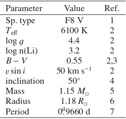
Table 4.Stellar parameters of AF Lep with references.

Parameter Value Ref.

Sp. type F8 V 1

Teff 6100 K 2

logg 4.4 2

log n(Li) 3.2 2

B−V 0.55 2,3

vsini 50 km s−1 2 inclination 50◦ 4

Mass 1.15M 5

Radius 1.18R 6

Period 0d._{9660 d 7}

References. (1) Eggen (1986); (2) Tagliaferri et al. (1994);

(3)Cutispoto et al. (1996); (4) Marsden et al. (2006); (5) Kim &

Demarque(1996); (6)Blackwell & Lynas-Gray(1994); (7) this work.

The resulting temperature maps are shown in Figs.5and6. The fits to the observed spectra and LSD profiles are shown in Figs.7–10and the differences between the mean profile and the observed ones are illustrated in Figs.11–14to visualise spots

moving through the line profiles. To create the temperature map from 2005 observations, all available individual SOFIN obser-vations were used. For the other temperature maps, mainly the SEMPOL spectra from the AAT were used because it gives the best phase coverage, and the long phase-gaps were filled using the STELLA spectra. For the spectropolarimetric SEMPOL ob-servations there are four consecutive StokesIexposures for each StokesV exposure that were added together. The photospheric temperature of 6200 K agrees with earlier results and the spec-tral type of the star. A cool spot is located near the polar region of the star. The time separation of the maps in Fig.5is one year. Although the total spot coverage has seemingly changed very little, clear evolution is detected. In the first map (2008.95) the spot is formed from two components atϕ = 0.77 (secondary) and atϕ=0.96 (primary). In the latter map (2009.92), the spot has grown larger and the two components now have equal sizes and form a larger spot that covers half of the polar longitudes. The middle point is atϕ=0.47 and the spot is also cooler. The mean latitude of the spot is around+65◦.

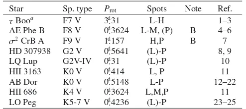
Table 5.Overview of spot latitudes in comparable targets sorted ac-cording to the spectral type of the stars.

Star Sp. type Prot Spots Note Ref.

τBooa _{F7 V 3}d_{.31 L-H 1–3}

AE Phe B F8 V 0d._{3624 L-M, (P) B 4–6}

σ2_{CrB A F9 V 1}d_{.157 H,P B 7}

HD 307938 G2 V 0d._{5641 (L)-P 8, 9}

LQ Lup G2V-IV 0d._{31 (L)-P 10}

HII 3163 K0 V 0d._{414 L, P 11}

AB Dor K0 V 0d._{5148 L-P 12–22}

HII 686 K4 V 0d._{3624 L,M,P 11}

LO Peg K5-7 V 0d._{4236 (L)-P 23–25}

Notes.In the “Spots” column P=polar, H=high-latitude, M= mid-latitude, and L=low-latitude. Parenthesis around the letter are used when spots are not always present in that latitude range or are weak. The binarity is stated in the “Note” column with “B”.(a)_Only Zeeman-Doppler imaging maps, no brightness, spot occupancy, nor temperature maps.

References. (1) Catala et al. (2007); (2) Donati et al. (2008);

(3) Fares et al. (2009); (4) Maceroni et al. (1991); (5) Maceroni

et al.(1994); (6)Barnes et al.(2004); (7)Strassmeier & Rice(2003);

(8) Marsden et al. (2004); (9) Marsden et al. (2005); (10) Donati

et al. (2000); (11) Stout-Batalha & Vogt (1999); (12)Kürster et al.

(1994); (13)Collier-Cameron & Unruh(1994); (14)Collier Cameron

(1995); (15)Unruh et al.(1995); (16)Hussain et al.(1997); (17)Unruh

& Collier Cameron(1997); (18) Donati & Collier Cameron (1997);

(19) Donati et al. (1999); (20) Collier Cameron et al. (1999);

(21)Donati et al.(2003); (22)Jeffers et al. (2007); (23)Lister et al.

(1999); (24)Barnes et al.(2005b); (25)Piluso et al.(2008).

phasesϕ = 0.11–0.55. In the 2005.87 map the main feature is atϕ = 0.00 with a tail, which has a mid-point atϕ = 0.18. In the 2010.04 map the spot is again smaller with the mean phase ofϕ=0.35. This map also has the lowest spot latitude (+61◦). However, when taking into account the spatial resolution of the maps, the mean latitude of the spots remains relatively constant. The maps inverted from the data with an incomplete phase cov-erage have a broader temperature range than the maps inverted from the data with a good phase coverage.

The high-latitude spot is anti-symmetric around the polar re-gion in all the maps, and there are no low-latitude features. In this sense the maps presented here differ from the (∼2002.00) map byMarsden et al.(2006), which shows a very compact po-lar (completely above latitude+75◦) spot and some very weak low-latitude features.

To validate the obtained results, the spot configuration on AF Lep should be compared with spot configurations on other F dwarfs and with spot configurations on other fast-rotating (P ≤ 1 d) dwarfs. Unfortunately, there are not many F dwarfs that have been mapped to date. A short overview of the current knowledge about the spot configuration in comparable stars is presented in Table5. Some binary components are included as well, although they do not make good comparisons because they are very different entities. More comparison targets can be found in an extensive list ofStrassmeier(2009).

High-latitude spots are thus common features in rapidly ro-tating dwarfs, and sometimes the maps show the whole polar re-gion to be covered with spots. A more interesting aspect than how these high-latitude/polar spots can be formed would be whether low-latitude spots are detected or not. However, we re-call that the maps have been made and visualised using diff er-ent techniques. Therefore, it is difficult to judge how prominer-ent the low-latitude features are. Furthermore, low-latitude features

6706.1 6706.8 6707.5 6708.1 6708.8 6709

0.88 0.90 0.92 0.94 0.96 0.98 1.00

Lithium

6706.1 6706.8 6707.5 6708.1 6708.8 6709

Wavelength [Å] 0.88

0.90 0.92 0.94 0.96 0.98 1.00

Normalized flux

Fig. 15.Mean lithium-line profiles for the 2008 (red) and 2010 (blue) observations. For comparison, we have plotted synthetic spectra calcu-lated using logN(Li)=3.25 (dotted line) and logN(Li)=3.35 (dashed line), assuming a fixed temperature in the model calculations.

appear often less resolved as a result of lower spatial resolution. The simulations show that the places of the spots (or spot groups) are correct, but the temperature contrast suffers from the lack of resolution.

6. Lithium abundance

Tagliaferri et al. (1994) have reported a lithium abundance of logN(Li)=3.2 for AF Lep. Our 2005 observations do not cover the lithium line, but for the later observations this region is cov-ered. We determined the lithium-line equivalent width for all individual spectra listed in Tables1 and 2. To do this, we fit-ted a double Gaussian to the Li

i

i

Generally, during 2008 the equivalent width of the lithium line was measured to be smaller than in 2009 or 2010. A clear dif-ference is seen in the mean lithium-line profiles (Fig.15). As expected (see, e.g.,Pallavicini et al. 1993;Cutispoto 2002), the seasonal equivalent-width variations do not show any clear cor-relation with the phases of the spots. An excellent review of the relationship between spots and lithium equivalent width varia-tions is given byFekel(1996).

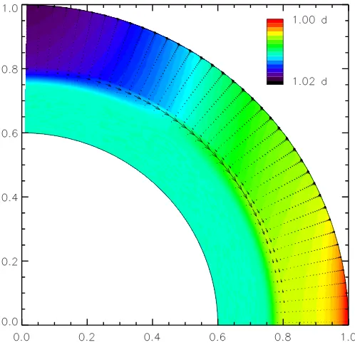
Fig. 16.Rotation profile and meridional circulation from theΛ-effect model in the vertical cross-section of the computational domain, as-suming that the core rotation is the average angular velocity between equator and pole at the bottom of the convection zone. Note that the shear layer near 0.8R_∗is not an artefact but the result of theΛ-effect model.

obtained byMentuch et al.(2008) andWeise et al.(2010) are in between,EW =146 mÅ andEW =149 mÅ, respectively. The mean profile of the 2008 observations has an equivalent width of 160 mÅ, while the corresponding value from 2010 mean pro-file is 182 mÅ.

7. Dynamo solutions

7.1. Dynamo setup

The aim of this section is to use the theoretical results for the differential rotation and meridional circulation computed for a star of 1.2 Min a kinematic dynamo model to study whether we can produce a theoretical butterfly diagram that is compara-ble with the observed spot locations. We chose a spherical shell withr,θ, andφ being the radius, colatitude, and azimuth, and placed the inner boundary at 60% of the stellar radiusR_∗(which is well within the radiative interior of a late-F star), while the outer radius is the stellar surface. The velocity is a vector fieldu, constant in time, containing the theoretical differential rotation and meridional circulation of the star (see, e.g., Fig.16). They were obtained independently from a mean-field hydrodynamic model employing theΛ-effect and the baroclinicity emerging in rotating, stratified turbulence (Rüdiger 1989; Küker et al. 1993; Kitchatinov et al. 1994; Kitchatinov & Rüdiger 2005). A comparison of a large set of differential rotation parameters obtained for low-mass stars from theKeplermission (Reinhold et al. 2013) and the theoretical predictions by theΛ-effect the-ory (Küker & Rüdiger 2011) shows a fair agreement and gives us confidence in applying the method to a particular, observed star.

The other effect of rotating, stratified turbulence is the α-effect, which gives rise to a turbulent (averaged) electromotive force, generating poloidal magnetic fields from toroidal ones,

and vice versa (Krause & Rädler 1980). The existence of this net effect has been debated recently and may require the removal of small-scale magnetic helicity from the stellar convection zone (Blackman & Brandenburg 2003;Warnecke et al. 2011). We did not consider the exterior here and assumed that it grants the ex-istence of theα-effect.

We solved the induction equation in the mean-field formula-tion with anα-effect,

∂B ∂t = ∇ ×

u×B+α(r, θ,B2)◦B−1

2(∇ηT)×B

−∇ ×ηT∇ ×B, (3)

whereBis the large-scale magnetic field andu is a given ve-locity field. The equation also includes diamagnetic pumping, which is a result of a gradient in the turbulent velocities and of-ten neglected in mean-field dynamos. Whenever a gradient in the turbulent magnetic diffusivityηTis implemented, a variation

of the turbulence intensity is implied and requires treatment of the diamagnetic pumping (Krause & Rädler 1980;Kitchatinov & Olemskoy 2012).

The radius of the starR∗ andηT are used to normalise the

induction equation, which then modifies to ∂_Bˆ

∂t = ∇ ×

C_Ωuˆ×Bˆ +Cαψ( ˆB2)αˆ(ˆr, θ)◦Bˆ −1

2(∇ηˆT)×Bˆ

−∇ ×ηˆT∇ ×Bˆ, (4)

where we also split the α-tensor into a spatially varying part and a part depending onB2, since they are (assumed to be) in-dependent. The resulting dimensionless parameters areC_Ω = R2_∗Ωeq/ηTandCα=R∗α0/ηT, withΩeqbeing the equatorial

sur-face angular velocity andα0 the maximumα-effect in the star

in m/s.

For better legibility, we omit all hats from the normalised quantities ofr,u,B,α, andηin the following. In general,αis a tensor of which ourα-term contains the symmetric part, while the antisymmetric part is represented by the diamagnetic pump-ing term, with all three distinct elements of the latter bepump-ing equal to−∇η/2. The six distinct tensor elements ofαfor fast rotation (anisotropicα-effect) are

αrr = f(r) cosθ(1−2 cos2θ),

αθθ = f(r) cosθ(1−2 sin2θ), αφφ= f(r) cosθ,

αrθ=2f(r) cos2θsinθ, and αrφ=αθφ=0;

f(r)= 1

2

1+erf

_r−r

cz

d , (5)

wherercz =0.8 is the bottom radius of the convection zone and d=0.02 is the thickness of the transition to the radiative interior, motivated by the results for the solar tachocline (e.g.,Antia & Basu 2011). The convection-zone thickness is based on a stellar model of a 1.2MZAMS star with solar metallicity, computed with the MESA stellar evolution code (Paxton et al. 2011). The quenching functionψ(B2_{) represents the suppression of the}

tur-bulence by large-scale magnetic fields (Brandenburg et al. 1989), that is, the strength of theα-effect, and is defined as

ψ(B2)= 1 1+B2_/B2

eq

Fig. 17.Modified rotation profile with an interior rotating as fast as the bottom of the convection zone at the equator. The meridional circulation is the same as in Fig.16.

The magnetic field at which theα-effect drops significantly is the equipartition field strength,Beq= √μ0ρurms, whereμ0is the

permeability constant,ρthe gas density, andurmsthe

root-mean-square convective velocity.

The magnetic diffusivity in the radiative interior is much lower than the turbulent diffusivity in the convection zone. We employ an arbitrary function for the non-dimensional diffusivity,

ηT=ηcore+

ηcz−ηcore

2

1+erf

_r−r

cz

d , (7)

whereηcore=0.01 is the diffusivity in the interior andηcz =1 is

the turbulent value in the convection zone.

AssumingR_∗ = 1.1 R,P =1.0 days, and a turbulent dif-fusivity ofηT = 1012 cm2/s, we obtain a magnetic Reynolds

number ofC_Ω = 4.09×105_{. The meridional flow obtained in}

conjunction with the differential rotation isum =48 m/s, giving

a flow Reynolds number of 363.1.

The bottom boundary conditions at r = 0.6 for the mag-netic field correspond to perfect conductor conditions, while the top boundary at r = 1 has exactly vacuum conditions. The mean-field induction Eq. (4) is solved with the numerical code byHollerbach(2000). As already indicated, we read the veloc-ity field u = (ur(r, θ),uθ(r, θ),uφ(r, θ)) from the output of the

Λ-effect model for the convection zone. In the latter, the bound-ary conditions for the flow model were stress-free at the stel-lar surface and at the bottom of the convection zone. Note that this is not the bottom boundary of the dynamo model. Since the computational domain for the dynamo is larger, the differential rotation was extrapolated to sharply change to a uniform rota-tion in the radiative interior (as we know it does in the Sun). The choice of the rotation rate of the interior is free in principle, so we chose two cases: one takes theΩof mid-latitudes in the convection zone, the other uses the equatorialΩof the convec-tion zone. The theoretical rotaconvec-tion patternsΩ(r, θ) for AF Lep are illustrated in Figs.16and17.

7.2. Results

The minimumCαfor a growing antisymmetric (dipole-like) so-lution is 0.20, while it is 1.05 for the symmetric (quadrupole-like) solution. Since magnetic fields suppress the turbulence whence the α-effect (quenching), the effective α-effect is re-duced to its lowest marginal value in any place where fields grow. A symmetric solution is therefore very unlikely in AF Lep. We concentrate on antisymmetric solutions in the following. For the estimated magnetic Reynolds number ofC_Ω =4.09×105_,

both antisymetric and symmetric solutions are stationary. Strong meridional circulation can change the oscillatory behaviour of the solutions into stationary ones (Küker et al. 2001).

The latitudinal distribution of the azimuthal magnetic field at the tachocline and the radial field at the surface are plotted over time in Fig.18. The plot for the tachocline fields is mo-tivated by the concept that the strong shear at the base of the convection zone generates strong azimuthal fields that eventu-ally become buoyantly unstable and rise to the surface to form spots (not modelled here). The largest tachocline fields reside at low latitudes. With this location, high-emergence latitudes are extremely difficult to achieve, since thin flux-tube simu-lations do not show tubes emerging at axis distances smaller than the starting distance (Granzer et al. 2000). The highest emergence latitudebefor a given initial latitudebiis therefore

cosbe = rczcosbi. An initial latitude (residence of strong

dy-namo fields) of 30◦results in a highest emergence latitude of 46◦. The largest azimuthal fields ofBmax_φ = 5.5 occur atr = 0.75 because of the pumping, which is most efficient on stationary fields. The strongest radial surface fields are also constrained to latitudes below about 40◦. We do not believe the observed high-latitude fields can be explained with this dynamo solution.

Using an isotropic α-effect withαrr = αθθ = αφφ

(corre-sponding to very slow rotation unlike AF Lep), we also obtain stationary solutions with an unchanged criticalCα =0.20. The Ω-effect is just much stronger in the toroidal-field equation than any of the variousα-components.

The magnetic diffusivity is a relatively poorly known value in the bulk of the convection zones of the Sun and stars. We computed the dynamo solutions for two other values ofηT, 1011

and 1013cm2/s, leading toCΩ = 4.09×106(LoEta) andCΩ = 4.09×104_{(HiEta), respectively. These diffusivities correspond to}

diffusion times of 1900 yr and 19 yr, again usingR_∗as the length scale. The ratio between rotational and meridional velocity is al-ways kept the same. The LoEta run delivers a stationary solution as well, with a criticalCα =0.43. The HiEta run leads to an os-cillatory solution with a criticalCα=10.8 – a strongerα-effect is now needed to compensate for the weakerΩ-effect. The butter-fly diagram shows significant azimuthal fields at the tachocline and radial surface fields only below 60◦latitude (Fig.19).

Fig. 18.Butterfly diagram for the solution with diamagnetic pumping and maximum anisotropy inαaccording to (5).Left: azimuthal magnetic fieldBφat a radius of 0.8R∗(maximum valueBmaxφ =0.52);right: radial fieldBrat the stellar surface (maximum valueBmaxr =0.0007).

Fig. 19.As in Fig.18, but for a magnetic diffusivity ten times higher. Maximum values areBmax

φ =0.052 (left) andBmaxr =0.0095 (right).

Fig. 20.As in Fig.18, but with a fast-rotating interior (roughly equatorial surface rotation). Maximum values areBmax

φ =0.76 (left) andBmaxr =

0.044 (right).

If the value for the magnetic diffusivity is correct, the period of the cycles in Fig.20would be 4.5 yr. A possible cycle period of about 4 yr is indicated by the upper panel of Fig.1(see also Sect.4), resulting in a full-cycle period of 8 yr including a field reversal. Given our ignorance of the exact turbulent magnetic diffusivity, the model cycle time is compatible with the observed long-term variability.

An alternative approach to the solar dynamo is the flux-transport dynamo, which is based on the Babcock-Leighton

0.2 0.4 0.6 0.8 1.0 1.2 DIFFUSION TIMES

-50 0 50

LATITUDE

-0.1 Beq

0.1 Beq

0.00 0.05 0.10 0.15

DIFFUSION TIMES -50

0 50

LATITUDE

-0.1 Beq

0.1 Beq

Fig. 21.Butterfly diagram for the solution with diamagnetic pumping, Babcock-Leighton-type source term for the poloidal magnetic field, and a turbulent magnetic diffusivityηT=1012cm2/s.Left: classical solar case with a poloidal-field generation by active regions at low latitudes.Right: observationally driven case with a poloidal-field generation around 70◦ latitudes. In both cases the toroidal magnetic field at the bottom of the convection zone is plotted because this is the field relevant for spots in the Babcock-Leighton scenario.

0.20 0.21 0.22 0.23

DIFFUSION TIMES -50

0 50

LATITUDE

-3.1 Beq

3.1 Beq

0.20 0.21 0.22 0.23

DIFFUSION TIMES -50

0 50

LATITUDE

-5.2 Beq

5.2 Beq

Fig. 22.Babcock-Leighton-type dynamo solutions with the same setup as in Fig.21, but for the low turbulent magnetic diffusivityηT=1011cm2/s.

Left: classical solar case with a poloidal-field generation by active regions at low latitudes.Right: observationally driven case with a poloidal-field generation around 70◦latitudes.

typically used in the solar case, and a distribution motivated by the presence of spots on AF Lep near 70◦latitude. Theα-term now reads

Cαψ(B2φ(rcz, θ))α(r, θ)◦B(rcz, θ) (8)

and theα-components need to be replaced byαrr =αθθ=αrθ=

0 and αφφ = 1

2

1+erf

_r−r

s

d cosθsin

2_{θ, (solar case)}

αφφ = 1 2

1+erf

_r−r

s

d cosθsin

2 _θ−π

2

2.5

, (AF Lep)

wherers=0.95 restricts the poloidal-field production to a

near-surface layer. These are purely geometrical descriptions; the only physical requirement is the anti-symmetry about the equa-tor, achieved by cosθ, as was also used in the third line of Eq. (5). The main change is, however, the non-locality of this “α”-effect because it refers to the azimuthal field at the bottom of the con-vection zone, but acts at the surface. In contrast to solar flux-transport models, we did not restrictαφφto low latitudes, since this restriction is motivated by the low emergence latitudes of sunspots, which does not hold here.

When employing the turbulent magnetic diffusivity ofηT =

1012_cm2_{/s as used in the distributed-αdynamos above, we}

ob-tain stationary solutions, as shown in Fig.21. In both cases, the solar-type and the high-latitude Babcock-Leighton effect, the so-lutions are confined to low latitudes. We omit the surface radial-field plot here, since the mechanism relies on active regions forming as the result of rising flux from the toroidal field at the base of the convection zone.

A second ingredient to a Babcock-Leighton dynamo is a rel-atively low ηT. Figure 22 therefore shows the solutions for a

value ten times lower (LoEta), resulting inC_Ω = 4.09×106_.

The solutions are now oscillatory. The solar case shows naturally low-latitude fields, but the high-latitude case also exhibits large toroidal fields at low latitudes, because the meridional circula-tion, which is equatorward at the base of the convection zone, has a stronger impact on the solutions at this low value ofηT.

0.11 0.12 0.13 0.14 DIFFUSION TIMES

-50 0 50

LATITUDE

-2.4 Beq

2.4 Beq

0.11 0.12 0.13 0.14

DIFFUSION TIMES -50

0 50

LATITUDE

-2.4 Beq

2.4 Beq

Fig. 23.Babcock-Leighton-type dynamo solutions with the same setup as in Fig.22, but for a fast radiation zone. Again,left: poloidal-field generation at low latitudes, andright: poloidal-field generation around 70◦latitudes.

a clear activity pattern not higher than 40◦, even for a purely ax-ial flux rise, which is not simulated here.

The various dynamo solutions presented here favour a dis-tributed dynamo in the rapidly rotating convection zone of AF Lep, which gives results close to the observed spot lati-tudes if the radiative interior rotates as fast as the near-equator convection zone (unlike the solar radiation zone). We recall that the ZDI maps byMarsden et al.(2006) show regions of a near-surface azimuthal field, which also points to a distributed dynamo.

8. Summary and discussion

We have analysed both photometric and spectroscopic observa-tions of the young active F dwarf AF Lep and studied whether the obtained results can be explained with theoretical models.

The long-term photometric record of AF Lep, which cov-ers over 40 years of infrequent observations, shows that the star has become brighter over this time. While the whole pe-riod is not sufficiently sampled, the last 4.5 yr of observations are well covered and indicate a cyclic variation. The previously reported rotation period of∼one day implied that finding the true period from ground-based observations is challenging, es-pecially when the photometry also reveals short-term variability due to spot evolution and/or differential rotation. The photomet-ric light curves indicate that the spot coverage can remain sta-ble for months and then undergo several changes from month to month. With time-series analysis methods we have determined the rotation period to be 0.9660±0.0023 days.

Multi-site spectroscopic observations were used to recon-struct surface temperature maps that all show a dominant high-latitude spot. This indicates that the dynamo operating in this shallow convection zone star must differ from that of the Sun. The mean longitude of the spots drifts with time, but the latitude remains relatively constant (within the accuracy of the tempera-ture maps).

The lithium line of AF Lep shows some variability over the years. Because of the resolution (250 K) of the model calcu-lations we cannot rule out that the variations are simply due to overall temperature fluctuations. A fluctuating Li abundance seems quite unlikely. Our results, as well as the results from others, have shown that the equivalent width of the lithium line keeps changing. However, the seasonal variations of individual equivalent-width measurements do not show any clear correla-tion with the phases of the spots.

We considered various dynamo solutions to produce a the-oretical butterfly diagram that is comparable with the observed spot locations. A dynamo model based on a differential rotation profile in which the stellar interior rotates at the average surface angular velocity is not able to reproduce the high-latitude spots observed on AF Lep and also on other F dwarfs. However, if the stellar interior rotates with the same speed as the convection zone at the equator, it is possible to generate a substantial magnetic field at high latitudes of about 60◦. Such fast internal rotation may be compatible with the young age of AF Lep. The reader is also referred to a complementary study on a more slowly rotat-ing F-star recently published byBonanno et al.(2014).

It is rather common that ZDI maps of the stars show the magnetic flux spread over a wide range of latitudes. Over the years, the maps have started to show more and more complex field topologies, and increasingly weaker field strengths are de-tected as well.Strassmeier et al. (2013) compared independent magnetic maps made by two codes from almost simultaneous observations (seeSkelly et al. 2010andCarroll et al. 2012). The disparity of the two reconstructions is noticeable. As stated by Strassmeier et al.(2013), one can only speculate about the rea-sons for the differences. Clearly more comparisons of the codes are needed and all reconstructions have to be interpreted with care.

Acknowledgements. This work has made use of the VALD database, operated at Uppsala University, the Institute of Astronomy RAS in Moscow, and the University of Vienna. The authors thank the anonymous referee for useful and enlightening comments and suggestions.

References

Antia, H. M., & Basu, S. 2011, ApJ, 735, L45

Barnes, J. R., Lister, T. A., Hilditch, R. W., & Collier Cameron, A. 2004, MNRAS, 348, 1321

Barnes, J. R., Collier Cameron, A., Donati, J.-F., et al. 2005a, MNRAS, 357, L1 Barnes, J. R., Collier Cameron, A., Lister, T. A., Pointer, G. R., & Still, M. D.

2005b, MNRAS, 356, 1501

Berdyugina, S. V. 1991, Bull. Crimean Astrophys. Obs., 83, 89 Berdyugina, S. V. 1998, A&A, 338, 97

Berdyugina, S. V., Pelt, J., & Tuominen, I. 2002, A&A, 394, 505 Binks, A. S., & Jeffries, R. D. 2014, MNRAS, 438, L11 Blackman, E. G., & Brandenburg, A. 2003, ApJ, 584, L99 Blackwell, D. E., & Lynas-Gray, A. E. 1994, A&A, 282, 899 Bonanno, A., Fröhlich, H.-E., Karoff, C., et al. 2014, A&A, 569, A113 Brandenburg, A., Krause, F., Meinel, R., Moss, D., & Tuominen, I. 1989, A&A,

213, 411

Budding, E., Heckert, P., Soydugan, F., et al. 2003, Inform. Bull. Variable Stars, 5451, 1

Carroll, T. A., Strassmeier, K. G., Rice, J. B., & Künstler, A. 2012, A&A, 548, A95

Catala, C., Donati, J.-F., Shkolnik, E., Bohlender, D., & Alecian, E. 2007, MNRAS, 374, L42

Cole, E., Käpylä, P. J., Mantere, M. J., & Brandenburg, A. 2014, ApJ, 780, L22

Collier Cameron, A. 1995, MNRAS, 275, 534

Collier-Cameron, A., & Unruh, Y. C. 1994, MNRAS, 269, 814

Collier Cameron, A., Walter, F. M., Vilhu, O., et al. 1999, MNRAS, 308, 493 Cutispoto, G. 2002, Astron. Nachr., 323, 325

Cutispoto, G., Tagliaferri, G., Giommi, P., et al. 1991, A&AS, 87, 233 Cutispoto, G., Tagliaferri, G., Pallavicini, R., Pasquini, L., & Rodono, M. 1996,

A&AS, 115, 41

Donati, J.-F., & Collier Cameron, A. 1997, MNRAS, 291, 1

Donati, J.-F., Semel, M., Carter, B. D., Rees, D. E., & Collier Cameron, A. 1997, MNRAS, 291, 658

Donati, J.-F., Collier Cameron, A., Hussain, G. A. J., & Semel, M. 1999, MNRAS, 302, 437

Donati, J.-F., Mengel, M., Carter, B. D., et al. 2000, MNRAS, 316, 699 Donati, J.-F., Collier Cameron, A., Semel, M., et al. 2003, MNRAS, 345, 1145 Donati, J.-F., Moutou, C., Farès, R., et al. 2008, MNRAS, 385, 1179 Eggen, O. J. 1986, AJ, 92, 910

Fares, R., Donati, J.-F., Moutou, C., et al. 2009, MNRAS, 398, 1383

Fekel, F. C. 1996, in Stellar Surface Structure, eds. K. G. Strassmeier, & J. L. Linsky, IAU Symp., 176, 345

Fernández, D., Figueras, F., & Torra, J. 2008, A&A, 480, 735 Granzer, T. 2004, Astron. Nachr., 325, 417

Granzer, T., Schüssler, M., Caligari, P., & Strassmeier, K. G. 2000, A&A, 355, 1087

Granzer, T., Reegen, P., & Strassmeier, K. G. 2001a, Astron. Nachr., 322, 325 Granzer, T., Weber, M., & Strassmeier, K. G. 2001b, Astron. Nachr., 322, 295 Hollerbach, R. 2000, Int. J. Num. Meth. Fluids, 32, 773

Hussain, G. A. J. 2002, Astron. Nachr., 323, 349

Hussain, G. A. J., Unruh, Y. C., & Collier Cameron, A. 1997, MNRAS, 288, 343 Järvinen, S. P., & Berdyugina, S. V. 2010, A&A, 521, A86

Jeffers, S. V., Donati, J.-F., & Collier Cameron, A. 2007, MNRAS, 375, 567 Jetsu, L., & Pelt, J. 1999, A&AS, 139, 629

Kim, Y.-C., & Demarque, P. 1996, ApJ, 457, 340

Kitchatinov, L. L., & Olemskoy, S. V. 2012, Sol. Phys., 276, 3 Kitchatinov, L. L., & Rüdiger, G. 2005, Astron. Nachr., 326, 379 Kitchatinov, L. L., Ruediger, G., & Kueker, M. 1994, A&A, 292, 125 Krause, F., & Rädler, K. H. 1980, Mean-field magnetohydrodynamics and

dy-namo theory

Kürster, M., Schmitt, J. H. M. M., & Cutispoto, G. 1994, A&A, 289, 899 Küker, M., & Rüdiger, G. 2007, Astron. Nachr., 328, 1050

Küker, M., & Rüdiger, G. 2011, Astron. Nachr., 332, 933 Küker, M., Ruediger, G., & Kitchatinov, L. L. 1993, A&A, 279, L1 Küker, M., Rüdiger, G., & Schultz, M. 2001, A&A, 374, 301

Kupka, F., Piskunov, N., Ryabchikova, T. A., Stempels, H. C., & Weiss, W. W. 1999, A&AS, 138, 119

Kurucz, R. 1993, ATLAS9 Stellar Atmosphere Programs and 2 km s−1

grid. Kurucz CD-ROM No. 13. Cambridge, Mass.: Smithsonian Astrophysical Observatory, 13

Lanza, A. F. 2011, in IAU Symp. 273, eds. D. Prasad Choudhary, & K. G. Strassmeier, 89

Lanza, A. F., Pagano, I., Leto, G., et al. 2009, A&A, 493, 193

Lehtinen, J., Jetsu, L., Hackman, T., Kajatkari, P., & Henry, G. W. 2011, A&A, 527, A136

Lister, T. A., Collier Cameron, A., & Bartus, J. 1999, MNRAS, 307, 685 Maceroni, C., van’t Veer, F., & Vilhu, O. 1991, The Messenger, 66, 47 Maceroni, C., Vilhu, O., van’t Veer, F., & van Hamme, W. 1994, A&A, 288,

529

Mamajek, E. E., & Bell, C. P. M. 2014, MNRAS, 445, 2169

Marsden, S. C., Waite, I. A., Carter, B. D., & Donati, J.-F. 2004, Astron. Nachr., 325, 246

Marsden, S. C., Waite, I. A., Carter, B. D., & Donati, J.-F. 2005, MNRAS, 359, 711

Marsden, S. C., Mengel, M. W., Donati, F., et al. 2006, in ASP Conf. Ser. 358, eds. R. Casini, & B. W. Lites, 401

Marsden, S. C., Jardine, M. M., Ramírez Vélez, J. C., et al. 2011a, MNRAS, 413, 1922

Marsden, S. C., Jardine, M. M., Ramírez Vélez, J. C., et al. 2011b, MNRAS, 413, 1939

Meibom, S., Mathieu, R. D., Stassun, K. G., Liebesny, P., & Saar, S. H. 2011, ApJ, 733, 115

Mentuch, E., Brandeker, A., van Kerkwijk, M. H., Jayawardhana, R., & Hauschildt, P. H. 2008, ApJ, 689, 1127

Moss, D., Barker, D. M., Brandenburg, A., & Tuominen, I. 1995, A&A, 294, 155

Mosser, B., Baudin, F., Lanza, A. F., et al. 2009, A&A, 506, 245

Pallavicini, R., Cutispoto, G., Randich, S., & Gratton, R. 1993, A&A, 267, 145 Passos, D., Nandy, D., Hazra, S., & Lopes, I. 2014, A&A, 563, A18

Paxton, B., Bildsten, L., Dotter, A., et al. 2011, ApJS, 192, 3

Piluso, N., Lanza, A. F., Pagano, I., Lanzafame, A. C., & Donati, J.-F. 2008, MNRAS, 387, 237

Piskunov, N. E., Kupka, F., Ryabchikova, T. A., Weiss, W. W., & Jeffery, C. S. 1995, A&AS, 112, 525

Press, W. H., Teukolsky, S. A., Vetterling, W. T., & Flannery, B. P. 1992, Numerical recipes in Fortran, The art of scientific computing

Reinhold, T., Reiners, A., & Basri, G. 2013, A&A, 560, A4

Rüdiger, G. 1989, Differential rotation and stellar convection. Sun and the solar stars

Semel, M. 1989, A&A, 225, 456

Semel, M., Donati, J.-F., & Rees, D. E. 1993, A&A, 278, 231 Silva-Valio, A. 2008, ApJ, 683, L179

Silva-Valio, A., Lanza, A. F., Alonso, R., & Barge, P. 2010, A&A, 510, A25 Skelly, M. B., Donati, J.-F., Bouvier, J., et al. 2010, MNRAS, 403, 159 Solanki, S. K. 2003, A&ARv, 11, 153

Stokes, N. R. 1972, MNRAS, 159, 165

Stout-Batalha, N. M., & Vogt, S. S. 1999, ApJS, 123, 251 Strassmeier, K. G. 2009, A&ARv, 17, 251

Strassmeier, K. G., & Rice, J. B. 2003, A&A, 399, 315

Strassmeier, K. G., Bartus, J., Cutispoto, G., & Rodono, M. 1997a, A&AS, 125, 11

Strassmeier, K. G., Boyd, L. J., Epand, D. H., & Granzer, T. 1997b, PASP, 109, 697

Strassmeier, K. G., Granzer, T., Weber, M., et al. 2004, Astron. Nachr., 325, 527

Strassmeier, K. G., Carroll, T. A., Ilyin, I., & Järvinen, S. 2013, in IAU Symp. 294, eds. A. G. Kosovichev, E. de Gouveia Dal Pino, & Y. Yan, 447 Tagliaferri, G., Cutispoto, G., Pallavicini, R., Randich, S., & Pasquini, L. 1994,

A&A, 285, 272

Unruh, Y. C., & Collier Cameron, A. 1997, MNRAS, 290, L37

Unruh, Y. C., Collier Cameron, A., & Cutispoto, G. 1995, MNRAS, 277, 1145 Warnecke, J., Brandenburg, A., & Mitra, D. 2011, A&A, 534, A11

Weise, P., Launhardt, R., Setiawan, J., & Henning, T. 2010, A&A, 517, A88 White, R. J., Gabor, J. M., & Hillenbrand, L. A. 2007, AJ, 133, 2524 Wichmann, R., Schmitt, J. H. M. M., & Hubrig, S. 2003, A&A, 399, 983

Table 1.Spectroscopic observations of AF Lep with SES at the STELLA observatory.

HJD Day Phase S/N Exp.t HJD Day Phase S/N Exp.t

2 450 000+ s 2 450 000+ s

2008 5168.581883 03/12/2009 0.85 119 1200

4806.449041 05/12/2008 0.97 84 1200 5168.612782 03/12/2009 0.88 92 1200 4806.488960 05/12/2008 0.01 69 1200 5168.651441 03/12/2009 0.92 113 1200 4807.442635 06/12/2008 1.00 68 1144 5168.684299 03/12/2009 0.95 88 1200 4807.485140 06/12/2008 0.04 75 1200 5168.724356 03/12/2009 1.00 71 1200 4807.500198 06/12/2008 0.06 71 1200 5169.677176 04/12/2009 0.98 93 1200 4808.455330 07/12/2008 0.05 92 1200 5169.706822 04/12/2009 0.01 74 1200

4808.506302 07/12/2008 0.10 91 1200 2010

4808.686498 08/12/2008 0.29 95 1200 5210.375680 13/01/2010 0.11 107 1200 4809.455377 08/12/2008 0.08 91 1200 5210.481473 13/01/2010 0.22 113 1200 4809.514308 09/12/2008 0.14 79 1200 5210.510337 13/01/2010 0.25 113 1200

2009 5210.615744 14/01/2010 0.36 70 1200

5163.435205 27/11/2009 0.52 85 1200 5211.432112 14/01/2010 0.21 123 1200 5163.452347 27/11/2009 0.54 81 1200 5211.468481 14/01/2010 0.24 126 1200 5163.485338 27/11/2009 0.57 100 1200 5211.503232 14/01/2010 0.28 121 1200 5163.513160 28/11/2009 0.60 93 1200 5211.542212 15/01/2010 0.32 136 1200 5163.552318 28/11/2009 0.64 92 1200 5211.570609 15/01/2010 0.35 125 1200 5163.580713 28/11/2009 0.67 101 1200 5211.600474 15/01/2010 0.38 89 1200 5163.612288 28/11/2009 0.70 106 1200 5212.416273 15/01/2010 0.22 121 1200 5163.640174 28/11/2009 0.73 85 1200 5212.456635 15/01/2010 0.27 125 1200 5163.672249 28/11/2009 0.77 102 1200 5212.489709 15/01/2010 0.30 128 807 5163.700904 28/11/2009 0.79 90 1200 5212.566831 16/01/2010 0.38 133 1200 5163.736466 28/11/2009 0.83 63 1200 5212.606046 16/01/2010 0.42 97 1200 5164.503297 28/11/2009 0.63 94 1200 5213.412320 16/01/2010 0.26 99 1200 5164.640697 29/11/2009 0.77 86 1200 5213.455694 16/01/2010 0.30 116 1200 5164.674109 29/11/2009 0.80 106 1200 5213.499864 16/01/2010 0.35 103 1200 5165.457987 29/11/2009 0.61 90 1200 5213.541172 17/01/2010 0.39 109 1200 5165.499258 29/11/2009 0.66 97 1200 5213.569589 17/01/2010 0.42 119 1200 5165.529145 30/11/2009 0.69 99 1200 5214.413196 17/01/2010 0.29 91 1200 5165.568430 30/11/2009 0.73 93 1200 5214.450284 17/01/2010 0.33 92 1200 5165.596842 30/11/2009 0.76 76 1200 5214.484901 17/01/2010 0.37 100 1200 5165.625225 30/11/2009 0.79 99 1200 5214.513877 18/01/2010 0.40 97 1200 5165.652971 30/11/2009 0.82 92 1200 5214.561562 18/01/2010 0.45 80 1200 5165.680734 30/11/2009 0.84 97 1200 5214.594582 18/01/2010 0.48 55 1200 5165.718373 30/11/2009 0.88 65 1200 5215.332572 18/01/2010 0.24 79 555 5166.658329 01/12/2009 0.86 67 828 5215.370475 18/01/2010 0.28 36 300 5167.459250 01/12/2009 0.69 88 1200 5215.482607 18/01/2010 0.40 122 1200 5167.487761 01/12/2009 0.72 88 1200 5215.524929 19/01/2010 0.44 132 1200 5167.521360 02/12/2009 0.75 104 1200 5215.576123 19/01/2010 0.50 126 1200 5167.644374 02/12/2009 0.88 104 1200 5216.414315 19/01/2010 0.36 132 1200 5167.686452 02/12/2009 0.92 81 1200 5216.443441 19/01/2010 0.39 127 1200 5167.716547 02/12/2009 0.95 89 1200 5216.479376 19/01/2010 0.43 109 1200 5168.430527 02/12/2009 0.69 78 1200 5216.520433 20/01/2010 0.47 74 1200 5168.463362 02/12/2009 0.73 84 1200 5216.569482 20/01/2010 0.52 125 1200 5168.496477 02/12/2009 0.76 93 1200 5216.597955 20/01/2010 0.55 96 1200 5168.550220 03/12/2009 0.81 117 1200

Table 2.Spectroscopic observations of AF Lep with SemelPol at the AAT.

HJD Day Phase S/N Exp.t HJD Day Phase S/N Exp.t

2 450 000+ s 2 450 000+ s

2008 4814.968 14/12/2008 0.79 100 400

4806.107 05/12/2008 0.61 25 400 4814.974 14/12/2008 0.79 100 400 4806.113 05/12/2008 0.62 26 400 4814.979 14/12/2008 0.80 100 400 4806.118 05/12/2008 0.63 61 400 4814.985 14/12/2008 0.81 100 400 4806.124 05/12/2008 0.63 32 400 4815.053 14/12/2008 0.88 96 400 4806.130 05/12/2008 0.64 25 400 4815.059 14/12/2008 0.88 100 400 4806.135 05/12/2008 0.64 70 400 4815.065 14/12/2008 0.89 100 400 4806.141 05/12/2008 0.65 60 400 4815.070 14/12/2008 0.89 100 400 4806.147 05/12/2008 0.66 67 400 4815.124 14/12/2008 0.95 110 400 4806.153 05/12/2008 0.66 54 400 4815.130 14/12/2008 0.96 120 400 4806.158 05/12/2008 0.67 26 400 4815.141 14/12/2008 0.97 100 400 4806.164 05/12/2008 0.67 53 400 4816.078 15/12/2008 0.94 190 400 4806.169 05/12/2008 0.68 40 400 4816.083 15/12/2008 0.94 190 400 4806.175 05/12/2008 0.69 26 400 4816.089 15/12/2008 0.95 190 400 4806.181 05/12/2008 0.69 21 400 4816.095 15/12/2008 0.95 190 400 4806.220 05/12/2008 0.73 77 400 4816.169 15/12/2008 0.03 160 400 4806.226 05/12/2008 0.74 69 400 4816.175 15/12/2008 0.04 160 400 4806.254 05/12/2008 0.77 45 400 4816.180 15/12/2008 0.04 170 400 4806.260 05/12/2008 0.77 67 400 4816.186 15/12/2008 0.05 160 400 4808.033 07/12/2008 0.61 75 400 4817.110 16/12/2008 0.01 180 400 4808.039 07/12/2008 0.61 100 400 4817.115 16/12/2008 0.01 180 400 4808.045 07/12/2008 0.62 100 400 4817.121 16/12/2008 0.02 180 400 4808.050 07/12/2008 0.63 29 400 4817.127 16/12/2008 0.02 180 400 4808.055 07/12/2008 0.63 28 400 4817.178 16/12/2008 0.08 140 400 4809.015 08/12/2008 0.63 160 400 4817.184 16/12/2008 0.08 130 400 4809.020 08/12/2008 0.63 140 400 4817.190 16/12/2008 0.09 130 400 4809.026 08/12/2008 0.64 160 400 4817.195 16/12/2008 0.09 130 400 4809.032 08/12/2008 0.64 150 400 4817.933 17/12/2008 0.86 110 400 4809.128 08/12/2008 0.74 160 400 4817.938 17/12/2008 0.86 120 400 4809.134 08/12/2008 0.75 170 400 4817.944 17/12/2008 0.87 110 400 4809.139 08/12/2008 0.75 160 400 4817.950 17/12/2008 0.87 100 400 4809.145 08/12/2008 0.76 170 400 4818.024 17/12/2008 0.95 130 400 4809.197 08/12/2008 0.81 130 400 4818.041 17/12/2008 0.97 100 400 4809.203 08/12/2008 0.82 150 400 4818.130 17/12/2008 0.06 130 400 4809.208 08/12/2008 0.82 140 400 4818.136 17/12/2008 0.07 94 400 4809.214 08/12/2008 0.83 130 400 4818.141 17/12/2008 0.07 120 400 4809.962 09/12/2008 0.61 110 400 4818.147 17/12/2008 0.08 130 400 4809.968 09/12/2008 0.61 120 400 4818.153 17/12/2008 0.08 150 400 4809.974 09/12/2008 0.62 120 400 4818.158 17/12/2008 0.09 150 400 4809.979 09/12/2008 0.62 130 400 4818.164 17/12/2008 0.10 140 400 4810.966 10/12/2008 0.64 95 400 4818.170 17/12/2008 0.10 130 400 4810.971 10/12/2008 0.65 100 400 4818.913 18/12/2008 0.87 76 400 4810.977 10/12/2008 0.66 140 400 4818.919 18/12/2008 0.88 99 400 4810.983 10/12/2008 0.66 110 400 4818.925 18/12/2008 0.88 88 400 4810.988 10/12/2008 0.67 110 400 4818.930 18/12/2008 0.89 98 400 4810.994 10/12/2008 0.67 140 400 4818.936 18/12/2008 0.90 100 400 4811.000 10/12/2008 0.68 140 400 4818.942 18/12/2008 0.90 120 400 4811.005 10/12/2008 0.69 100 400 4818.947 18/12/2008 0.91 120 400 4811.058 10/12/2008 0.74 120 400 4818.953 18/12/2008 0.91 110 400 4811.064 10/12/2008 0.75 150 400 4818.959 18/12/2008 0.92 50 400 4811.070 10/12/2008 0.75 160 400 4818.964 18/12/2008 0.92 80 400 4811.075 10/12/2008 0.76 160 400 4818.976 18/12/2008 0.94 110 400 4811.175 10/12/2008 0.86 180 400 4818.982 18/12/2008 0.94 120 400 4811.180 10/12/2008 0.87 190 400 4818.987 18/12/2008 0.95 110 400 4811.186 10/12/2008 0.87 180 400 4818.993 18/12/2008 0.95 41 400 4811.192 10/12/2008 0.88 170 400 4818.999 18/12/2008 0.96 61 400 4811.260 10/12/2008 0.95 130 400 4819.005 18/12/2008 0.97 110 400 4811.266 10/12/2008 0.96 130 400 4819.010 18/12/2008 0.97 120 400 4811.272 10/12/2008 0.96 110 400 4819.016 18/12/2008 0.98 140 400 4819.021 18/12/2008 0.98 150 400 5163.975 28/11/2009 0.08 110 400 4819.081 18/12/2008 0.05 130 400 5163.981 28/11/2009 0.08 130 400 4819.087 18/12/2008 0.05 150 400 5163.987 28/11/2009 0.09 120 400 4819.093 18/12/2008 0.06 170 400 5163.992 28/11/2009 0.10 130 400

Table 2.continued.

HJD Day Phase S/N Exp.t HJD Day Phase S/N Exp.t

2 450 000+ s 2 450 000+ s

4819.098 18/12/2008 0.06 160 400 5164.079 28/11/2009 0.19 150 400 4819.104 18/12/2008 0.07 160 400 5164.085 28/11/2009 0.19 170 400 4819.110 18/12/2008 0.08 150 400 5164.091 28/11/2009 0.20 160 400 4819.115 18/12/2008 0.08 170 400 5164.096 28/11/2009 0.20 150 400 4819.121 18/12/2008 0.09 160 400 5164.102 28/11/2009 0.21 150 400 4819.174 18/12/2008 0.14 100 400 5164.108 28/11/2009 0.22 160 400 4819.180 18/12/2008 0.15 99 400 5164.113 28/11/2009 0.22 140 400 4819.186 18/12/2008 0.15 100 400 5164.119 28/11/2009 0.23 160 400 4819.191 18/12/2008 0.16 110 400 5164.205 28/11/2009 0.32 150 400 4819.197 18/12/2008 0.17 110 400 5164.210 28/11/2009 0.32 160 400 4819.203 18/12/2008 0.17 99 400 5164.216 28/11/2009 0.33 130 400 4819.208 18/12/2008 0.18 110 400 5164.221 28/11/2009 0.33 150 400 4819.214 18/12/2008 0.18 99 400 5164.227 28/11/2009 0.34 140 400

2009 5164.233 28/11/2009 0.35 150 400

Table 2.continued.

HJD Day Phase S/N Exp.t HJD Day Phase S/N Exp.t

2 450 000+ s 2 450 000+ s

5167.154 01/12/2009 0.37 110 400 5169.000 03/12/2009 0.28 130 400 5167.159 01/12/2009 0.37 110 400 5169.006 03/12/2009 0.29 130 400 5167.248 01/12/2009 0.47 110 400 5169.094 03/12/2009 0.38 160 400 5167.254 01/12/2009 0.47 110 400 5169.099 03/12/2009 0.38 170 400 5167.259 01/12/2009 0.48 120 400 5169.105 03/12/2009 0.39 170 400 5167.265 01/12/2009 0.48 120 400 5169.111 03/12/2009 0.40 170 400 5167.970 02/12/2009 0.21 150 400 5169.116 03/12/2009 0.40 140 400 5167.976 02/12/2009 0.22 150 400 5169.122 03/12/2009 0.41 130 400 5167.981 02/12/2009 0.23 160 400 5169.128 03/12/2009 0.41 130 400 5167.987 02/12/2009 0.23 160 400 5169.133 03/12/2009 0.42 140 400 5168.072 02/12/2009 0.32 150 400 5169.226 03/12/2009 0.51 110 400 5168.078 02/12/2009 0.33 150 400 5169.231 03/12/2009 0.52 110 400 5168.083 02/12/2009 0.33 150 400 5169.237 03/12/2009 0.53 150 400 5168.089 02/12/2009 0.34 160 400 5169.243 03/12/2009 0.53 140 400 5168.095 02/12/2009 0.34 160 400 5169.249 03/12/2009 0.54 130 400 5168.100 02/12/2009 0.35 150 400 5169.254 03/12/2009 0.54 140 400 5168.106 02/12/2009 0.36 150 400 5169.260 03/12/2009 0.55 140 400 5168.112 02/12/2009 0.36 150 400 5169.265 03/12/2009 0.56 110 400 5168.241 02/12/2009 0.49 170 400

Table 3.Spectroscopic observations of AF Lep with SOFIN at the Nordic Optical Telescope.

HJD Day Phase S/N Exp.t HJD Day Phase S/N Exp.t

2 450 000+ s 2 450 000+ s

2005 3692.770714 18/11/2005 0.09 202 331

3684.618998 10/11/2005 0.65 277 907 3693.576113 19/11/2005 0.93 296 600 3685.665527 11/11/2005 0.74 190 900 3693.582053 19/11/2005 0.93 132 167 3685.673962 11/11/2005 0.75 127 300 3695.574304 21/11/2005 1.00 219 600 3687.697405 13/11/2005 0.84 179 900 3695.582746 21/11/2005 0.00 257 600 3687.709327 13/11/2005 0.85 207 900 3695.773502 21/11/2005 0.20 178 420 3691.572759 17/11/2005 0.85 267 676 3695.779279 21/11/2005 0.20 155 317 3692.584815 18/11/2005 0.90 254 651 3696.641835 22/11/2005 0.10 229 780 3692.764852 18/11/2005 0.09 259 423 3696.652217 22/11/2005 0.11 231 754

6410.1 6411.7 6413.2 0.9 1.0 1.1 1.2 1.3 1.4 1.5

6410.1 6411.7 6413.2

Wavelength Å 0.9 1.0 1.1 1.2 1.3 1.4 1.5 Normalized flux 0.004 Phase 0.087 Phase 0.093 Phase 0.100 Phase 0.111 Phase 0.201 Phase 0.207 Phase 0.654 Phase 0.738 Phase 0.746 Phase 0.841 Phase 0.853 Phase 0.853 Phase 0.900 Phase 0.927 Phase 0.933 Phase 0.995 Phase

Fig. 7.Calculated (red line) and observed (black line) spectral lines for 2005.87 data set using Fe

i

−45 000 45

1.0 1.1 1.2 1.3 1.4 1.5

−45 000 45

Velocity, km/s 1.0 1.1 1.2 1.3 1.4 1.5 Normalized flux 0.005 Phase 0.031 Phase 0.046 Phase 0.061 Phase 0.069 Phase 0.076 Phase 0.079 Phase 0.081 Phase 0.142 Phase 0.166 Phase 0.285 Phase 0.606 Phase 0.609 Phase 0.615 Phase 0.618 Phase 0.625 Phase 0.650 Phase 0.668 Phase

−45 000 45

Velocity, km/s 1.0 1.1 1.2 1.3 1.4 1.5 0.732 Phase 0.740 Phase 0.742 Phase 0.767 Phase 0.788 Phase 0.814 Phase 0.857 Phase 0.861 Phase 0.872 Phase 0.876 Phase 0.895 Phase 0.919 Phase 0.937 Phase 0.943 Phase 0.949 Phase 0.949 Phase 0.951 Phase 0.967 Phase

Fig. 8.Calculated (red line) and observed (black line) LSD profiles for 2008.95 data set.

−45 000 45 1.0 1.1 1.2 1.3 1.4 1.5

−45 000 45 Velocity, km/s 1.0 1.1 1.2 1.3 1.4 1.5 Normalized flux 0.031 Phase 0.061 Phase 0.076 Phase 0.097 Phase 0.121 Phase 0.161 Phase 0.186 Phase 0.197 Phase 0.214 Phase 0.220 Phase 0.225 Phase 0.229 Phase 0.245 Phase 0.290 Phase 0.317 Phase 0.320 Phase 0.334 Phase 0.346 Phase 0.358 Phase 0.378 Phase

−45 000 45 Velocity, km/s 1.0 1.1 1.2 1.3 1.4 1.5 0.390 Phase 0.467 Phase 0.495 Phase 0.514 Phase 0.572 Phase 0.601 Phase 0.614 Phase 0.686 Phase 0.691 Phase 0.703 Phase 0.728 Phase 0.765 Phase 0.768 Phase 0.815 Phase 0.816 Phase 0.877 Phase 0.920 Phase 0.921 Phase 0.982 Phase 0.987 Phase

Fig. 9. Calculated (red line) and observed (black line) LSD profiles for 2009.92 data set.

−45 000 45 1.0 1.1 1.2 1.3 1.4 1.5

−45 000 45 Velocity, km/s 1.0 1.1 1.2 1.3 1.4 1.5 Normalized flux 0.113 Phase 0.206 Phase 0.222 Phase 0.225 Phase 0.244 Phase 0.244 Phase 0.252 Phase 0.256 Phase 0.267 Phase 0.280 Phase 0.283 Phase 0.292 Phase 0.301 Phase 0.301 Phase 0.320 Phase 0.331 Phase 0.347 Phase 0.349 Phase 0.361 Phase

−45 000 45 Velocity, km/s 1.0 1.1 1.2 1.3 1.4 1.5 0.364 Phase 0.366 Phase 0.380 Phase 0.381 Phase 0.389 Phase 0.394 Phase 0.396 Phase 0.399 Phase 0.419 Phase 0.421 Phase 0.431 Phase 0.443 Phase 0.446 Phase 0.474 Phase 0.480 Phase 0.496 Phase 0.524 Phase 0.554 Phase

−60 −40 −20 0 20 40 60 Velocity, km/s

0.0 0.2 0.4 0.6 0.8 1.0

Phase

Fig. 11.Difference between the mean profile and the observed profile for 2005 data to show the movements of the spots through line profiles as a function of phase. The darker colour indicates the presence of a spot.

−60 −40 −20 0 20 40 60

Velocity, km/s 0.0

0.2 0.4 0.6 0.8 1.0

Phase

Fig. 12.As Fig.11but for 2008 data.

−60 −40 −20 0 20 40 60

Velocity, km/s 0.0

0.2 0.4 0.6 0.8 1.0

Phase

Fig. 13.As Fig.11but for 2009 data.

−60 −40 −20 0 20 40 60

Velocity, km/s 0.0

0.2 0.4 0.6 0.8 1.0

Phase