Geodesic dome structural analysis and design

University of Southern Queensland

Faculty of Health, Engineering and Sciences

Geodesic Dome Structural Analysis and Design

A dissertation submitted by

Zhuohao Peng

in fulfilment of the requirements of

ENG4111 and 4112 Research Project

towards the degree of

Bachelor of Engineering (Honours) (Civil Engineering)

i

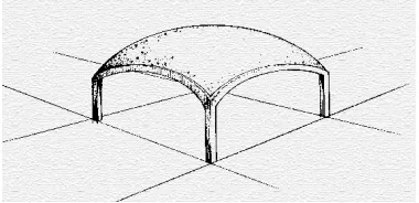
Geodesic dome is one of the simplest forms of structure which has a very unique spherical

or partial-spherical shape. The skeleton of the structure consists a number of unequal and

straight structural members to form its many stable triangular elements in order to provide

resistance to the gravitational, wind and seismic loads. The geodesic dome has the capacity

to achieve large span without any form of internal posts, load bearing walls or deep beams

or trusses, the load is evenly distributed through the surface of the dome. On the other side,

a conventional building would require more material and space to achieve larger span, and

deflection control and bracing requirement may become a challenge for the conventional

form. Whereas, the geodesic is very effective in limiting deflection, and it is self-braced

through its stable triangulated elements.

Geodesic domes can be constructed from various materials, (e.g. timber, steel) and a very

light PVC cover is applied to the outside of the main structure to shield the dome from

weathering. It provides a strength-to-weight ratio that many others could not compete. The

fast speed of erection, competitiveness in material costs and its resilience to natural

disasters have made dome construction applicable to many agricultural, commercial

applications.

The purpose of this report is to present the background information about geodesic dome,

also to verify a designing methodology and to develop design procedure based on the most

critical loading, that is wind load for this type of structure. The aid of computational

analysis has been considered as the key tool to obtain design data from the complex 3D

dome model, and then manually checked against steel structure standards AS 4100-1998.

In addition, an Excel spreadsheet was developed using finite element analysis method to

extract the forces for each element, then the results were compared against the outcomes

from computational analysis method for validation purpose. The spreadsheet was aimed to

standardize the design procedure and to reduce the time required for analysis and design in

the future, and sensitivity analysis could also be conducted easily and quickly using the

ii

Faculty of Health, Engineering and Sciences

ENG4111/ENG4112 Research Project

Limitations of Use

The Council of the University of Southern Queensland, its Faculty of Health, Engineering

& Sciences, and the staff of the University of Southern Queensland, do not accept any

responsibility for the truth, accuracy or completeness of material contained within or

associated with this dissertation.

Persons using all or any part of this material do so at their own risk, and not at the risk of

the Council of the University of Southern Queensland, its Faculty of Health, Engineering

& Sciences or the staff of the University of Southern Queensland.

iii

Certification

I certify that the ideas, designs and experimental work, results, analyses and conclusions

set out in this dissertation are entirely my own effort, except where otherwise indicated and

acknowledged.

I further certify that the work is original and has not been previously submitted for

assessment in any other course or institution, except where specifically stated.

Zhuohao Peng

iv

I would like to express my appreciations to everyone that has been involved in assisting me

prepare and complete this project. The following people and organisations that I would like

to make special mention of for without their support I would not have been able to complete

this project.

•

Dr Sourish Banerjee for instructive supervision, guidance and suggestions, as well

as his valuable time and effort.

•

Bentley

sponsorship of a free license of Microstran V9 over the period of the

project.

•

Strata Group Consulting Engineers for providing the idea of the project and

supporting me completing the project.

•

Family for selfless supports over the years in many ways to encourage and support

me.

v

Table of Contents

Abstract ... i

Certification ... iii

Acknowledgements ... iv

Table of Contents ... v

List of Figures ... viii

List of Tables ... x

Nomenclature ... xi

Novel Aspect ... xiv

1.

Introduction ... 1

1.1

Background Information ... 1

1.2

Project Aim and Objectives ... 2

1.3

Scope and Limitation ... 3

2.

Literature Review ... 4

2.1

Introduction ... 4

2.2 Shell Dome ... 4

2.3

Geodesic dome ... 5

2.3.1

History ... 5

2.3.2

Geometry ... 6

2.3.3

Coordinate System ... 9

2.3.4

Strength and weakness ... 10

2.3.5

Structural analysis of dome ... 10

2.3.6

Failure Modes... 11

2.4

Loading ... 12

2.4.1

Wind Load ... 12

2.4.2

Seismic load ... 13

vi

3.

Model Generation and Loading ... 15

3.1

Geodesic Model Generation ... 15

3.2

Loading ... 16

3.2.1 Wind ... 16

3.2.2

Self-Weight and Imposed Load... 21

3.2.3

Load Combination Cases ... 22

3.3

Assumptions ... 23

4

Excel Spreadsheet Development ... 24

4.1

Introduction ... 24

4.2

Flow Chart and Spreadsheet Structure ... 24

4.3

Data Input ... 25

4.3.1

Nodal Coordinates and Strut Information ... 25

4.3.2

Loading ... 25

4.4

Member Stiffness Matrices Construction ... 27

4.5

Global Stiffness Matrices Construction ... 31

4.6

Solution Procedure ... 33

4.7

Post Procedure ... 34

4.8

Design Procedure ... 35

5

Microstran V9 Analysis ... 38

5.1

Introduction to Microstran V9 ... 38

5.2

Model Setup ... 38

5.3

Load Input ... 39

5.4

Structural Analysis ... 40

6

Conclusion ... 42

6.1

Comparison of Outcomes ... 42

6.2

Future Work and Improvements ... 44

Reference ... 1

vii

Appendices C – Spreadsheet ... 9

viii

Figure 1: Translation shell dome (Ketchum) ... 4

Figure 2: Regular Octahedron (Kenner 2003) ... 6

Figure 3: Modified Octahedron (Kenner 2003) ... 7

Figure 4: Class and frequency (Salsburg) ... 7

Figure 5: 31 great circles (Pacific Domes 1971) ... 8

Figure 6: Icosahedron and great circle (Kenner 2003) ... 8

Figure 7: Six great circles on the spherical icosahedron (Kenner 2003) ... 9

Figure 8: The spherical co-ordinates (Ramaswamy 2002) ... 9

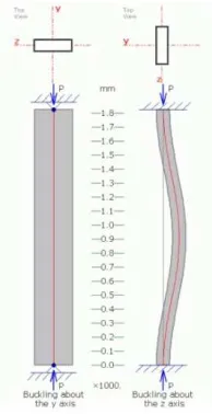
Figure 9: Strut buckling (Lewis 2005) ... 11

Figure 10: Wood dome on shake table (Clark 2014) ... 13

Figure 11: 6m V2 Geodesic dome model generated CADRE Geo 6.0 ... 15

Figure 12: Illustration of wind acting on dome structure (Susila 2009) ... 16

Figure 13: Elevation of circular dome (Susila 2009) ... 17

Figure 14: External Pressure coefficient Cp, e for y/d = 1/2 (Susila 2009) ... 17

Figure 15: External Pressure Coefficient (Cp, e) – Curved Roof (AS/NZS 1170.2 2011) 18

Figure 16: Dome wind zone divisions ... 19

Figure 17: Elevation of dome and tangent line ... 19

Figure 18: Tributary areas of a node ... 22

Figure 19: Flow chart of FEA procedures ... 24

Figure 20: Nodal coordinates and reference diagram ... 25

Figure 21: Wind loads local and global axis ... 26

Figure 22: Loads of primary and combined load cases ... 27

Figure 23: Load – displacement relationship ... 27

Figure 24: Three-dimensional system ... 29

Figure 25: Member stiffness matrix ... 30

Figure 26: Node designation of the geodesic dome ... 31

Figure 27: Strut designation of the geodesic dome ... 32

Figure 28: Structure global stiffness matrix assembling ... 33

Figure 29: Global stiffness matrix and partition ... 33

Figure 30: Calculation of nodal deflection ... 34

Figure 31: Calculation of strut axial force ... 35

Figure 32: Effective length factors for members for idealized conditions of end restraint

(AS4100:1998) ... 36

ix

Figure 36: Imposed load assignment (Q) ... 39

Figure 37: Wind load assignment (Wind) ... 40

Figure 38: Axial force diagram ... 40

Figure 39: Deflection under wind load ... 41

Figure 40: Geodesic dome with two section sizes ... 44

x

Table 1: Relationship between NZS3604 wind zones, site wind speeds and basic pressures

xi

A

Cross section area

A

Gross cross section area

A

Net cross section area

C

Wind pressure coefficient

C

External wind pressure coefficient

C

Internal wind pressure coefficient

C

Aerodynamic shape factors

CHS

Circular Hollow Section

d

depth of geodesic dome

d

Local displacement matrix

d

Local displacement at near end

d

Local displacement at far end

DOF

Degree of freedom

D

Global displacement matrix

DXF

AutoCAD drawing interchange format

D

Global displacement in x axis at near end

D

Global displacement in y axis at near end

D

Global displacement in z axis at near end

D

Global displacement in x axis at far end

D

Global displacement in y axis at far end

D

Global displacement in z axis at far end

D

Nodal deflections matrix

D

Boundary condition of nodes matrix

E

Modulus of Elasticity (MPa)

f

Steel yield strength

f

Steel tensile strength

FEA

Finite element analysis

G

Dead load

h

height of geodesic dome

k’

Member stiffness matrix

k

Internal combination factor

k

External combination factor

k

Area reduction factor

xii

k

Effective length factor

k

Correction factor

kPa

Kilopascal

kg

Kilogram

kN

Kilo newton

K

Structure stiffness matrix

L

Length of strut

N

Nominal section capacity

N

Nominal member capacity

N

Maximum Axial compression force from Excel

N

Maximum Axial compression force from Microstran

N

Nominal tensile capacity

N

Maximum Axial tensile force from Excel

N

Maximum Axial tensile force from Microstran

PVC

Polyvinyl Chloride

q

Axial force

q

Local axial force at near end

q

Local axial force at far end

Q

Live load / Imposed load

Q

Global force in x axis at near end

Q

Global force in y axis at near end

Q

Global force in z axis at near end

Q

Global force in x axis at far end

Q

Global force in y axis at far end

Q

Global force in z axis at far end

Q

Axial forces matrix

Q

Reaction forces matrix

r

rise of geodesic dome

R

Unit length from the centre

R

Principal radii of curvature

T

Displacement transformation matrix

T

Transpose of displacement transformation matrix

T

Thickness of the a shell slab

W

Wind load

xiii

z’

Local z axis

ε

Strain

σ

Stress

φ

Reduction factor

φ

Meridian of longitude

θ

Latitude

λ

/cos

θ

Smallest angle between positive x global axes and x' local axis

λ

/cos

θ

Smallest angle between positive x global axes and y' local axis

λ

/cos

θ

Smallest angle between positive x global axes and z' local axis

∆

Displacement / Deflection (mm)

∆

Vertical displacement of node 1 from Excel

∆

Vertical displacement of node 1 from Microstran

ν

Frequency

α

Member slenderness reduction factor

(U)

Windward quarter

(T)

Centre half

xiv

The initial idea of this project came from a local business in the Hawke’s Bay, New Zealand.

The business owner was seeking a local engineer to carry out a structural design of geodesic

domes with different diameters for the potential dome renting business. The proposed

domes were targeted for temporary event veneer, semi-permanent farming structure, and

post-disaster structures.

The local business has approached Strata Group Consulting Engineers for expression of

interest. At the time, I was seeking feasible and challenging project ideas for the final year

project in order to complete my Bachelor of Engineering degrees. The task was given to

me by the director of Strata Group Consulting Engineers to carry out further research and

study.

Due to the uniqueness of the structure shape and lack of previous dome design experience

internally, the project had to start from scratch requiring extensive research. From the initial

research, loading analysis, model setup, to structural analysis and structural design, all of

the tasks were carried out by my own work. The challenges for dome structure were to

estimate the wind load on the structure, to understand the geometry formation of the

structure, as well as to develop a feasible theoretical approach to fast track the analysis and

1

1.

Introduction

1.1

Background Information

Natural disaster resilient and cost effective structure has been put under spotlight for

decades. The financial and psychological burden of natural disasters have impacted almost

every country in the world where suffered from natural disasters such as earthquake,

hurricane, etc.

Looking over New Zealand natural disaster chronicle, in 3

February 1931, Hawke’s Bay

earthquake, a magnitude of 7.8 strokes, killing 256 lives and devastating the Hawke’s Bay

region. In February 2011, a magnitude of 7.1 hit Christchurch, the second largest city in

New Zealand, claims 185 people’s lives, thousands were affected. The building standard

has been constantly reviewed and lifted to safeguard safety of the publics. Pre-1931, NZ

building code only required 2% of gravity load (0.02G) to be designed for lateral load, but

the latest code could have more than 100% of the gravity load (1.0G) laterally applied to

the structures, depending on the earthquake zone, soil type and other facts. The increasing

requirements from the fast changing design codes has being constantly challenging all the

building professionals in the ways of strength, functionality, architecture and costing

worldwide.

The increasing demands of lighter, stronger and cheaper materials have prompted many

architects, scientists, engineers to seek new technology and building concepts to achieve

the goals. Taking earthquake for example, the lighter the structure it is the lesser lateral

force will be recruited during an earthquake event. And with stronger and lighter material,

the designers are able to achieved more span, space and functions.

In the late of 1940s, Buckminster Fuller a well-known American architect, mathematician

and engineer began to experiment with the geodesic geometry. He noticed that natural

structures seemed to have better performance against naturally occurring disasters whereas

the conventional building forms, e.g. rectangular shaped building would inherently have

some issues from its geometry. The difference between a dome structure and a rectangular

structure can be simply described as the strength variation between a triangle and a

rectangle withstanding external pressure or load. The rectangle would deform sideway

2

change accordingly. The simple triangle shape would however retain its shape and inner

angles, due to the triangle shape being self-braced and stabilized. On the other side, a

rectangle would require some forms of bracing elements or rigid connections in its

geometry to lock itself in place. This principle has inspired Fuller with his study of creating

new architectural design, the geodesic dome consisting of a series of triangles to achieve

exceptional strength to weight ratio.

On the other side, light-weighted structure has its own challenge. For instance, in the event

of typhoon and cyclone, the mass of the building itself that is considered very efficient

against pressure generated by the flow of air, which has a tendency to topple or uplift the

building. Specifically, in Australia and the regions that cyclone is treated as a frequent

natural disaster, as well as in the rural or less populated areas where shielding or obstacles

from the buildings in the vicinity is difficult to achieve. This situation applies to many

farming and agricultural structure, high rise buildings, and the areas near the coast.

1.2

Project Aim and Objectives

The form of dome has never been widely adopted as a popular structural form in the

building construction due to its complex shape and difficulty for modelling and analysis

comparing to conventional structures. As an outstanding conceptual and architectural form,

dome shaped structure remain underutilized despite of its high potential and exceptional

performance in many ways.

This project examines a prototype of a 6m diameter, 3m high geodesic dome in a high wind

zone with a maximum wind speed of 50m/s (180km/h), this equivalent to 1.50kPa in terms

of pressure (kPa). The reason for choosing a smaller and simpler dome configuration was

to consider the complexity of mathematical model, and time restraint of the project from

the University of Southern Queensland.

A spreadsheet was proposed for the dome described above to fast track the analysis and

design procedures, so that sensitivity analysis was able to be conducted efficiently and

accurately. A computer based program was used for comparison and validation of the

spreadsheet proposed.

3

•

Research various types of geodesic domes to establish a suitable model for the size

of the proposed dome.

•

Study how wind reacts around spherical shaped structures, find out adequate

methods that can be used for this project.

•

Choose and calculate the primary load cases and load combination cases that are

appropriate and adequate for the project using standard AS/NZS 1170.0.

•

Develop calculation template using FEA method in the environment of Excel

spreadsheet.

•

Comparing FEA method outcome with the commercial computer package

Microstran V9

outcome in order to validate the spreadsheet developed.

•

Carry out structural design from the results obtained from FEA and Microstran V9

using AS4100-1998.

•

Conclude and comment on the outcome of the project based on the finding.

•

Identify future works and recommendations

1.3

Scope and Limitation

A 6m diameter, frequency 2V geodesic dome was proposed for this research project due to

the time restraint of the project and geometric complexity of higher frequency for larger

domes. Hence, a relatively smaller and simpler dome has been adopted in order to achieve

the objectives and aims. However, spreadsheets will be developed for larger and more

complex geodesic domes in the future.

Connection and foundation design were not proposed for this dissertation due to the time

frame and resources. The primary loadings that were considered for the project were dead

load, live load and wind load. The earthquake load was not included as the light weight

structure does not attract a lot of forces during the seismic event. Hence the seismic load

was not considered to be the governing load for the design. Other loading such as snow

load was also not considered in order to simplify the load calculations. However, the snow

load can be easily included if it is required in the future design.

4

2.

Literature Review

2.1

Introduction

The purpose of this literature review is to establish a framework to the relevance of the

work undertaken in this dissertation, and to define terminology and definition to assist

understanding of the report, as well as to identify the research, study area required to

support the dissertation.

2.2 Shell Dome

Scrivener said that the shell dome has a thin curved slab whose thickness t is small

compared with the other dimensions and in particular compared with the principal radii of

curvature R

of the surface. In the most practical applications, where the ratio of t/R

is

between 1/1000 and 1/50 is considered to be thin shell dome. However, an upper limit of

the thickness t/R

< 1/20 was recommended. When the ratio of t/R

becomes relatively large,

and the shell may be classified as thick, the problem of analysis changes from a two

dimensional to a three dimensional problem with a very great increase in length and

complexity of analysis. The membrane theory can be used for analysis of the shells, where

membrane theory assumes that there are no moments in the shell, hence load resistance is

by means of direct tensions or compressions and in-plane shears only. Alternatively, the

analysis of shells can be conducted by the use of the finite element method, where the shell

surface is divided into a number of discrete elements each of which must satisfy the

equilibrium and compatibility requirements.

5

Shell dome is one of the sub-family of the dome structure, it inherits and shares the most

of advantages and geometric properties of the dome structure. A shell dome requires very

different approach for analysis and design, therefore, the shell dome was not included the

scope of this research dissertation.

2.3

Geodesic dome

2.3.1 History

The earliest geodesic dome construction was as early as 1919 the Berlin based Walther

Wilhelm Johannes Bausersfeld (*1879, †1959

started the development of a dome structure

for the purpose of projections in Jena, Germany (Makowski 1979).

In the late 1940’s, R. Buckminster Fuller (*1895, †1983

developed and named the

geodesic dome from field experiment with Kenneth Snelson and others at Black Mountain

College (Giulio 2006). Because the efforts of Buckminster Fuller, the term of “geodesic”

was known to the others.

In 1953, Fuller designed a dome to cover the 28m diameter Ford Motor Company’s

headquarters building. The dome consisted of 12,000 aluminium struts weighing a total of

1,700 kg that were preinstalled and then lifted into position (Encyclopedia.com).

The following year, Fuller received a patent on the geodesic dome system. Fuller has

predicted that a million geodesic domes would be erected by the mid of 1980s, but by the

early 1990s, the estimated worldwide number was somewhere between 50,000 and 300,000

(Encyclopedia.com). Newsday (1992) reported that the majority of geodesic dome

structures have been built for green-houses, storage shed, defence shelters, and tourist

attractions.

In 1982, the 48m diameter sphere at Walt Disney World’s Epcot Centre, named Spaceship

Earth, which was coined by Fuller, who also developed the structural mathematics of the

6

2.3.2 Geometry

2.3.2.1 Geodesic Subdivision

Buckminster Fuller’s geodesic model was based on the sphere subdivision of an

icosahedron although geodesic domes have been designed using octahedron and

dodecahedron to evade Buckminster’s patent. For the reason of clarity of presentation, a

simpler octahedron is used to demonstrate the concept of subdivision, class and frequency

ν

.

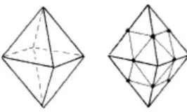
Figure 2: Regular Octahedron (Kenner 2003)

The left shape in Figure 2 shows a regular octahedron, having eight equilaterally triangular

faces. The right shape in Figure 2 shows each face of the octahedron divided into four

smaller triangles by simply connecting the midpoints of each edge. The 32 small triangles

are equilateral too, but the octahedron does not look alike a sphere. This is because the

distance from the centre of the octahedron to the vertices and to the midpoint is different.

From Figure 3, the midpoints at each edge are pushed away from the centroid until they

have the same length as other vertices from the centre. It is clear that the

∆

m

, m

, m

is

equilateral as all the vertex points were moved the same distance.

∆

A, m

, m

,

∆

B, m

, m

,

and

∆

C, m

, m

are not equilateral but isosceles. Hence, there are a total number of 4

equilaterals, and 24 isosceles in the modified octahedron as shown in Figure 3. This process

7

Figure 3: Modified Octahedron (Kenner 2003)

The concept of frequency is defined as the number of parts or segments into which a

principle side is subdivided. For instance, 2

ν

means the edge of the principle triangle is

equally divide into 2 segments, 3

ν

means 3 equal segments and so on. There are two classes

of geodesic subdivision as shown in Figure 4, for Class

Ι

, and dividing lines are parallel to

the edges of the principle triangle, whereas, Class

ΙΙ

, having the dividing lines

perpendicular to the edges of the principle triangle.

Ramaswamy (2002) summarise that Class

Ι

subdivision permits both odd and even

frequencies, but Class

ΙΙ

subdivision can only be achieved with an even frequency of

subdivision. And Class

ΙΙ

subdivision results in a smaller inventory of different lengths, but

a larger variation between lengths, hence the stress distribution is less uniform in Class

ΙΙ

subdivision. Class

Ι

subdivision has uninterrupted equator at all even frequencies.

Additionally, Class

ΙΙ

domes can only be achieved with an even frequency of subdivision.

Odd order frequency domes cannot produce a hemispherical shape as an equatorial

perimeter ring is only produced for even order frequencies.

8

2.3.2.2

Geodesic Great Circle

Kenner (2003) says that geodesics is a technique for making shell-like structures that hold

themselves up without supporting columns, by exploiting a three-way grid of tensile forces.

The geodesic dome is sliced from one of the complex polyhedral, it has a large number of

triangular faces, all approximately, but not quite equilateral. The struts that bound them

follow the paths of great circles, sometimes complete, more often interrupted.

Pacific Domes (1971) explains that a plane that passes through the centre of a sphere is

called a great circle plane. A great circle cuts a sphere exactly in half. Fuller has discovered

that there are 31 great circle planes produced by different rotations of the icosahedron, as

shown in Figure 5.

Figure 5: 31 great circles (Pacific Domes 1971)

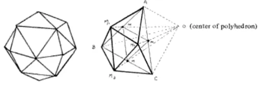
Figure 6 shows an icosahedron, note the five triangles meeting at each vertex. This

five-way vertices are called pents (after the pentagons that surround them). From each pent

centre radiate portions of five great circles. Each has its centre at the centre of the system.

Each sets off on a 360

circuit, of which it completes about 63.5

before bumping into

another pent centre (Kenner 2003).

9

The icosahedron can be projected onto a sphere to form a spherical icosahedron as shown

in Figure 7.

Figure 7: Six great circles on the spherical icosahedron (Kenner 2003)

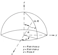
2.3.3 Coordinate System

Mathematically, there are two systems of generating geometric coordinates: Cartesian and

polar. Kenner (2003) specify that the polar coordinate system is also called the

spherical-coordinate system, which consists two angles

φ

and

θ

, together with a distance or radius r

to specify a unique point. The first angle

φ

coordinate resembles a meridian of longitude,

whereas the second angle

θ

coordinate resembles a specification of latitude, and R

coordinate measures the unit length from the centre.

Figure 8: The spherical co-ordinates (Ramaswamy 2002)

The polar coordinate system is particularly suitable for generating spherical geometries.

However, in the context of computer aided structural analysis programmes, Cartesian

coordinate system was adopted for developing software packages. Hence, the coordinates

10

2.3.4 Strength and weakness

Geodesic dome has very low centre of gravity than any other cubic or square structures of

similar proportions. The light weight and rigid triangulated skeleton skin is able to enclose

a large area without the need for internal supports, e.g. load bearing walls, posts etc. The

shape of the structure is capable of evenly distributing the stress through the structure, this

property performs extremely well under seismic event. Due to the even stress distribution

and light weight of the construction material, the foundation is most likely to be the simpler

and much cheaper shallow foundation.

On the other side, the complex geometry shape demanding of more advanced mathematics

for structural analysis and computer modelling. The aesthetic appeal of the dome is not

always appreciated by everybody; this is very subjective to the individual. The most

common complaints are regarding the partitioning of large space to achieve functions, and

loss of space due to the curved roof and wall.

2.3.5 Structural analysis of dome

Ranzi (2015) says that the stiffness method is a powerful approach for the analysis of

statically determinate and indeterminate structure and its popularity is mainly attributed to

its ability to be easily programmed for computer calculations due to its well defined

solution procedure. For stiffness structural analysis, the model need to be break down into

sets of simple, idealized elements connected with nodes. The basis of the stiffness method

for a structure limited to pin jointed elements is that every member acts as a spring, so when

an axial force F is applied which causing the element to deform a distance of

∆

. Kardysz.

et al. (2002) mentioned that a dome which is not fully triangulated is not kinematically

stable when idealised as a truss and stiffness may vary greatly in different directions on

dome’s surface. Hence, only the method for a space truss system will be discussed in the

11

2.3.6 Failure Modes

Lewis (2005) reports that the most likely cause of structural failure has to be examined.

The weakest member in the structure is determined by comparing the magnitude of force

for each failure mode.

Failure mode 1: Strut Buckling

The buckling strength of the longest member in the system needs to assessed in accordance

with AS4100-1998. A member is likely to become unstable before reaching its yielding

capacity when under axial compression, and the buckling capacity of a member would be

greatly reduced if there was a bending moment along the member as well as the

compressive stress, then the combined strength of flexural and compression will need to be

checked. However, the idealised model of FEA assume that the pins at each end are

frictionless, and the member will only undergo internal axial forces. Therefore, only the

compression and tensile capacity of the member were calculated against the demand.

Figure 9: Strut buckling (Lewis 2005)

Failure mode 2: Tie Yielding

The yield strength of the member in the system needs to be assessed in accordance with

AS4100-1998. This failure mode is unlikely to occur comparing to other failure modes.

12

compressive forces should be reasonably close due to the unique property of geodesic dome

that stress was evenly dissipated through the structure. As explained above, the member is

likely to buckle before reaching its yielding capacity, for this reason, buckling failure under

compression stress is more critical than the tensile yielding failure.

Failure mode 3: Connection Bolt Shear Failure

Strut fasteners are M12, grade 8.8 bolts at each intersection of the structure. The maximum

axial force will be used to determine the shear capacity required for the bolt. Also the shear

failure of the strut material directly connecting may occur before the bolt failure. Lewis

(2005) concludes that the localise yielding in this region is not likely to result in a

catastrophic failure of the entire structure but an elongation of the bolt hole. However, this

would be problematic if the structure is under repetitive load over a long period of time.

The design check for this failure mode was not included in this research.

2.4

Loading

2.4.1 Wind Load

The site wind speed was determined based on the Australia & New Zealand wind load

standard AS/NZS 1170.2:2011. The code provides guidance for calculating the wind

pressure coefficient on curved structures.

ASCE 7-98 recommends three different approaches for estimating wind pressure which are

simplified procedure, analytical procedure and wind tunnel procedure. In the analytical

procedure, the wind coefficient is obtained from AS/NZS 1170 by computing the combined

effect of internal and external pressure. For simplicity, wind forces were considered to act

on one large area of the structure rather than individual members. However, Cheng. Et al.

(2008) reported that the curved shape of dome makes the accurate estimation of the wind

pressure fluctuations on a hemispherical dome a difficult task due the Reynolds number

effects. There have been record of collapse of curve shaped storage domes due to inaccurate

and inadequate estimation of wind pressure. Hence, an experimental method is needed to

be carried out for determining information on local wind patterns, wind pressure coefficient,

and wind-induced structural vibration. Wind tunnel test has been widely used to investigate

13

test, a scaled model is made to the exact shape of the objective structure, and then the model

is placed in the wind tunnel for the test, and experimental data are recorded for analysis.

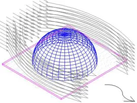
Besides all the procedures mentioned above, interestingly, Susila (2009) recommend that

using CFD (Computational Fluid Dynamic) to replace the wind tunnel testing to predict

pressure coefficient and other parameters intended. CFD treats air flow as fluid flow, it

uses numerical methods to simulate air turbulent around a structure, and then the pressure

and suction distributions on the surface of the model are obtained. However, this method

requires very complex mathematic calculation and computer simulation, which is out of

scope of this report. For the purpose of the research report, the conservative outcome was

adopted from the comparison of wind tunnel test and code requirement in order to insuring

the results are not underestimated.

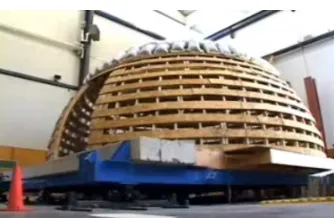
2.4.2 Seismic load

The self-weight of the dome is relatively light, hence the seismic analysis could be

neglected from this research, unless there is a requirement for the dome to support a heavy

object. Clark (2014) has reported that in April 2005, at the University of British Columbia

in the Department of Civil Engineering’s Earthquake Engineering Research Facility, a

7.3m diameter wooden framed dome was put into seismic test on a shake table

. The dome

survived without damage under simulations of several real earthquake events and even

heavily load

(10 tons of sand bags as well as 8.5 tons of steel plates, which is an additional

of 24 tons in total). The weight of the geodesic dome proposed in this research project is

very light, the seismic load on the structure was not considered to be critical, and hence

neglected from loading calculations.

Figure 10: Wood dome on shake table (Clark 2014)

2

This is a device for shaking structural models or building components with a wide range of

simulated ground motions, including reproductions of recorded earthquakes time-histories.

14

2.4.3 Self weight and imposed loads

The self-weight of the proposed geodesic dome includes the weight of the member (steel

hollow sections), connection and cladding. The cladding proposed was a very light

waterproof PVC coating with a maximum unit weight of 0.01kPa. A 0.25kPa imposed load

was also considered as the loading from construction workers and equipment during

construction and maintenance.

2.4.4 Snow load

Snow load was not considered in this research. However, the snow load must be considered

in some areas where heavy snow is likely to occur. The proposed geodesic dome was not

designed to take snow load; hence the cladding of the structure must be taken off to avoid

catastrophic structural failure when there is an event of snow. The snow load will be

15

3.

Model Generation and Loading

3.1

Geodesic Model Generation

The Polar and Cartesian coordinate system systems have been introduced in section 2.3.3.

The Cartesian coordinate system was adopted for developing mathematical model as the

local and global stiffness matrices can be easily expressed by Cartesian coordinates without

further complicated conversion.

Hence, a commercial package called CADRE Geo 6

was used to generate vertices and

struts and ties for the proposed geodesic dome. CADRE Geo is a design utility software

that can generate a wide variety of 3D geodesic and spherical or ellipsoidal models for

import to CAD or other structural analysis applications. The data generated by CADRE

Geo 6 can be represented in the form of tables containing detailed information of hubs,

struts and panels. The tables were then saved into Excel spreadsheet for future reference

and utilisation of stiffness method.

Figure 11: 6m V2 Geodesic dome model generated CADRE Geo 6.0

The 6m diameter, Class I, frequency 2V geodesic dome includes a total of 26 nodes, and

65 line elements or members. There are four types of hubs depending on the angle to the

neighbour hub and number of members connecting to the hub. The members have two

different lengths A and B, type A has a length of 1.6396 meter and type B is slightly longer

with a length of 1.8541 meter. There are a total of 10 nodes are at ground level out of 26

16

nodes, these nodes were considered as the boundary conditions as they are anchored to the

ground to provide lateral restraint to the movement in all x, y and z axis.

3.2

Loading

This chapter introduces all the possible loads that should be considered for the geodesic

dome structure design. These loads including: dead load (G), live load (Q), wind (W).

Seismic load and other loads were excluded from this research report.

3.2.1 Wind

The Australia & New Zealand wind load standard AS/NZS 1170.2: 2011 was used to seek

guidance for calculating the wind pressure coefficients on dome structures.

The curved shape of dome makes the accurate estimation of the wind pressure fluctuations

on a hemispherical dome a difficult task due the Reynolds number effects. There have been

record of collapse of curve shaped storage domes due to inaccurate and inadequate

estimation of wind pressure (Cheng 2008). Hence, an experimental method can be carried

out for determining information on local wind patterns, wind pressure coefficient, and

wind-induced structural vibration. Wind tunnel test has been widely used to investigate and

obtain information regarding wind-induced issues. At the beginning of the wind tunnel test,

a scaled model is made to the exact shape of the objective structure, and then the model is

placed in the wind tunnel for the test, and experimental data are recorded for analysis.

17

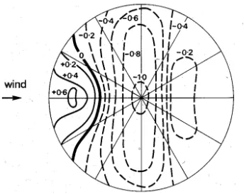
Figure 13: Elevation of circular dome (Susila 2009)

The wind tunnel tests result is greatly depending on the geometry of the dome structure,

and it is very difficult to obtain a reliable relationship between the real dome structure and

wind tunnel tests. The geometry of the dome is defined as height over depth y/d, where y

measures the height of the dome above the ground, and d is the depth or diameter of the

circular dome. The ratio of y over d plays a very important role in wind tunnel test outcomes,

the pressure coefficient value C

increases as the y/d ratio increases. From Figure 14, where

the ratio of y/d = 0.5, the following observations can be made:

i.

The maximum positive pressure C

(+0.6) occurs at 0

.

ii.

The maximum negative pressure C

(-1.0) occurs at top of the dome.

iii.

A greater portion of the dome is affected by suction.

Figure 14: External Pressure coefficient Cp, e for y/d = 1/2 (Susila 2009)

Notice that the negative coefficient meaning that the wind is acting away from the surface

of the dome which has a suction effect. On the contrary, the positive coefficient indicates

18

Alternatively, from AS/NZS 1170.2:2011, the external pressure coefficients (C

) of

domed roofs with profiles approximating a circular arc, wind directions normal to the axis

of the roof shall be obtained from Figure 15.

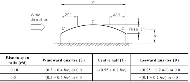
Figure 15: External Pressure Coefficient (Cp, e) – Curved Roof (AS/NZS 1170.2 2011)

The dome is rising directly from the ground, hence h = r, h/r = 1, and r/d = 0.5. From Figure

15, the external wind pressure coefficients can be calculated as the following:

i.

at windward quarter (U) equals (0.5 - 0.4 x 1.0) = +0.1

ii.

at the centre half (T) equals – (0.55 + 0.2 x 1.0) = -0.75

iii.

at leeward quarter (D) equals – (0.1 + 0.2 x 1.0) = -0.3

In comparison, both wind tunnel test and wind code have derived similar wind coefficient

around the dome, that is the windward quarter always has positive wind pressure, whereas

the negative wind pressure reaches its maximum value at the centre half and decrease

markedly towards the leeward quarter. Despite that the wind tunnel method offers very

precise patch loading contours, however it is extremely difficult to apply this wind load on

the tributary areas due to the complex load pattern and variability. Hence, as stated above,

according to AS/NZS 1170.2:2011 the dome is divided into three zones such as windward

quarter (U), centre half (T) and leeward quarter (D), as shown in Figure 16. Therefore, the

nodal forces can be computed separately based on the median external wind pressure

coefficient in each zone and its corresponding tributary area.

From Figure 14, the median external wind pressure coefficients have been selected as

19

i.

for windward quarter (U), C

of +0.3

ii.

for centre half (T), C

of -0.6

iii.

for windward quarter (U), C

of -0.4

Figure 16: Dome wind zone divisions

By comparing two set of external wind pressure coefficients, the conservative outcome set

was adopted for the further loading calculation, where (U) C

is +0.1, (T) C

is -0.75 and

(D) C

equals -0.3.

Figure 17: Elevation of dome and tangent line

The tangent line for each node on the dome is different, in order to simplify the loading

calculation, the average tangent angle of 45

was assumed to all the nodes. Hence, the

lateral wind load on a node is sin45

F

node

, and similarly, the vertical wind load is computed

20

From 1170.2:2011, the basic wind pressure and onsite wind speed can be calculated based

on the location, and its corresponding terrain categories, shielding multiplier, topographic

multiplier etc. The purpose of this project is to design the geodesic dome for the targeted

wind zone or wind pressure, so that the structural elements size can be determined to meet

the code guidelines and requirements for the provision of safe and efficient design. The

table 1 shows the relationship between NZS3604 wind zones, site wind speeds and basic

pressure.

Zone

Site wind speed

Basis

Pressure

Metservice

Description

Beaufort

Scale

(m/s)

(km/h)

(kPa)

Low

32

115

0.61 C

Strong gale

9

Medium

37

133

0.82 C

Storm

10

High

44

158

1.16 C

Violent storm

11

Very High

50

180

1.50 C

Category

1

hurricane

12

Table 1: Relationship between NZS3604 wind zones, site wind speeds and basic

pressures. (Shelton 2009)

A very high wind zone was adopted to accommodate for the most of areas and applications.

Hence the basic design pressure is 1.5

C

(kPa), where C

is the aerodynamic shape factors that

were to be determined as shown blow:

, = ,

,

(1)

, = ,

,

(2)

Conservatively assuming that K

, K

, K

and K

is 1.0, and combining equation (1), (2)

we have

= , − ,

(3)

Assuming that the PVC coating of the dome are equally permeable, reading from AS/NZS

1170.2 Table 5.1(A), the internal pressure coefficient C

is equal to -0.3 or 0.0 whichever

is the more severe for combined forces. In this case, the worse internal pressure coefficient

for combined effect is 0, as when C

is equal to -0.3, the negative internal pressure cancels

out some of the negative suction wind acting away on the external surface. Hence the

combined internal and external wind coefficient C

remains unchanged due to C

being

21

3.2.2 Self-Weight and Imposed Load

The main components of self-weight consisting the weight of steel members and the PVC

coating. The light weight waterproof PVC coating only weighs approximately 1000g/m

,

which equals to 0.01 kPa. Assuming that the steel struts used for the 6m geodesic dome is

33.7x3.2 CHS, the mass per linear meter is 2.4 kg/m, which equivalents to 0.024 kN/m.

The self-weights were initially represented using area load function and gravity function

from Microstran V9. These nodal forces are automatically calculated at each node when an

analysis was run. However, in order to ensure that the auto generated forces are directly

comparable to Excel, these auto functions were discarded in favour of the spreadsheet

calculation. Hence, each nodal forces were manually entered at each node in Microstran

V9 based on the concept of tributary area subdivision as shown in Figure 18.

From Figure 18, each node is surrounded by either 5 or 6 triangles, and each triangle has

two possible combinations of the two unique strut lengths A and B, either BBB or AAB.

Geometrically, each triangle can be divided into three equal sub triangles by applying angle

bisectors to the triangle. Hence, the tributary area of a node can be calculated by adding the

sub triangles together. To simplify the distributing area procedure, each triangle is assumed

to be equilateral with an edge length of B, which is the longer strut length. The area of an

equilateral triangle is

B

, the area of each sub triangle is

B

.

Hence, the tributary area

of the node bordered by 5 triangles is

B

, whereas, the tributary area of the node with 6

surrounding triangles equals

B

. There is a total of 6 nodes that only border with 5

triangles, and apart from the boundary nodes at the ground level, the rest of 10 nodes have

6 surrounding triangles instead. For the simplicity, a uniform tributary area of

B

has

adopted for all the nodes, where B equal to 1.8541 meter. Similarly, the total length of strut

that is supported by per node can approximated by assuming that the weight of a strut is

shared by two nodes, and for the most of cases, there are 6 struts connecting to a node,

22

Figure 18: Tributary areas of a node

An imposed load of 0.25kPa was applied vertically on the dome to allow equipment loading

and human body weight while installation and maintenance.

3.2.3 Load Combination Cases

The load combination cases were based on section 4 AS/NZS 1170.0 to determine the worst

effect of combined loadings that are likely to occur to the structure over its designed life

span.

1.)

1.2G + 1.5Q

This combination was chosen to determine the most significant gravitational loading

including imposed load. The self-weight was factored as permanent loads, as well as

the live load was factored to allow for temporary loads.

2.)

1.35G

This combination was chosen to determine the most significant loading from factored

self-weigh only. This is to allow more tolerance for approximating

3.)

1.2G + Wind

The downwards wind combined with factored self-weight to determine the worst

downwards loading effect from wind.

23

This combination represents the reduced dead load with suction wind to determine the

worst loading effect for uplift.

3.3

Assumptions

In order to determine the loading on the structure, the following assumptions were made

based on conservative and reasonable considerations.

•

The connections of the structure were assumed to be frictionless and will not

carry any moment. The structure was treated as 3D space truss.

•

The boundary conditions assume that the all the ground level nodes were fully

fixed.

24

4

Excel Spreadsheet Development

4.1

Introduction

This chapter introduces the basic fundamental theory involved to understand the stiffness

method for analysing 3D dome structures using Excel spreadsheet. The simplest element

of the stiffness elements was introduced. This element is assumed to be able to resist only

axial forces and displaces by a small distance in the direction of the axial forces. This

method will then be expanded to include space-truss analysis. However, this method will

involve tedious calculation to do by hand. Hence, Excel spreadsheet will be used to replace

the time consuming tasks. The reader was assumed to have a basic understanding of matrix

mathematics including addition, multiplication, inversion and transposition

. A former

exposure to the stiffness method will be helpful, but is not essential.

4.2

Flow Chart and Spreadsheet Structure

The spreadsheet was divided into multiple sheets, and each sheet was to distinctively define

one or more procedures in the flow chart as show in Figure 19. Firstly, geometry

information and loading were manually written into sheets “Data Input” and “Loading”

respectively. Then member stiffness matrix k, global stiffness matrix K and force vector

Q

were obtained accordingly. Subsequently each loading combination sheet reads the

corresponding data from K and Q

in order to solve the unknown displacement D

and

reaction force Q

. Then the post procedure uses D

to solve for member axial forces in the

structure. The most critical forces were produced for each load combination case and

summarized in the final design sheet for the final design process.

Figure 19: Flow chart of FEA procedures

25

4.3

Data Input

The data input includes coordinates of nodes, strut lengths, loads and material properties.

All the data and information will be used later by Excel spreadsheet to generate matrices,

analysis and design. It is crucial to ensure the quality and integrity of the input data has

been achieved.

4.3.1 Nodal Coordinates and Strut Information

The CADRE Geo 6 generated geometry were manually entered into spreadsheet in tabular

format as shown in Figure 20. A dome model with numbering reference was also attached

for future quality assurance and visual reference.

Figure 20: Nodal coordinates and reference diagram

4.3.2 Loading

The gravitational nodal forces from self-weight of the dome and imposed live loads were

26

sign means that the direction of the forces is pointing down, which is opposite the z axis.

All of the dead loads and imposed loads are negative.

Figure 21: Wind loads local and global axis

The wind loads on each node was computed from the base wind pressure and the combined

wind coefficient at each node as previously discussed in section 3.2.2. The nodal force at

each node was breaking down into two component forces: horizontal x axis force and

vertical z axis force. The positive wind force indicates that the force is acting towards the

surface of the dome, whereas the negative wind force is acting away from the surface. It is

important to note that the wind force cannot be simply add or subtract from each other as

the positive and negative designation of wind pressure only applies in the nodal local axis.

Hence, the loads need to be transferred into global axis of the whole structure. In Figure 21

the positive wind force F1 in the quarter U has a positive horizontal x axis force pointing

in the positive global x axis, and the negative wind force F2 in the quarter D has a negative

horizontal component force also pointing in the positive global x axis. The two horizontal

forces were expected to be added, however, the opposite sign of each force would produce

a subtraction in result. Therefore, in the loading spreadsheet, all the cells that required

conversion has been highlighted for easy reference.

Once all the nodal forces were calculated for the primary loading cases G, Q and Wind,

then the primary loading were factored and recombined to form the proposed load

27

Figure 22: Loads of primary and combined load cases

4.4

Member Stiffness Matrices Construction

In order to construct member stiffness matrix, the dome structure has been broken down

into individual members and nodes. Each member between two pinned nodes was treated

as a spring, so that when an axial force q is applied to the end of a member, the member

carries an internal load causing a length change of

∆

along the member. The relationship

between the applied load q and the corresponding displacement

∆

is also known as the

spring constant or stiffness k' as shown in equation (12).

This section establishes the stiffness matrix for a single dome member using local x', y'

coordinates, as shown in Figure 23. The strut element can only be displaced in its local axis

x’ when the loads are applied along this axis.

28

The stress within the strut elements under the applied loads as shown in Figure 23 can be

expressed as

=

(4)

And from Young’s Modulus definition the axial stress

σ

can be expressed as

=

(5)

Where the strain

ε

equals to ratio of deformation d

over the length L

=

(6)

Substitute equation (5), (6) into equation (4) and rearrange

=

(7)

Hence, in the left axis coordinate of Figure 23, where a positive displacement d

is imposed

on the near end of the strut while the far end is held pinned, the forces developed at the

ends of the strut are

=

= −

Likewise, in the right axis coordinate of Figure 23, where a negative displacement d

is

applied on the far end of the strut while the near end is held pinned, the forces developed

at the end of the strut are

= −

=

Then the resultant forces caused by both displacements can be added as

=

−

(8)

29

The equation (8), (9) can be then written in the form of matrix

=

1 −1

−1 1

(10)

Alternatively, equation (10) can be written as

= ′

(11)

Where

=

−1 1

1 −1

(12)

The matrix k', is called the member stiffness matrix. The first column of the matrix k',

represents the forces in the member when the far end is held as pinned and the near end has

undergone a unit displacement. Multiplying force and displacement transformation

matrices T

, and T to transform the local stiffness matrix k' to a global stiffness matrix k

for each member

.

=

−

−

−

−

−

−

−

−

(13)

Similarly, to include the additional two degrees of freedom in the 3D coordinate system.

Hence, a total of six degrees of freedom for each element, as each node can move in three

global dimensions: x, y and z as shown in Figure 24.

Figure 24: Three-dimensional system

30

In Figure 24, the direction cosines

θ

,

θ

and

θ

between the global and local axis can be

calculated from the coordinates of two nodes. The

θ

,

θ

and

θ

are usually written as

λ

,

λ

and

λ

. Carrying out matrix multiplication once more yields the symmetric matrix k of

N

N

N

F

F

F

=









































−

−

−

−

−

−

−

−

−

−

−

−

−

−

−

−

−

−

λ

λ

λ

λ

λ

λ

λ

λ

λ

λ

λ

λ

λ

λ

λ

λ

λ

λ

λ

λ

λ

λ

λ

λ

λ

λ

λ

λ

λ

λ

λ

λ

λ

λ

λ

λ

λ

λ

λ

λ

λ

λ

λ

λ

λ

λ

λ

λ

λ

λ

λ

λ

λ

λ

λ

λ

λ

λ

λ

λ

F

F

F

N

N

N

(14)

This single member stiffness matrix can be assembled to form the structure stiffness matrix

when the global coordinates for each node are known and correct numbering are assigned

to represent the degrees of freedom of each node. The assembling procedure will be

discussed in the next section.

Firstly, the spreadsheet reads the coordinates from the input table to calculated the smallest

angles between the positive axis, which is

λ

,

λ

,

λ

, and the length of the strut L. Following

equation (14) derived above, each member stiffness matrix was constructed as shown in

Figure 25 below.

Figure 25: Member stiffness matrix

The numbers on the top and on each side of the 6 x 6 matrix are the associated DOF

numbers as shown in equation (14). This DOF number was used as a mapping tool to form

31

4.5

Global Stiffness Matrices Construction

The structure stiffness matrix relates to nodal displacements D and forces vector Q in the

directions of the global axis x, y and z. The total number of global DOFs of the space truss

N

equals to 3 × the total number of nodes N

in the space truss. Hence the structure

matrix K is a N

× N

stiffness matrix, which represented as

=

(15)

The assembling process involves combining the stiffness matrix of each element k

(n

represents the total number of nodes in the structure) into the global structure matrix K.

This procedure was carried out carefully by assigning the DOF numbers of each element

to the global freedoms, each 6 × 6 element stiffness matrix k was to be placed in its same

row and column designation in the structure stiffness matrix K. As shown in Figure 26,

each node in the geodesic dome has been designated with a node number together with

numbers to identify the global DOF at each node, with a natural number of 3n-2 to represent

the global DOF in the x axis, 3n-1 as the global DOF in the y axis and 3n as the global DOF

in the z axis (n = 1,2,3, ……. N

). The first node (node 1) has 1,2,3 assigned to it, whereas

the last node (node 26) has (76,77,78) allocated to its DOF designation. It is a good practice

to code number the unconstrained DOF using the lowest numbers, followed by the highest

numbers assigned to the restrained DOF, this allows simple partition of the structure

stiffness matrix.