A generalised finite difference scheme based on compact
integrated radial basis function for flow in
heterogeneous soils
D. Ngo-Conga,∗, C.M.T. Tiena, T. Nguyen-Kya, D.-A. An-Voa,
N. Mai-Duya,b, D.V. Strunina,c, T. Tran-Conga,b
a
Computational Engineering and Science Research Centre, University of Southern Queensland, Toowoomba, QLD 4350, Australia.
b
School of Mechanical and Electrical Engineering, Faculty of Health, Engineering and Sciences, University of Southern Queensland, Toowoomba, QLD 4350, Australia. c
School of Agricultural, Computational and Environmental Sciences, Faculty of Health, Engineering and Sciences, University of Southern Queensland, Toowoomba, QLD 4350,
Australia.
Abstract
In the present paper, we develop a generalised finite difference approach based on compact integrated radial basis function (CIRBF) stencils for solv-ing highly nonlinear Richards equation governsolv-ing fluid movement in hetero-geneous soils. The proposed CIRBF scheme enjoys a high level of accuracy and a fast convergence rate with grid refinement owing to the combination of the integrated RBF approximation and compact approximation where the spatial derivatives are discretised in terms of the information of neigh-bouring nodes in a stencil. The CIRBF method is first verified through the solution of ordinary differential equations, 2–D Poisson equations and a Taylor-Green vortex. Numerical comparisons show that the CIRBF method outperforms some other methods in the literature. The CIRBF method in conjunction with a rational function transformation method and an adaptive time-stepping scheme is then applied to simulate 1–D and 2–D soil infiltra-tions effectively. The proposed soluinfiltra-tions are more accurate and converge faster than those of the finite different method employed with a second-order central difference scheme. Additionally, the present scheme also takes less
∗Corresponding author. Tel.: +61 414 694 019
time to achieve target accuracy in comparison with the 1D-IRBF and HOC schemes.
Keywords: subsurface flow; heterogeneous soil; Richards equation; radial basis functions; compact approximation; numerical method
1. Introduction
The fluid movement in unsaturated soils has been widely modelled by the nonlinear Richards equation. This nonlinear equation can be linearised by using either Picard or Newton iterative schemes. Celia et al. [1] proposed a modified Picard approximation based on the mixed form of Richards equa-tion to obtain an accurate soluequa-tion with improved mass balance. However, the method requires large computational time when solving problems with very dry initial conditions [2]. To overcome this issue, Kirkland et al. [2] developed a transformed Richards equation where a new variable ϕ is de-fined as a linear function of pressure head h in saturated or near saturated soils and a linear function of water content θ in unsaturated soils. Pan and Wierenga [3, 4] proposed another transformation method, namely ra-tional function transformation (RFT) method, for simulating 1–D and 2–D infiltration into very dry heterogeneous soils. The spatial discretisation for Richards equation has been carried out using several techniques, such as the finite different method [1], finite element method [1, 5], and finite volume method [6, 7, 8]. Caviedes-Voulli`eme et al. [8] investigated the performance of finite volume schemes in simulating 1–D flows in porous media. Like Celia et al. [1], they also found that the schemes based on the mixed form are accurate and conservative while the ones based on the pressure form are inaccurate and non-conservative.
solution of PDEs. Instead of conventional differentiation, they used inte-gration to construct the RBF approximations which significantly improved the stability and accuracy of the numerical solution. Mai-Duy and Tan-ner [12] presented a one-dimensional integrated radial basis function network (1D-IRBFN) collocation method for the solution of second- and fourth-order PDEs. In this method, IRBFNs are employed to obtain the expressions for the field variable and its relevant derivatives along a grid line. Cartesian grids were used to represent both rectangular and non-rectangular problem domains, resulting in significant efficiency as the computational cost almost negligible in comparison with that required for a body-fitted mesh.
However, global RBF-based methods are not suitable for solving large-scale problems because they produce very dense system matrices [13]. Some researchers have proposed local and compact local RBF-based methods in both the differentiation (e.g. [14, 15,16, 17, 18, 19,20, 21, 22]) and integra-tion (e.g. [23,24,25,26,27,28,29]) formulations to overcome this drawback. In the IRBF-based methods, the integration process generates some unknown integration constants. This provides effective ways to add some extra infor-mation through the process of converting the RBF weights into the function values to improve the solution accuracy. For example, through integration constants, one can impose derivative boundary conditions at the two end points of a grid line in an exact manner. Mai-Duy and Tran-Cong [28] pro-posed a compact five-point stencil based on IRBF networks for solving 2D second-order differential problems. In this compact IRBF stencil, not only the nodal function values but also the nodal derivative values are incorpo-rated into the IRBF approximations.
equations [15, 16,17, 18,19]. Before solving the soil problems, we verify the CIRBF scheme by solving some 2–D Poisson equations and a nonlinear fluid flow problem (i.e., Taylor-Green vortex).
The paper is organised as follows. Section2presents the CIRBF scheme, followed by a discussion of the governing equations for moisture motion in soils in Section 3. In Section 4 the CIRBF scheme is verified. The proposed method is then applied to solve 1–D and 2–D soil infiltration problems in Section 5. Section 6concludes the paper.
2. Compact integrated radial basis function technique
In this section, we use the notation
• [ ] for a vector/matrix [ ] that is associated with a CIRBF stencil;¯ • [ ] for a vector/matrix [ ] that is associated with a grid line;b • [ ](η,θ) to denote selected rows η and columns θ of the matrix [ ];
• [ ](η) to denote selected components η of the vector [ ];
• [ ](:,θ) to denote all rows and selected columns θ of the matrix [ ]; and
• [ ](η,:) to denote all columns and selected rows η of the matrix [ ].
Consider a CIRBF stencil associated with three nodal points{i−1, i, i+1} on anx–grid line with n nodal points as shown in Fig.1. An approximation of the field variable u at a nodal point xi is sought in the form
∂2u(x) ∂x2 =
kX=i+1
k=i−1
w(k)G(k)(x), (2.1)
∂u(x)
∂x = kX=i+1
k=i−1
w(k)H[1](k)(x) +c1, (2.2)
u(x) = kX=i+1
k=i−1
w(k)H[0](k)(x) +c1x+c2, (2.3)
where w(k) k=i+1
k=i−1 are RBF weights to be determined; G
multiquadrics G(k)(x) = p(x−x(k))2+a(k)2, where a(k) is the RBF width
determined presently as a(k) = β′g, in which β′ is a positive factor, and g
the grid size. The large values of β′ lead to RBFs with a flat shape that
yield more accurate results but also produce an ill-conditioned interpolation matrix. Therefore, it is important to find the appropriate values of β′. So
far the RBF width has been chosen either by empirical approaches or by optimization techniques [30, 31].
For the compact IRBF approximation of the first- and second-order deriva-tives, the nodal function values and extra information are included to es-tablish the stencil approximation. In the CIRBF scheme presented in [32], nodal first-derivatives are chosen as extra information in the compact ap-proximation of first derivatives while nodal second-derivatives are used in the compact approximation of second derivatives. In the present CIRBF scheme, the information of nodal second derivatives are employed in both the compact approximations of first and second derivatives as described in the following sub-sections. The performance of both methods are compared through a numerical example in Section 4.3. The nodal function values and the nodal second derivatives (extra information) are used to establish the relation between the physical space and the RBF weight space. Application of (2.3) at three nodal points {i−1, i, i+ 1} and (2.1) at two nodal points {i−1, i+ 1} results in
¯
u ∂2u(i−1)
∂x2 ∂2u(i+1)
∂x2 =
H[0](i−1)(xi−1) H[0](i)(xi−1) H[0](i+1)(xi−1) xi−1 1 H[0](i−1)(xi) H[0](i)(xi) H[0](i+1)(xi) xi 1 H[0](i−1)(xi+1) H[0](i)(xi+1) H[0](i)(xi+1) xi+1 1 G(i−1)(x
i−1) G(i)(xi−1) G(i+1)(xi−1) 0 0 G(i−1)(x
i+1) G(i)(xi+1) G(i)(xi+1) 0 0
| {z }
C ¯ w ¯ c (2.4) or ¯ w ¯ c
=C−1 u¯ ∂2u(i−1) ∂x2 ∂
2u(i+1) ∂x2
T
(2.5)
in which ¯u = u(i−1) u(i) u(i+1) T; ¯w = w(i−1) w(i) w(i+1) T; and
¯
c = c1 c2 T
2.1. CIRBF approximation of second derivative
The second derivative of the field variable u at a nodal point xi is calcu-lated based on Eq. (2.1) as
∂2u(i) ∂x2 =G
(i−1)(x
i)w(i−1)+G(i)(xi)w(i)+G(i+1)(xi)w(i+1) (2.6) or
∂2u(i) ∂x2 =
G(i−1)(x
i) G(i)(xi) G(i+1)(xi) 0 0 w(i−1) w(i) w(i+1) c1 c2 T
(2.7) or
∂2u(i)
∂x2 =G(xi) w¯ c¯ T
. (2.8)
Substituting (2.5) into (2.8) results in
∂2u(i)
∂x2 =G(xi)C −1 | {z }
R2
¯
u ∂2u∂x(i2−1)
∂2u(i+1) ∂x2
T
(2.9)
or
∂2u(i)
∂x2 =R2au¯+R2b
∂2u(i−1) ∂x2 ∂
2u(i+1) ∂x2
T
(2.10) where G(xi) is a known matrix of dimension 1× 5; R2a = R2(1 : 3) and
R2b =R2(4 : 5). Eq. (2.10) can be expressed as
L∂
2u¯
∂x2 =R2au¯ (2.11)
in which L is a known matrix of dimension 1×3.
u(1) u(2) u(3) u(4) ∂2u(2)
∂x2 =
H[0](1)(x1) H[0](2)(x1) H[0](3)(x1) H[0](4)(x1) x1 1
H[0](1)(x2) H[0](2)(x2) H[0](3)(x2) H[0](4)(x2) x2 1
H[0](1)(x3) H[0](2)(x3) H[0](3)(x3) H[0](4)(x3) x3 1
H[0](1)(x4) H[0](2)(x4) H[0](3)(x4) H[0](4)(x4) x4 1
G(1)(x2) G(2)(x2) G(3)(x2) G(4)(x2) 0 0
| {z }
C′ w(1) w(2) w(3) w(4) ¯ c (2.12) or
w(1) w(2) w(3) w(4) ¯cT =C′−1
u(1) u(2) u(3) u(4) ∂2u(2) ∂x2
T
, (2.13)
in which the matrixC′ is underdetermined and its inverse can be found using the singular value decomposition technique.
Substituting (2.13) into (2.1) and applying at a nodal point 1 result in
∂2u(1)
∂x2 =G(x1)C ′−1 | {z }
R′2
u(1) u(2) u(3) u(4) ∂ 2u(2)
∂x2 T
(2.14)
or
∂2u(1) ∂x2 =R
′
2a u(1) u(2) u(3) u(4) T
+R′2b
∂2u(2)
∂x2
(2.15)
where G(x1) is a known matrix of dimension 1 ×6; R′2a = R′2(1 : 4) and R′
2b =R′2(5). Eq. (2.15) can be expressed as
L′
∂2u(1)
∂x2
∂2u(2) ∂x2
T
=R′2a u(1) u(2) u(3) u(4) T
(2.16)
in which L′ is a known matrix of dimension 1×2. Similarly, the CIRBF stencil associated with the boundary node n is constructed as
L′′
∂2u(n−1) ∂x2
∂2u(n) ∂x2
T
=R′′2a u(n−3) u(n−2) u(n−1) u(n)T (2.17)
From Eqs. (2.11), (2.16) and (2.17), the value of second-derivative of u
w.r.t. x at nodal points on the x− grid line is given by
ˆ L∂
2uˆ
∂x2 = ˆR2auˆ (2.18)
or
∂2uˆ
∂x2 = ˆD2xuˆ (2.19)
where ˆu={u(1) u(2) ... u(n)}T; ˆL and ˆR
2a are known matrices of dimensions n×n (n is defined earlier in the text just above Eq. (2.1) and in Fig.1); and
ˆ
D2x = ˆL−1Rˆ2a.
2.2. CIRBF approximation of first derivative
The first derivative of the field variableuat a nodal pointxi is calculated based on Eq. (2.2) as
∂u(i) ∂x =H
(i−1) [1] (xi)w
(i−1)+H(i) [1](xi)w
(i)+H(i+1) [1] (xi)w
(i+1)+c1 (2.20)
or
∂u(i) ∂x =
h
H[1](i−1)(xi) H[1](i)(xi) H[1](i+1)(xi) 1 0 i
w(i−1) w(i) w(i+1) c 1 c2
T
(2.21) or
∂u(i)
∂x =H[1](xi) w¯ ¯c T
. (2.22)
Substituting (2.5) into (2.22) results in
∂u(i)
∂x =H[1](xi)C −1 | {z }
R1
¯
u ∂2u(i−1) ∂x2 ∂
2u(i+1) ∂x2
T
(2.23)
or
∂u(i)
∂x =R1au¯+R1b
∂2u(i−1) ∂x2
∂2u(i+1) ∂x2
T
(2.24) where H[1](xi) is a known matrix of dimension 1×5; R1a = R1(1 : 3) and
R1b =R1(4 : 5). Making use of (2.19), Eq. (2.24) becomes ∂u(i)
∂x =R1au¯+R1bDˆ2x(idi
where idi′ is the index vector mapping the location of nodes {i−1, i+ 1}to
that in the x− grid line.
For the boundary node 1, substituting (2.13) into (2.2) and applying at the nodal points 1 result in
∂u(1)
∂x =H[1](x1)C ′−1 | {z }
R′1
u(1) u(2) u(3) u(4) ∂ 2u(2)
∂x2 T
(2.26)
or
∂u(1) ∂x =R
′
1a u(1) u(2) u(3) u(4) T
+R′1b
∂2u(2) ∂x2
(2.27)
where H[1](x1) is a known matrix of dimension 1×6; R′1a = R′1(1 : 4) and
R′1b =R′1(5). Making use of (2.19), Eq. (2.27) becomes
∂u(1) ∂x =R
′
1a u(1) u(2) u(3) u(4) T
+R′1bDˆ2x(2,:)ˆu. (2.28)
The value of the first-order derivative of u w.r.t. x at the nodal point n is determined in the similar manner as
∂u(n) ∂x =R
′′
1a u(n−3) u(n−2)u(n−1) u(n) T
+R′′1bDˆ2x(n−1,:)ˆu (2.29)
where R′′1a and R′′1b are known matrices of dimensions 1 ×4 and 1×1, respectively.
From Eqs. (2.25), (2.28) and (2.29), the value of first-derivative ofuw.r.t.
x at nodal points on the x− grid line is given by
∂uˆ
∂x = ˆD1xuˆ (2.30)
in which ˆD1x is a known matrix of dimension n×n.
Similarly, the values of the second-order and first-order derivatives of u
w.r.t. y at nodal points on a y− grid line is given by
∂2uˆ
∂y2 = ˆD2yu,ˆ (2.31)
∂uˆ
For both rectangular and non-rectangular domain problems, the bound-ary conditions can be imposed in a straightforward manner via a boundbound-ary stencil such as one described by Eq. (2.12). Additionally, problems having strong boundary layer effects, e.g. lid-driven cavity flows and natural con-vection flows, can be solved at a high level of accuracy owing to the use of the IRBFs to construct the local approximations as reported in the previous published works by Mai-Duy and Tran-Cong [28], Thai-Quang et al. [29] and Ngo-Cong et al. [33].
3. Governing equation for moisture motion in soil
Moisture motion in soils obeys the Richards equation which can be written in three forms as follows [1].
• The “h-based” form
C(h)∂h
∂t − ∇(K(h)∇h)− ∂K
∂z = 0 (3.33)
• The “θ-based” form
∂θ
∂t − ∇(D(θ)∇θ)− ∂K
∂z = 0 (3.34)
• The “mixed form”
∂θ
∂t − ∇(K(h)∇h)− ∂K
∂z = 0 (3.35)
where h is pressure head measured in the length unit [L] ; θ the moisture content [L3/L3];C(h) =dθ/dhthe specific moisture capacity function [1/L]; K(h) is the unsaturated hydraulic conductivity [L/T]; D(θ) = K(θ)/C(θ) the unsaturated diffusivity [L2/T], z denotes the vertical dimension [L],
as-sumed positive upward.
As discussed in Celia et al. [1], numerical solutions based on the stan-dard h-based form generally yield poor results due to large mass balance errors. In contrast, numerical solutions based on the mixed form possess the conservative property, resulting in mass conservation and more accurate nu-merical solution. The “mixed” form (3.35) was discretised by Celia et al. [1] as follows.
C(nt+1,m)
∆t δ
m− ∇ · K(nt+1,m)∇δm= ∇ · K(nt+1,m)∇h(nt+1,m)+∂K(nt+1,m)
∂z +
θ(nt)−θ(nt+1,m)
∆t ,
or C(nt+1,m)
∆t δ− ∂ ∂x K
(nt+1,m)∂δ
∂x
− ∂ ∂z K
(nt+1,m)∂δ
∂z = ∂ ∂x
K(nt+1,m)∂h(nt+1,n)
∂x
+∂z∂ K(nt+1,m)∂h(nt+1,n)
∂z
+ ∂K(∂znt+1) +θ(nt)−θ∆(ntt +1,m) (3.37) whereδm =h(nt+1,m+1)−h(nt+1,m); the superscript (n
t) refers to a time level; and (m) a pseudo-time level (Picard iterations).
In the present study we discretise the “mixed” form based on the rational function transformation (RFT) method proposed by Pan and Wierenga [3]. In the RFT method, a transform function f is designed as follows.
f =
h
1+βh if h <0
h if h≥0 (3.38)
or
h=
f
1−βf if h < 0
f if h≥0 (3.39)
⇒ ∂h
∂f =
(1 +βh)2 if h <0
1 if h≥0 (3.40)
where β is a transform constant. Making use of (3.39) and (3.40), (3.35) becomes
∂θ
∂t − ∇(K
∗∇f)− ∂K
∂z = 0 (3.41)
The time discretisation for (3.41) is also carried out using the modified Picard method of Celia et al. [1] as follows.
C∗δf ∆t −
∂ ∂x K ∗∂δf ∂x − ∂ ∂z K ∗∂δf ∂z = −∂qx(nt+1,m)
∂x −
∂q(znt+1,m)
∂z +
θ(nt)−θ(nt+1,m)
∆t
(3.42)
where δfm = f(nt+1,m+1) −f(nt+1,m); q
x = −K∗∂f /∂x, qz = −K∗∂f /∂z − K, C∗ = C∂h/∂f and K∗ = K∂h/∂f. In each physical time step, the
convergence is achieved during the modified Picard iterations if the values of
f satisfy the following convergence criterion.
s N P i=1
fi(m+1)−fi(m)2 s
N P i=1
fi(m+1)2
where T OLis a given tolerance and presently set to be 10−5.
Pan and Wierenga [3] suggested to choose the value ofβas big as possible as long as the K∗ versus f curves are still monotonic and recommended β = −0.04cm−1 as the universal value. In the present study, we use this
value of β. The spatial discretisation for (3.42) is carried out by using the CIRBF scheme by replacing the function u in Section 2 by the functions f
and δf.
4. Verification of the CIRBF scheme
Before applying the present CIRBF scheme to simulate flow motion in soils, we verify the method through the solution of a 2–D Poisson equation and a Taylor-Green vortex. We evaluate the performance of the present scheme based on the root mean square error (RMS), the relative L2 error (Ne) and the convergence rate (O(gα′
)).
RMS =
sP N
i=1(ui−ui) 2
N , (4.44)
RMS(g)≈γ′gα′ =O(gα′), (4.45)
Ne=
sPN
i=1(ui−ui)2 PN
i=1u2i
, (4.46)
Ne(g)≈γ′gα′ =O(gα′), (4.47)
where ui and ui are the numerical and exact solutions at the i-th node, respectively; andN the number of nodes over the whole domain; andγ′ and α′ are exponential model’s parameters. For the purpose of computational
cost comparisons, all related computations are carried out on a Dell computer with an Intel Core (TM) i7-3770, 3.40GHzprocessor, 8GB RAM and 64-bit operating system.
4.1. Ordinary differential equations (ODEs)
In this sub-section, we study the performance of the present approach over uniform and non-uniform distributions of collocation points through the solution of two ODEs. The first one (ODE-1) is
d2u
dx2 =−16π
subject to the Dirichlet boundary condition derived from the exact solution ¯
u= 3 + sin (4πx). The second one (ODE-2) has a more complicated form,
d2u dx2 −3
du
dx + 2u= exp (4x), −1≤x≤1 (4.49)
subject to the Dirichlet boundary condition derived from the exact solution ¯
u= 2 exp (x) + exp (2x) + (1/6) exp (4x).
Over 0 ≤ x ≤ 1 we determine the distribution of collocation points
x={xi}Ni=1 through the relation
xi+1 =xi +gi, 1≤i≤N −1, (4.50) where x1 = 0, gi =g0/ρi, g0 = 1/(N−1) and ρ is a density function which is presently chosen as
ρ(i) = exp
aρ
i N
, i= 1,2, ..., N, (4.51)
in whichaρis positive and the larger the value ofaρthe more non-uniform the distribution of collocation point will be. The distribution is then normalised so that 0 ≤x≤1. We take a mirror image for −1≤x≤0.
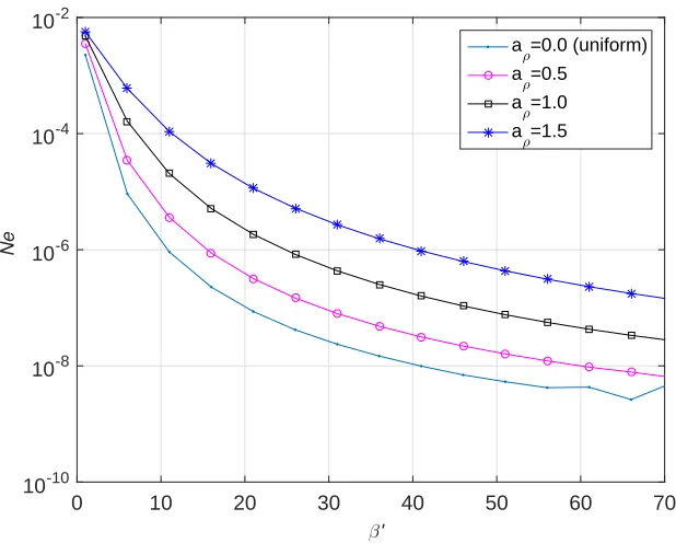
The ODEs are solved on a set of uniform (aρ = 0) and non-uniform (aρ ={0.5,1.0, 1.5}) grids with different sizes N ={101,201, ...,1001}. For ODE-1, its solution accuracy (Ne) against the RBF width (β′) is presented
in Fig.2(forN = 501) while the behaviour ofNeagainst the number of grid nodes is presented in Fig.3(forβ′ = 50). The corresponding results for
ODE-2 are given in Figs.4and 5. The four figures show that the present approach yields greater accuracy for uniform grids (aρ= 0) and the accuracy increases as aρ is reduced. We will use uniform grids for the following computations.
4.2. Poisson equation
4.2.1. Poisson equation in a square domain:
In order to study the spatial accuracy of the present CIRBF approxima-tion scheme, we consider the following Poisson equaapproxima-tion
∂2u ∂x2 +
∂2u
∂y2 =−18π
2sin(3πx) sin(3πy), (4.52)
subject to the Dirichlet boundary condition derived from the following exact solution
in which 0 ≤x, y ≤ 1. The calculations are carried out on a set of uniform grids of {21×21,31×31, ...,71×71}. Table 1 gives comparison of numeri-cal solutions showing that the proposed scheme outperforms the higher order compact finite difference (HOC) scheme [34], 1D-IRBF [12] and finite differ-ence method with central-differdiffer-ence (FDM) scheme. The convergdiffer-ence rate is
O(g2.036) for the FDM scheme, O(g3.052) for the 1D-IRBF scheme, O(g4.837)
for the HOC scheme, and O(g4.847) for the present scheme.
To compare the computational cost of the CIRBF, 1D-IRBF and HOC schemes, we let the grid size increase as {21×21,22×22, ...} until the so-lution accuracy achieves a target RMS level of 10−5. Fig. 6 shows that the
present scheme takes much less time to reach the target accuracy than the 1D-IRBF and the HOC. It is noted that the final grid size used to achieve the target accuracy is 81×81 for the 1D-IRBF, 45×45 for the HOC, and 44×44 for the present CIRBF. Fig. 7 presents the RMS of the approxi-mate solutionuagainst the RBF width parameterβ′ for three different grids
(31×31,51×51 and 71×71). The solution accuracy becomes better as β′
increases to a certain value (β′ = 10 for the 31×31 grid, β′ = 20 for the
51×51 grid, andβ′ = 30 for the 71×71 grid) and beyond that the accuracy
is almost unchanged.
4.2.2. Poisson equation in a square domain with a circular hole:
The present method is also verified through the solution of the following 2D Poisson equation
∂2u ∂x2 +
∂2u
∂y2 =−8π
2sin(2πx) sin(2πy), (4.54)
defined on a non-rectangular domain as shown in Fig.8and subject to Dirich-let boundary conditions. The problem has the following exact solution
u= sin(2πx) sin(2πy), (4.55)
from which the boundary values of ucan be derived.
Fig.9presents the grid convergence study for the present CIRBF method in comparison with that of the 1D-IRBF and MLS-1D-IRBF methods [26]. The numerical results show that the present method yields more accurate solutions than its counterparts and has a higher convergence rate (error norm of O(g4.12)) than the 1D-IRBF (error norm of O(g3.00)) and the
of the approximate solution uagainst the RBF width parameter β′ for three
different grids. It can be seen that the optimal value ofβ′ varies with different
grids (i.e., β′ = 3 for the 25×25 grid, β′ = 6 for the 49×49 grid, andβ′ = 10
for the 73×73 grid). And, for a given grid size, the solution accuracy is almost unchanged with large values of β′. When solving arbitrary problems
which do not have analytical solutions, it could be difficult to determine the optimal RBF width. In those problems, we suggest to chooseβ′ large enough
(e.g., β′ = 15) to obtain stable and accurate numerical results.
4.3. Taylor-Green vortex
The Taylor-Green vortex is modelled by the incompressible transient Navier-Stokes equations written in the dimensionless non-conservative forms as
∂u ∂x +
∂v
∂y = 0, (4.56)
∂u ∂t +u
∂u ∂x +v
∂u ∂y =−
∂p ∂x +
1 Re
∂2u ∂x2 +
∂2u ∂y2
, (4.57)
∂v ∂t +u
∂v ∂x +v
∂v ∂y =−
∂p ∂y +
1 Re
∂2v ∂x2 +
∂2v ∂y2
, (4.58)
where u, v and pare velocity components in x-, y-direction and static pres-sure, respectively; Re =Ul/ν the Reynolds number, in whichν,l and U are the kinematic viscosity, characteristic length and characteristic speed of the flow, respectively. Consider Eqs. (4.56)–(4.58) with the initial condition
u(x, y) = −cos(κx) sin(κy), (4.59)
v(x, y) = sin(κx) cos(κy), (4.60)
where 0≤x, y ≤2π and κ= 2. The analytic solution for this problem is
u(x, y, t) =−cos(κx) sin(κy) exp(−2κ2t/Re), (4.61)
v(x, y, t) = sin(κx) cos(κy) exp(−2κ2t/Re), (4.62) p(x, y, t) =−1/4{cos(2κx) + cos(2κy)}exp(−4κ2t/Re). (4.63)
CIRBF-Fully Coupled, is applied to solve this problem at Re = 100. A time step is taken to be ∆t = 0.002. The present numerical results are compared with those obtained by Tian et al. [34] who used the upwind HOC scheme based on a fractional step approach and a staggered grid system (HOC-Fractional). For the purpose of comparison, we also implement the HOC scheme [34] into the present fully coupled fluid solver, named as HOC-Fully Coupled. Table 2shows the accuracy comparison between the CIRBF-Fully Coupled, HOC-Fully Coupled and HOC-Fractional at time t = 2 for differ-ent grid sizes. It is seen that CIRBF-Fully Coupled approach yields much better accuracy and better convergence rates than the HOC-Fractional [34], and also performs better than the HOC-Fully Coupled. To investigate the computational efficiency of the CIRBF and HOC schemes when solving the time-dependent problem, we increase the grid size as {11×11,13×13, ...} until the solution accuracy of the u-velocity achieves a targetRMS level of 10−3. Fig.11shows that the present-CIRBF scheme reaches the target
accu-racy faster than the HOC approach. It is noted that the final grid size used to achieve the target accuracy is 29×29 for the HOC, 29×29 for the previous CIRBF, and 27×27 for the present CIRBF. We also compare the present CIRBF results with those of the previous CIRBF scheme presented by Tien et al. [32]. The numerical results show that the present scheme performs better than the previous scheme as shown in Fig. 11.
5. Numerical results and discussion
In this section, we apply the proposed numerical approach based on the CIRBF scheme and the rational function transformation (RFT) method to simulate 1–D moisture motions in homogeneous and layered soils and 2–D moisture motions in heterogeneous soils.
5.1. One-dimensional flow in a homogeneous soil
The performance of the proposed numerical approach is investigated through three different sets of soil properties as follows.
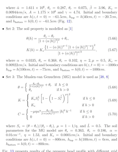
• Set 1: The soil property is modelled as [37]
θ(h) = αˆ(θs−θr) ˆ
α+|h|βˆ +θr, (5.64)
K(h) =Ks A
where ˆα = 1.611 × 10⁶, θ
s = 0.287, θr = 0.075, ˆβ = 3.96, Ks = 0.00944cm/s, A = 1.175 ×10⁶ and γ = 4.74. Initial and boundary
conditions are h(z, t = 0) = −61.5cm, htop = h(40cm, t) = −20.7cm, and hbottom =h(0, t) =−61.5cm(Fig. 12).
• Set 2: The soil property is modelled as [1]
θ(h) = θs−θr
[1 + (α|h|)η]µ +θr, (5.66)
K(h) =Ks
1−(α|h|)η−1[1 + (α|h|)η]−µ 2
[1 + (α|h|)η]µ/2 , (5.67) where α = 0.0335, θs = 0.368, θr = 0.102, η = 2, µ = 0.5, Ks = 0.00922cm/s. Initial and boundary conditions areh(z, t= 0) =−1000cm,
htop =h(100cm, t) =−75cm, and hbottom =h(0, t) = −1000cm. • Set 3: The Mualen-van Genuchten (MG) model is used as [38, 8]
θ =
θs−θr
[1+(α|h|)η]µ +θr if h≤0 θs if h >0
(5.68)
K =
KsSeLˆ
1−
1−S
1 µ
e µ2
ifh≤0
Ks ifh >0
(5.69)
C =
(
−µηαη θs−θr
[1+(α|h|)η]µ+1 |h| η
h−1 if h≤0
0 if h >0 (5.70)
where Se = (θ−θr)/(θs−θr), µ = 1 −1/η, and ˆL = 0.5. The soil parameters for the MG model are θs = 0.363, θr = 0.186, α = 0.01cm−1, η = 1.53, and K
s = 0.0001cm/s. Initial and boundary conditions are h(z, t = 0) = −800cm, htop = h(100cm, t) = 0cm, and hbottom =h(0, t) =−800cm.
[image:17.612.121.502.109.599.2]solutions obtained by the CIRBF method are in good agreement with the numerical result of Celia et al. [1] and the analytical result of Warrick et al. [38]. We investigate the effect of time step (∆t) on the solutions of the present method and compare the results with those presented by Celia et al. [1] for Set 2. The grid size is taken to be ∆z = 2.5cm. The time step is chosen as ∆t = 60.0, 12.0 and 2.4 minutes. Fig. 16 shows that the present results converge to the dense grid result of Celia et al. faster than those of the FDM when the time step reduces.
5.2. One-dimensional flow in a layered soil
The proposed method is applied to simulate flow in a layered soil for several cases with different values of initial pressure (h0) and vertical flux at the top of the soil column (qA) as shown in Table3. These cases are the same as the ones in the published works [2,3,6]. The soil profile has Soil 1 (Berino loamy fine sand) from 0 to 50cmand 90 to 100cm, and Soil 2 (Glendale clay loam) from 50 to 90cm. The hydraulic parameters of these soils based on the van Genuchten model are presented in Table4. The simulation time step (∆t) is determined based on an adaptive time-stepping scheme [39, 2] for efficiency and robustness. The time step is increased by 10% if the number of Picard iterations for the previous time step is less than 4 and decreased by 10% if the number of iterations is greater than 8. Fig. 17presents results of pressure head and volumetric water content with different grid resolutions for Case 1.1 using the FDM and CIRBF scheme. It can be seen that the CIRBF solution converges faster than that of the FDM. The obtained numerical results for all cases at a grid of 101 are in good agreement with those of the FDM and the FVM [6] as shown in Fig. 18.
5.3. Two-dimensional flow in a heterogeneous soil
We simulate the moisture motion in heterogeneous porous media in two dimensions as described in [2]. The computational domain and boundary conditions are illustrated in Fig. 19. All boundaries are non-flow (q= 0) ex-cept the segment of 100cmwide at the top where the vertical flux of 5cm/day
is applied. The computational region is divided into 9 alternating blocks of Sand and Clay. Sand and Clay are Berino loamy fine sand and Glendale clay loam, respectively.
We apply the proposed numerical approach to solve this problem. Fig.20
gives the vertical and horizontal fluxes at the cross sections x = 5cm and
−50× 103cm. It is observed that the current numerical results converge
to the dense grid solution obtained by the FDM [4] when refining the grid density. At the same grid size of 5cm, the present result is slightly more accurate than that of the FDM.
The present method is applied to solve the 2–D soil problem for several grid sizes of ∆x= ∆z ={5.0,6.25,10.0, 20.0, 25.0, 50.0}cm for the case of
h0 =−50×103cmto investigate how coarse the grid can be before the scheme
fails. It appears that the method can yield the solution until the grid size of 25.0cm(Figs. 21) and fails at the grid size of 50.0cm. Fig.22illustrates the contours of pressure head at 12.5 days with different grid resolutions of 10.0, 6.25 and 5.0 cm. Figs. 23-25 show the contour of pressure head at several time moments (t= 1.0, 6.0 and 12.5 days) for different initial pressure heads
h0 =−103cm,−15×103cmand −50×103cm, respectively.
For the purpose of CPU time comparisons, we implement the FDM+RFT method to solve the present 2-D soil problem and run all related computations on the same computer. Table 5 shows the CPU time and total number of Picard iterations required for the present CIRBF+RFT simulations in comparison with those of the FDM+RFT simulations. It can be seen that the FDM+RFT method requires less CPU times and number of Picard iterations than the present method.
6. Conclusions
A generalised finite difference approach based on the CIRBF method and the rational function transformation (RFT) method has been success-fully developed for simulating the fluid movement in homogeneous and het-erogeneous soils. The CIRBF method of a high level of accuracy and fast convergence rate has been demonstrated through the solution of a Poisson equation and a Taylor-Green vortex. When solving the Poisson equation in a non-rectangular domain, the present method performs better than its coun-terparts (1D-IRBF and MLS-1D-IRBF). The enhanced convergence rate of the present scheme provides an ability to obtain prescribed accuracy faster than the 1D-IRBF and HOC schemes. The numerical results for Poisson equations indicate that the RBF-width parameter β′ should be chosen large
enough to get high accurate solutions. The value of β′ is taken to be 15.0
The CIRBF numerical results obtained for different initial and boundary conditions are in good agreement with other published results in the liter-ature. However, the CIRBF+RFT method consumes more CPU time than the FDM+RFT method because it requires more CPU time for construct-ing the CIRBF interpolation matrix. Therefore, further study is needed to improve the present scheme in order to reduce the computational cost for solving soil problems.
Acknowledgement
Dr D. Ngo-Cong, Dr T. Nguyen-Ky and Dr D.-A. An-Vo are Vice-Chancellor’s Research Fellows and would like to thank the University of Southern Queens-land for the support through the University’s Strategic Research Fund ini-tiative. The authors would like to thank the reviewers for their helpful com-ments.
References
[1] Celia MA, Bouloutas ET, Zarba RL. A general mass-conservative numer-ical solution for the unsaturated flow equation.Water Resources Research
1990; 26 (7):483–1496.
[2] Kirkland MR, Hills RG, Wierenga PJ. Algorithms for solving Richards’ equation for variably saturated soils. Water Resources Research 1992; 28:2049–2058.
[3] Pan L, Wierenga PJ. A transformed pressure head-based approach to solve Richards’ equation for variably saturated soils. Water Resources Research 1995; 31(4):925–931.
[4] Pan L, Wierenga PJ. Improving numerical modeling of two-dimensional water flow in variably saturated, heterogenous porous media.Soil Science Society of America Journal 1997; 61(2):335–346.
[5] Forsyth PA, Wu YS, Pruess K. Robust numerical methods for saturated– unsaturated flow with dry initial conditions in heterogeneous media. Ad-vances in Water Resources 1995; 18:25–38.
[7] Zambra CE, Dumbser M, Toro EF, Moraga NO. A novel numerical method of high-order accuracy for flow in unsaturated porous media. In-ternational Journal for Numerical Methods in Engineering 2012; 89:227– 240.
[8] Caviedes-Voulli`eme D, Garc´ıa-Navarro P, Murillo J. Verification, con-servation, stability and efficiency of a finite volume method for the 1D Richards equation. Journal of Hydrology 2013; 480:69–84.
[9] Madych WR, Nelson SA. Multivariate interpolation and conditionally positive definite functions. Approximation Theory and its Applications
1989; 4:77–89.
[10] Kansa EJ. Multiquadrics - A scattered data approximation scheme with applications to computational fulid-dynamics - I: Surface approximations and partial derivative estimates. Computers & Mathematics with Appli-cations 1990; 19(8–9):127–145.
[11] Mai-Duy N, Tran-Cong T. Numerical solution of differential equations using multiquadric radial basis function networks.Neural Networks 2001; 14:185–199.
[12] Mai-Duy N, Tanner RI. A collocation method based on one-dimensional RBF interpolation scheme for solving PDEs. International Journal of Numerical Methods for Heat & Fluid Flow 2007; 17(2):165–186.
[13] Zerroukat M, Djidjeli K, Charafi A. Explicit and implicit meshless meth-ods for linear advection-diffusion-type partial differential equations. Inter-national Journal for Numerical Methods in Engineering 2000; 48:19–35. [14] Lee CK, Liu X, Fan SC. Local multiquadric approximation for solving
boundary value problems. Computational Mechanics 2003; 30:396–409. [15] Shu C, Ding H, Yeo KS. Local radial basis function-based differential
quadrature method and its application to solve two-dimensional incom-pressible Navier-Stokes equations.Computer Methods in Applied Mechan-ics and Engineering 2003; 192:941–954.
[17] Wright GB, Fornberg B. Scattered node compact finite difference-type formulas generated from radial basis functions.Journal of Computational Physics 2006; 212:99–123.
[18] Fornberg B, Lehto E. Stabilization of RBF-generated FDMs for convec-tive PDEs. Journal of Computational Physics 2011; 230:2270–2285. [19] Flyer N, Fornberg B, Bayona V, Barnett GA. On the role of polynomials
in RBF-FD approximations: I. Interpolation and accuracy. Journal of
Computational Physics 2016; 321:21–38.
[20] Vertnik R, ˇSarler B. Meshless local radial basis function collocation method for convective-diffusive solid-liquid phase change problems. In-ternational Journal of Numerical Methods for Heat & Fluid Flow 2006; 16:617–640.
[21] Stevens D, Power H, Lees M, Morvan H. The use of PDE centres in the local RBF Hermitian method for 3D convective-diffusion problems.
Journal of Computational Physics 2009; 228:4606–4624.
[22] Jackson SJ, Stevens D, Giddings D, Power H. An adaptive RBF finite collocation approach to track transport processes across moving fronts.
Computers & Mathematics with Applications 2016; 71(1):278–300. [23] An-Vo DA, Mai-Duy N, Tran-Cong T. A C2-continuous control-volume
technique based on cartesian grids and two-node integrated-rbf elements for second-order elliptic problems.Computer Modeling in Engineering & Sciences 2011; 72(4):299–334.
[24] An-Vo DA, Mai-Duy N, Tran-Cong T. High-order upwind methods based on C 2-continuous two-node integrated-RBF elements for viscous flows. Computer Modeling in Engineering & Sciences 2011; 80 (2):141– 177.
[25] An-Vo DA, Tran C-D, Mai-Duy N, Tran-Cong T. RBF-based multiscale control volume method for second order elliptic problems with oscilla-tory coefficients. Computer Modeling in Engineering & Sciences 2012; 89(4):303–359.
Viscous Flows. International Journal for Numerical Methods in Fluids
2012; 70:1443–1474.
[27] Mai-Duy N, Tran-Cong T. Compact local integrated-RBF approxima-tions for second-order elliptic differential problems.Journal of Computa-tional Physics 2011; 230:4772–4794.
[28] Mai-Duy N, Tran-Cong T. A compact five-point stencil based on inte-grated RBFs for 2D second-order differential problems. Journal of Com-putational Physics 2013; 235:302–321.
[29] Thai-Quang N, Le-Cao K, Mai-Duy N, Tran C-D, Tran-Cong T. A numerical scheme based on compact integrated-RBFs and Adams-Bashforth/Crank-Nicolson algorithms for diffusion and unsteady fluid flow problems. Engineering Analysis with Boundary Elements 2013; 37(12):1653–1667.
[30] Hardy RL. Theory and applications of the multiquadric-biharmonic method.Computers & Mathematics with Applications 1990; 8-9:163–208. [31] Sarra SA. Integrated multiquadric radial basis function approximation methods. Computers & Mathematics with Applications 2006; 51:1283– 1296.
[32] Tien CMT, Thai-Quang N, Mai-Duy N, Tran C-D, Tran-Cong T. High-order fully coupled scheme based on compact integrated RBF approx-imation for viscous flows in regular and irregular domains. Computer Modeling in Engineering & Sciences 2015; 105:301–340.
[33] Ngo-Cong D, Mai-Duy N, Karunasena W, Tran-Cong T. Local Moving Least Square - One-Dimensional IRBFN Technique: Part I - Natural Con-vection Flows in Concentric and Eccentric Annuli.Computer Modeling in Engineering & Sciences 2012; 83(3): 275–310.
[34] Tian Z, Liang X, Yu P. A higher order compact finite difference algo-rithm for solving the incompressible Navier Stokes equations. Interna-tional Journal for Numerical Methods in Engineering 2011; 88:511–532. [35] Hanby RF, Silvester DJ, Chew JW. A comparison of coupled and
[36] Mazhar Z. A procedure for the treatment of the velocity-pressure cou-pling problem in incompressible fluid flow.Numerical Heat Transfer, Part B: Fundamentals: An International Journal of Computation and Method-ology 2001; 39(1):91–100.
[37] Haverkamp R, Vauclin M, Touma J, Wierenga PJ, Vachaud G. A com-parison of numerical simulation models for one-dimensional infiltration.
Soil Science Society of America Journal 1977; 41:285–294.
[38] Warrick AW, Lomen DO, Yates SR. A generalized solution to infiltra-tion. Soil Science Society of America Journal 1985; 49(1):34–38.
Table 1: Poisson equation: grid convergence study ofRM Sfor the present CIRBF method (β′ = 25) in comparison with the FDM, 1D-IRBF and HOC methods.
Grid FDM 1D-IRBF HOC Present CIRBF
21×21 8.9109E-03 5.8623E-04 3.3579E-04 3.3220E-04 31×31 3.9994E-03 1.7845E-04 5.6856E-05 5.5507E-05 41×41 2.2630E-03 7.6214E-05 1.4589E-05 1.4036E-05 51×51 1.4540E-03 3.9174E-05 4.9330E-06 4.6891E-06 61×61 1.0125E-03 2.2653E-05 2.0151E-06 1.9215E-06 71×71 7.4536E-04 1.4215E-05 9.4467E-07 9.4341E-07 Convergence rate O(g2.036) O(g3.052) O(g4.837) O(g4.847)
Table 2: Taylor-Green vortex: grid convergence study of numerical results at t= 2.0 for the present CIRBF-Fully Coupled (β′= 15) in comparison with the HOC-Fully Coupled
and HOC-Fractional [34].
Present CIRBF-Fully Coupled
Grid u-error v-error p-error
11×11 1.5214251E-01 1.5218216E-01 5.3403483E-01 21×21 3.9925074E-03 3.9924747E-03 2.1199636E-02 31×31 3.2600624E-04 3.2600469E-04 5.1768763E-03 41×41 2.8866736E-05 2.8866407E-05 6.0032401E-04 51×51 1.4292601E-05 1.4292574E-05 4.2213874E-04 Rate O(g5.96
) O(g5.96
) O(g4.56 ) HOC-Fully Coupled
Grid u-error v-error p-error
11×11 1.8156049E-01 1.8156049E-01 3.0412542E-01 21×21 4.5719207E-03 4.5719207E-03 8.5425929E-03 31×31 5.0521189E-04 5.0521191E-04 2.6558403E-03 41×41 1.0478762E-04 1.0478758E-04 3.4579194E-04 51×51 3.0814364E-05 3.0814437E-05 2.6395965E-04 Rate O(g5.39
) O(g5.39
) O(g4.47 ) HOC-Fractional [34]
Grid u-error v-error p-error
11×11 7.0070489E-02 7.0070489E-02 1.0764149E-01 21×21 9.0692193E-03 9.0692193E-03 1.0567607E-02 31×31 2.8851487E-03 2.8851487E-03 2.9103288E-03 41×41 1.2238736E-03 1.2238736E-03 1.1356134E-03 51×51 6.3063026E-04 6.3063026E-04 5.3933641E-04 Rate O(g2.92
) O(g2.92
[image:25.612.168.441.358.654.2]Table 3: One-dimensional flow in a layered soil: initial and boundary conditions, elapsed times. h0 is the initial pressure, andqAandqCdenote for the vertical flux at the top and bottom of the soil column, respectively.
Case h0(cm) qA(cm/h) qC(cm/h) Elapsed time (h)
1.1 -200 0.3 0 4.0
1.2 -1000 0.3 0 8.0
1.3 -50000 0.3 0 12.0
2.1 -200 1.25 0 3.8
2.2 -1000 1.25 0 5.0
2.3 -50000 1.25 0 6.0
Table 4: Hydraulic parameters of Soils 1 and 2 in a layered soil.
Parameters Soil 1 Soil 2
θs 0.3658 0.4686
θr 0.0286 0.1060
α(cm−1
) 0.0280 0.0104 ˆ
η 2.2390 1.3954
[image:26.612.235.378.519.595.2]Table 5: 2-D soil problem: comparisons (between the present CIRBF+RFT and FDM+RFT) of CPU time and total number of Picard iterations (Niteration) required for simulations with different initial pressure heads (h0) and several grid sizes (∆x= ∆z).
h0(cm) Method Grid size (cm) CPU time (s) Niteration
-1000 FDM+RFT 20.00 17.2 1449
10.00 301.3 2362
6.25 2910.9 3845
5.00 8776.6 4876
CIRBF+RFT 20.00 68.1 2514
10.00 2296.0 5459
6.25 28481.1 10057
5.00 107098.0 13278
-15000 FDM+RFT 20.00 18.7 1497
10.00 290.6 2381
6.25 3389.7 4044
5.00 9235.0 4995
CIRBF+RFT 20.00 70.0 2595
10.00 2380.3 5584
6.25 32343.2 10333
5.00 110045.6 13520
-50000 FDM+RFT 20.00 17.5 1230
10.00 284.6 2571
6.25 3345.1 4130
5.00 7841.0 5110
CIRBF+RFT 20.00 79.7 2639
10.00 2100.5 5750
6.25 30612.9 9579
β'
0 10 20 30 40 50 60 70
Ne
10-10
10-8
10-6
10-4
10-2
aρ=0.0 (uniform) a
ρ=0.5
[image:29.612.152.461.250.498.2]aρ=1.0 aρ=1.5
Fig. 2: ODE-1: the solution accuracy (N e) against the RBF width (β′) for four different
Number of nodes N
200 300 400 500 600 700 800 900 1000
Ne
10-9
10-8
10-7
10-6
10-5
10-4
aρ=0.0 (uniform) aρ=0.5
[image:30.612.152.459.250.500.2]aρ=1.0 aρ=1.5
β'
0 10 20 30 40 50 60 70
Ne
10-10
10-8
10-6
10-4
10-2
aρ=0.0 (uniform) aρ=0.5
[image:31.612.153.461.250.495.2]aρ=1.0 aρ=1.5
Fig. 4: ODE-2: the solution accuracy (N e) against the RBF width (β′) for four different
Number of nodes N
200 300 400 500 600 700 800 900 1000
Ne
10-9
10-8
10-7
10-6
10-5
aρ=0.0 (uniform) aρ=0.5
[image:32.612.153.459.252.500.2]aρ=1.0 aρ=1.5
CPU Time (second)
10-1 100 101 102
RMS
10-5
10-4
10-3
1D-IRBF HOC
[image:33.612.154.464.237.490.2]present CIRBF
Fig. 6: Poisson equation: comparison of computational cost of the present CIRBF, 1D-IRBF and HOC schemes. The grid size increases as{21×21,22×22, ...}until the solution accuracy achieves a targetRM Slevel of 10−5
0 10 20 30 40 50 60 70 10−7
10−6 10−5 10−4 10−3 10−2
β’
RMS
[image:34.612.154.459.254.497.2]grid 31×31 grid 51×51 grid 71×71
Fig. 7: Poisson equation: the solution accuracy (RM S) against the RBF width (β′) for
−2 −1 0 1 2 −2
−1.5 −1 −0.5 0 0.5 1 1.5 2
x
[image:35.612.198.416.272.486.2]y
10-2 10-1 h
10-6
10-5
10-4
10-3
10-2
10-1
Ne
1D-IRBF, O(g3.00)
MLS-1D-IRBF, O(g3.70)
[image:36.612.154.463.249.501.2]Present CIRBF, O(g4.12)
0 10 20 30 40 50 60 70
10−4
10−3
10−2
10−1
β’
Ne
grid 25×25
grid 49×49
[image:37.612.154.458.250.498.2]grid 73×73
CPU Time (second)
100 101 102
RMS
10-4
10-3
10-2
10-1
100
HOC-Fully Coupled
[image:38.612.154.460.239.487.2]previous CIRBF-Fully Coupled present CIRBF-Fully Coupled
Fig. 11: Taylor-Green vortex: comparison of computational cost of the present CIRBF and HOC schemes. The grid size increases as{11×11,13×13, ...}until the solution accuracy of the u-velocity achieves a targetRM S level of 10−3
−800 −70 −60 −50 −40 −30 −20 5
10 15 20 25 30 35 40
h(cm)
Depth
z(cm)
[image:40.612.139.473.263.541.2]CIRBF,nz=31 CIRBF,nz=41 CIRBF,nz=81 CIRBF,nz=101 CIRBF,nz=201 FDM, Celia et al.
−1000 −800 −600 −400 −200 0 0
10 20 30 40 50 60 70 80 90 100
h(cm)
Depth
z(cm)
[image:41.612.138.474.240.509.2]CIRBF,nz=51 CIRBF,nz=101 CIRBF,nz=201 CIRBF,nz=301 CIRBF,nz=401 FDM, Celia et al.
−800 −600 −400 −200 0 0
10 20 30 40 50 60 70 80 90 100
h(cm)
Depth
z(cm)
CIRBF,nz=51 CIRBF,nz=101 CIRBF,nz=141 CIRBF,nz=161 CIRBF,nz=201
[image:42.612.139.473.243.505.2]Analytical, Warrick et al.
-1000 -800 -600 -400 -200 0 h(cm)
0 20 40 60 80 100
Depth
z(cm)
FDM, Celia et al., time step=60.0min FDM, Celia et al., time step=12.0min FDM, Celia et al., time step=2.4min FDM, Celia et al., dense grid
(a)
-1000 -800 -600 -400 -200 0
h(cm) 0
20 40 60 80 100
Depth
z(cm)
CIRBF+RFT, time step=60.0min CIRBF+RFT, time step=12.0min CIRBF+RFT, time step=2.4min FDM, Celia et al., dense grid
[image:43.612.140.476.126.653.2]−220 −200 −180 −160 −140 −120 −1000 −80 −60 20
40 60 80 100
h(cm)
z(cm)
FDM, grid 51 FDM, grid 101 FDM, grid 151 FDM, grid 201
0.050 0.1 0.15 0.2 0.25 0.3 0.35 0.4 20
40 60 80 100
θ
z(cm)
FDM, grid 51 FDM, grid 101 FDM, grid 151 FDM, grid 201
FVM, McBride et al., 100 elements
−220 −200 −180 −160 −140 −120 −1000 −80 −60 20
40 60 80 100
h(cm)
z(cm)
CIRBF, grid 51 CIRBF, grid 101 CIRBF, grid 151 CIRBF, grid 201
0.050 0.1 0.15 0.2 0.25 0.3 0.35 0.4 20
40 60 80 100
θ
z(cm)
CIRBF, grid 51 CIRBF, grid 101 CIRBF, grid 151 CIRBF, grid 201
[image:44.612.208.404.118.765.2]qA= 0.3cm/h qA = 1.25cm/h
0 0.05 0.1 0.15 0.2 0.25 0.3 0.35 0.4 0.45
0 10 20 30 40 50 60 70 80 90 100 θ z(cm) FDM, h
A= −200cm
FDM, h
A= −1000cm
FDM, h
A= −50000cm
FVM, McBride et al., h
A= −200cm
FVM, McBride et al., h
A= −1000cm
FVM, McBride et al., h
A= −50000cm
0 0.1 0.2 0.3 0.4 0.5
0 10 20 30 40 50 60 70 80 90 100 θ z(cm) FDM, h
A= −200cm
FDM, hA= −1000cm
FDM, h
A= −50000cm
FVM, McBride et al., hA= −200cm
FVM, McBride et al., h
A= −1000cm
FVM, McBride et al., hA= −50000cm
0 0.05 0.1 0.15 0.2 0.25 0.3 0.35 0.4 0.45
0 10 20 30 40 50 60 70 80 90 100 θ z(cm) CIRBF, h
A= −200cm
CIRBF, h
A= −1000cm
CIRBF, h
A= −50000cm
FVM, McBride et al., h
A= −200cm
FVM, McBride et al., h
A= −1000cm
FVM, McBride et al., h
A= −50000cm
10 20 30 40 50 60 70 80 90 100 z(cm)
CIRBF, hA= −200cm
CIRBF, h
A= −1000cm
CIRBF, hA= −50000cm
FVM, McBride et al., h
A= −200cm
FVM, McBride et al., hA= −1000cm
−300 −250 −200 −150 −100 −50 0 −8
−7 −6 −5 −4 −3 −2 −1 0 1
z (cm)
q
z
(cm/day)
Present, grid size=25.00cm Present, grid size=20.00cm Present, grid size=10.00cm Present, grid size=6.25cm Present, grid size=5.00cm
FDM, Pan & Wierenga, grid size=5cm FDM, Pan & Wierenga, dense grid
−200 −100 0 100 200
−2 0 2 4 6
x (cm)
q
x
(cm/day)
Present, grid size=25.00cm Present, grid size=20.00cm Present, grid size=10.00cm Present, grid size=6.25cm Present, grid size=5.00cm
[image:47.612.179.431.152.574.2]FDM, Pan & Wierenga, grid size=5cm FDM, Pan & Wierenga, dense grid
Fig. 20: 2-D soil problem: results of vertical flux qz at x = 5cm(top) and horizontal flux qx at y = 95cm (bottom) for several grid resolutions, at time t = 12.50 days, for
h0 = −50×10 3
−40000
−40000 −40000
−40000
−200
−200 −200
−200
−100 −100
−100
−60
−60
x (cm)
z (cm)
−200 −100 0 100 200
−300 −250 −200 −150 −100 −50 0
[image:48.612.181.430.294.446.2]Grid size=25.00cm Grid size=20.00cm Grid size=10.00cm
Fig. 21: 2-D soil problem: contours of pressure head h(cm) att = 12.50 days, using the CIRBF scheme in conjunction with the RFT method, and different grid sizes ∆x= ∆z=
{25,20,10}cm, forh0=−50×10 3
−900 −900 −900 −900 −900 −200 −200 −200 −200 −100 −100 −100 −100 −60 −60 −60 x (cm) z (cm) h
0=−1000 cm
−200 −100 0 100 200
−300 −250 −200 −150 −100 −50 0 Grid size=10.00cm Grid size=6.25cm Grid size=5.00cm −14000 −14000 −14000 −14000 −200 −200 −200 −200 −100 −100 −100 −60 −60 x (cm) z (cm) h
0=−15000 cm
−200 −100 0 100 200
−300 −250 −200 −150 −100 −50 0 Grid size=10.00cm Grid size=6.25cm Grid size=5.00cm −40000 −40000 −40000 −40000 −200 −200 −200 −200 −100 −100 −100 −60 −60 x (cm) z (cm) h
0=−50000 cm
−200 −100 0 100 200
[image:49.612.179.431.125.647.2]−300 −250 −200 −150 −100 −50 0 Grid size=10.00cm Grid size=6.25cm Grid size=5.00cm
−900 −900 −200 −100 x (cm) z (cm)
At t = 1.00 days
−200 −100 0 100 200
−300 −250 −200 −150 −100 −50 0 −900 −900 −900 −200 −200 −200 −100 −100 −100 x (cm) z (cm)
At t = 6.00 days
−200 −100 0 100 200
−300 −250 −200 −150 −100 −50 0 −900 −900 −900 −900 −900 −200 −200 −200 −200 −100 −100 −100 −100 −60 −60 −60 x (cm) z (cm)
At t = 12.50 days
−200 −100 0 100 200
[image:50.612.178.433.128.635.2]−300 −250 −200 −150 −100 −50 0
Fig. 23: 2-D soil problem: contours of pressure head h(cm) at different times t forh0=
−103
−14000 −14000 −200 −100 x (cm) z (cm)
At t = 1.00 days
−200 −100 0 100 200
−300 −250 −200 −150 −100 −50 0 −14000 −14000 −14000 −200 −200 −200 −100 −100 −100 x (cm) z (cm)
At t = 6.00 days
−200 −100 0 100 200
−300 −250 −200 −150 −100 −50 0 −14000 −14000 −14000 −14000 −200 −200 −200 −200 −100 −100 −100 −60 −60 x (cm) z (cm)
At t = 12.50 days
−200 −100 0 100 200
[image:51.612.179.432.127.636.2]−300 −250 −200 −150 −100 −50 0
Fig. 24: 2-D soil problem: contours of pressure head h(cm) at different times t forh0=
−15×103
−40000 −40000 −200 −100 x (cm) z (cm)
At t = 1.00 days
−200 −100 0 100 200
−300 −250 −200 −150 −100 −50 0 −40000 −40000 −40000 −200 −200 −200 −100 −100 −100 x (cm) z (cm)
At t = 6.00 days
−200 −100 0 100 200
−300 −250 −200 −150 −100 −50 0 −40000 −40000 −40000 −40000 −200 −200 −200 −200 −100 −100 −100 −60 −60 x (cm) z (cm)
At t = 12.50 days
−200 −100 0 100 200
[image:52.612.179.432.128.635.2]−300 −250 −200 −150 −100 −50 0
Fig. 25: 2-D soil problem: contours of pressure head h(cm) at different times t forh0=
−50×103