The evolution of surface magnetic fields in young solar-type stars I: the first 250 Myr

(1)

The evolution of surface magnetic fields in young solar-type stars – I.

The first 250 Myr

⋆

C. P. Folsom,

1,2

_†

_{P. Petit,}

3,4

_{J. Bouvier,}

1,2

_{A. L`ebre,}

5

_{L. Amard,}

5

_{A. Palacios,}

5

J. Morin,

5

_{J.-F. Donati,}

3,4

_{S. V. Jeffers,}

6

_{S. C. Marsden}

7

_{and A. A. Vidotto}

8

1_{Universit´e Grenoble Alpes, IPAG, F-38000 Grenoble, France} 2_{CNRS, IPAG, F-38000 Grenoble, France}

3_{Universit´e de Toulouse, UPS-OMP, IRAP, F-31400 Toulouse, France}

4_{CNRS, Institut de Recherche en Astrophysique et Planetologie, 14, avenue Edouard Belin, F-31400 Toulouse, France} 5_{LUPM, Universit´e de Montpellier, CNRS, Place Eug`ene Bataillon, F-34095, France}

6_{Institut für Astrophysik, Georg-August-Universität Göttingen, Friedrich-Hund-Platz 1, D-37077 Göttingen, Germany}

7_{Computational Engineering and Science Research Centre, University of Southern Queensland, Toowoomba, QLD 4350, Australia} 8_{Observatoire de Genève, Université de Genève, Chemin des Maillettes 51, CH-1290 Versoix, Switzerland}

Accepted 2015 December 11. Received 2015 December 8; in original form 2015 September 17

ABSTRACT

The surface rotation rates of young solar-type stars vary rapidly with age from the end of the pre-main sequence through the early main sequence. Important changes in the dynamos operating in these stars may result from this evolution, which should be observable in their surface magnetic fields. Here we present a study aimed at observing the evolution of these magnetic fields through this critical time period. We observed stars in open clusters and stellar associations of known ages, and used Zeeman Doppler imaging to characterize their complex magnetic large-scale fields. Presented here are results for 15 stars, from five associations, with ages from 20 to 250 Myr, masses from 0.7 to 1.2 M_⊙, and rotation periods from 0.4 to 6 d. We find complex large-scale magnetic field geometries, with global average strengths from 14 to 140 G. There is a clear trend towards decreasing average large-scale magnetic field strength with age, and a tight correlation between magnetic field strength and Rossby number. Comparing the magnetic properties of our zero-age main-sequence sample to those of both younger and older stars, it appears that the magnetic evolution of solar-type stars during the pre-main sequence is primarily driven by structural changes, while it closely follows the stars’ rotational evolution on the main sequence.

Key words: techniques: polarimetric – stars: formation – stars: imaging – stars: magnetic field – stars: rotation – stars: solar-type.

1 I N T RO D U C T I O N

Solar-type stars undergo a dramatic evolution in their rotation rates as they leave the pre-main sequence (PMS) and settle into the main sequence (MS; for a recent review see Bouvier2013). Early on the PMS stellar rotation rates are regulated, likely due to interactions between a star and its disc. Eventually, after a few Myr, solar-type

⋆_{Based on observations obtained at the Canada–France–Hawaii Telescope} (CFHT), which is operated by the National Research Council of Canada, the Institut National des Sciences de l’Univers of the Centre National de la Recherche Scientifique of France, and the University of Hawaii. Also based on observations obtained at the Télescope Bernard Lyot (TBL, Pic du Midi, France) of the Midi-Pyrénées Observatory, which is operated by the Institut National des Sciences de l’Univers of the Centre National de la Recherche Scientifique of France.

†E-mail:folsomc@ujf-grenoble.fr

stars decouple from their discs and around this time the disc begins dissipating. Since the stars are still contracting on the PMS, they spin up. On a slower time-scale, solar-type stars lose angular mo-mentum through a magnetized wind. Thus once a star has reached the MS it begins to spin down (e.g. Schatzman1962; Skumanich 1972; Mestel & Spruit1987). Since solar-type stars have dynamo-driven magnetic fields, there is likely an important evolution in their magnetic properties over this time period. Such changes in magnetic properties could be driven both by changes in rotation rate and by changes in the internal structure of PMS stars (e.g. Gregory et al. 2012). In turn, stellar magnetic fields play a key role in angular mo-mentum loss. Thus understanding these magnetic fields is critical for understanding the rotational evolution of stars (e.g. Vidotto et al. 2011; Matt et al.2012; R´eville et al.2015).

Rotation rates deeper in a star may differ somewhat from this description of observed surface rotation rates. During the spin-down phase angular momentum is lost from the surface of a star,

at University of Southern Queensland on March 27, 2016

http://mnras.oxfordjournals.org/

(2)

potentially creating enhanced radial differential rotation. Recent ro-tational models by Gallet & Bouvier (2013,2015) use differences between the core and envelope rotation rates to explain the evolution of observed surface rotation rates. These models predict a period of greatly enhanced radial differential rotation as a star reaches the MS. Other models of the rotational evolution of stars also have im-portant impacts on the magnetic properties of these stars, such as the ‘Metastable Dynamo Model’ of Brown (2014).

The large-scale magnetic fields of MS solar-type stars were first observed in detail many years ago (e.g. Donati & Collier Cameron 1997), and more recently the magnetic strengths and geometries of these stars have been characterized for a significant sample of these stars (e.g. Petit et al.2008). Some trends are apparent: there are clearly contrasting magnetic properties between solar-like stars and M-dwarfs (Morin et al.2008,2010). There is some evidence for a correlation between more poloidal magnetic geometries and slow rotation rates (Petit et al.2008). With a large sample of stars, there appears to be trends in large-scale magnetic field strength with age and rotation (Vidotto et al.2014). Zeeman broadening measure-ments from Saar (1996) and Reiners, Basri & Browning (2009) find trends in the small-scale magnetic field strength with rotation and Rossby number, particularly for M-dwarfs. Donati & Landstreet (2009) provide a detailed review of magnetic properties for a wide range of non-degenerate stars. Currently, the BCool collaboration is carrying out the largest systematic characterization of magnetic fields in MS solar-type stars, with early results in Marsden et al. (2014) and Petit et al. (in preparation).

On the PMS, large-scale magnetic fields have been observed and characterized for a large number of stars (e.g. Donati et al.2008a, 2010,2011a). These observations are principally from the ‘Mag-netic Protostars and Planets’ (MaPP) and ‘Mag‘Mag-netic Topologies of Young Stars and the Survival of massive close-in Exoplanets’ (MaTYSSE) projects. There are clear differences between the mag-netic properties of T Tauri stars (TTS) and older MS stars, which seem to be a consequence of the internal structure of the star (Gre-gory et al.2012). This appears to be similar to the difference between MS solar mass stars and M-dwarfs (Morin et al.2008).

We aim to provide the first systematic study of the magnetic properties of stars from the late PMS through the zero-age main sequence (ZAMS) up to∼250 Myr. This covers the most dramatic portion of the rotational evolution of solar mass stars. Observations of a few individual stars in this age and mass range have been made (e.g. HD 171488, Jeffers & Donati2008; Jeffers et al.2011; HD 141943, Marsden et al.2011; HD 106506, Waite et al.2011; HN Peg, Boro Saikia et al.2015; HD 35296 and HD 29615, Waite et al.2015), but to date only a modest number of stars have been observed on an individual basis.

In this paper we focus on young (not accreting) stars, in the age range 20–250 Myr, and in the restricted mass range from 0.7 to 1.2 M_⊙. This fills the gap between the TTS observations of MaPP and MaTYSSE and the older MS observations of BCool. The observations focus on stars in young clusters and associations, in order to constrain stellar ages. Spectropolarimetric observations and Zeeman Doppler imaging (ZDI) are used to determine the strength and geometry of the large-scale stellar magnetic fields. This work is being carried out as part of the ‘TOwards Understanding the sPIn Evolution of Stars’ (TOUPIES) project.1_{Observations are ongoing} in the large programme ‘History of the Magnetic Sun’ (HMS) at the Canada–France–Hawaii Telescope (CFHT). Future papers in this

1_{http://ipag.osug.fr/Anr_Toupies/}

series will expand the size of the sample, and extend the age range up to 600 Myr.

2 O B S E RVAT I O N S

We obtained time series of spectropolarimetric observations using the ESPaDOnS instrument at the CFHT (Donati 2003; see also Silvester et al.2012), and the Narval instrument (Aurière2003) on the Télescope Bernard Lyot (TBL) at the Observatoire du Pic du Midi, France. Narval is a direct copy of ESPaDOnS, and thus virtu-ally identical observing and data reduction procedures were used for observations from the two instruments. ESPaDOnS and Narval are both high-resolution échelle spectropolarimeters, withR∼65 000 and nearly continuous wavelength coverage from 3700 to 10 500 Å. The instruments consist of a Cassegrain mounted polarimeter mod-ule, which is attached by optical fibre to a cross-dispersed bench mounted échelle spectrograph. Observations were obtained in spec-tropolarimetric mode, which obtains circularly polarized StokesV

spectra, in addition to the total intensity StokesIspectra. Data re-duction was performed with theLIBRE-ESPRITpackage (Donati et al. 1997), which is optimized for ESPaDOnS and Narval, and per-forms calibration and optimal spectrum extraction in an automated fashion.

Observations for a single star were usually obtained within a two-week period, and always over as small a time period as practical, (in individual cases this ranged from one to four weeks, as detailed in Table1). This was done in order to avoid any potential intrinsic evo-lution of the large-scale stellar magnetic field. Observations were planned to obtain a minimum of 15 spectra, distributed as evenly as possible in rotational phase, over a few consecutive rotational cycles. However, in some cases fewer observations were achieved due to imperfect weather during our two-week time frame. A min-imum target signal-to-noise (S/N) of 100 was used, although this was increased for earlier type stars and slower rotators, which were expected to have weaker magnetic fields. A few observations fell below this target value, and a detailed consideration of the poten-tial impact of low S/N on spurious signals, and how to avoid this spurious signal, are discussed in Appendix B. A summary of the observations obtained can be found in Table1.

2.1 Sample selection

Our observations focus on well-established solar-type members of young stellar clusters and associations, in order to provide relatively accurate ages. In this paper we focus on stars younger than 250 Myr, but in future papers we will extend this to 600 Myr. In order to provide the high S/N necessary to reliably detect magnetic fields, the sample is restricted to relatively bright targets,V< 12, and hence nearby stellar associations and young open clusters.

We attempt to focus on stars with well-established rotation peri-ods in the literature. The current sample includes stars with rotation periods between 0.42 and 6.2 d; however the majority of the stars have periods between 2 and 5 d.

So far the study has focused on stars between G8 and K6 spectral types (Teff approximately from 5500 to 4500 K, with one hotter 6000 K star). This provides a sample of stars with qualitatively similar internal structure, consisting of large convective envelopes and radiative cores. Focusing on stars slightly cooler than the Sun has the advantage of selecting stars with stronger magnetic fields, due to their larger convective zones, and increasing our sensitivity to large-scale magnetic fields, through the increased number of lines available to least-squares deconvolution (LSD; see Section 2.2).

(3)

[image:3.595.43.549.82.267.2]

Table 1. Summary of observations obtained. Exposure times are for a full sequence of four sub-exposures, and the S/N values are the peak forVspectrum (per 1.8 km s−1_{spectral pixel, typically near 730 nm).}

Object Coordinates Assoc. Dates of Telescope Integration Num. S/N

(RA, Dec.) observations semester time (s) Obs. range

HII 296 03:44:11.20,+23:22:45.6 Pleiades 2009 October 13–30 TBL 09B 3600 18 70–110

HII 739 03:45:42.12,+24:54:21.7 Pleiades 2009 October 4–November 1 TBL 09B 3600 17 140–270

HIP 12545 02:41:25.89,₊05:59:18.4 βPic 2012 September 25–29 CFHT 12B 640 16 110–130

BD-16351 02:01:35.61,₋16:10:00.7 Columba 2012 September 25–October 1 CFHT 12B 600 16 70–100

HIP 76768 15:40:28.39,₋18:41:46.2 AB Dor 2013 May 18–30 CFHT 13A 800 24 110–150

TYC 0486-4943-1 19:33:03.76,₊03:45:39.7 AB Dor 2013 June 24–July 1 CFHT 13A 1400 15 95–120 TYC 5164-567-1 20:04:49.36,−02:39:20.3 AB Dor 2013 June 15–July 1 CFHT 13A 800 19 100–130

TYC 6349-0200-1 20:56:02.75,−17:10:53.9 βPic 2013 June 15–30 CFHT 13A 800 16 120–130

TYC 6878-0195-1 19:11:44.67,−26:04:08.9 βPic 2013 June 15–Jul 1 CFHT 13A 800 16 110–140

PELS 031 03:43:19.03,+22:26:57.3 Pleiades 2013 November 15–23 CFHT 13B 3600 14 90–150

DX Leo 09:32:43.76,+26:59:18.7 Her-Lyr 2014 May 7–18 TBL 14A 600 8 250–295

V447 Lac 22:15:54.14,+54:40:22.4 Her-Lyr 2014 June 7–July 16 TBL 14A 600 7 187–227

LO Peg 21:31:01.71,+23:20:07.4 AB Dor 2014 August 16–31 TBL 14A 600 47 70–124

V439 And 00:06:36.78,+29:01:17.4 Her-Lyr 2014 September 1–27 TBL 14B 180 14 182–271

PW And 00:18:20.89,+30:57:22.2 AB Dor 2014 September 3–19 TBL 14B 1000 11 161–194

Having some spread inTeffis valuable, as this allows us to consider variations in magnetic field as a function of the varying convective zone depths.

Details on individual targets are included in Appendix A. The physical parameters of individual targets are presented in Table2 and Fig.3.

2.2 Least-squares deconvolution

LSD (Donati et al. 1997; Kochukhov, Makaganiuk & Piskunov 2010) was applied to our observations, in order to detect and char-acterize stellar magnetic fields. LSD is a cross-correlation technique which uses many lines in the observed spectrum to produce effec-tively a ‘mean’ observed line profile, with much higher S/N than any individual line. Line masks, needed as input for LSD, were constructed based on data extracted from the Vienna Atomic Line Database (VALD; Ryabchikova et al. 1997; Kupka et al. 1999), using ‘extract stellar’ requests. The line masks were constructed assuming solar chemical abundances, and using the effective tem-perature and surface gravity for each star found in Section 3.1 (and Table2), rounded to the nearest 500 K inTeff and 0.5 in logg. The line masks used lines with a VALD depth parameter greater than 0.1, and lines from 500 to 900 nm excluding Balmer lines (see Appendix B for a discussion of the wavelength range used), and include∼3500 lines.

The normalization of the LSD profiles is intrinsically somewhat arbitrary (Kochukhov et al. 2010), as long as the normalization values are used self-consistently throughout an analysis. We used the same normalization for all stars in the sample, with the values taken from the means from a typical line mask. The normalizing values were a line depth of 0.39, Land´e factor of 1.195, and a wavelength of 650 nm. This normalization has no direct impact on our results, as long as the normalization values are consistent with the values used for measuringBℓ (equation 2) and for modelling

StokesVprofiles in ZDI.

The resulting LSD profiles were used to measure longitudinal magnetic fields and radial velocities, as well as input for ZDI. Sam-ple LSD profiles for all our stars are plotted in Fig.A1.

3 F U N DA M E N TA L P H Y S I C A L PA R A M E T E R S

3.1 Spectroscopic analysis

3.1.1 Primary analysis

Many of the stars in this study have poorly determined physical parameters in the literature, and in several cases no spectroscopic analysis. Thus in order to provide precise self-consistent physical parameters, we performed a detailed spectroscopic analysis of all the stars. The same high-resolution spectra with a wide wavelength range that are necessary to detect magnetic fields in StokesVare also ideal for spectroscopic analysis in StokesI.

The observations were first normalized to continuum level, by fitting a low-order polynomial to carefully selected continuum re-gions, and then dividing the spectrum by the polynomial. The quan-titative analysis proceeded by fitting synthetic spectra to the ob-servations, byχ2minimization, and simultaneously fitting forTeff, logg,vsini, microturbulence, and radial velocity. Synthetic spec-tra were calculated using theZEEMANspectrum synthesis program (Landstreet1988; Wade et al. 2001), which solves the polarized radiative transfer equations assuming local thermodynamic equi-librium (LTE). Further optimizations for negligible magnetic fields were used (Folsom et al.2012; Folsom2013), and a Levenberg– Marquardtχ2minimization algorithm was used.

Atomic data were extracted from VALD, with an ‘extract stel-lar’ request, with temperatures approximately matching those we find for the stars (within 250 K). Model atmospheres fromATLAS9 (Kurucz1993) were used, which have a plane–parallel structure, as-sume LTE, and include solar abundances. For fittingTeffand logg, a grid of model atmospheres was used (with a spacing of 250 K inTeffand of 0.5 in logg), and interpolated between (logarithmi-cally) to produce exact models for the fit. The fitting was done on five independent spectral windows, each∼100 Å long, from 6000 to 6700 Å (6000–6100, 6100–6276, 6314–6402, 6402–6500, and 6600–6700 Å). Regions contaminated by telluric lines were ex-cluded from the fit, as was the region around the HαBalmer line due to its ambiguous normalization in ´echelle spectra. The aver-ages of the results from the independent windows were taken as the final best-fitting values, and the standard deviations of the results were used as the uncertainty estimates. An example of such a fit

(4)

[image:4.595.46.553.90.533.2]

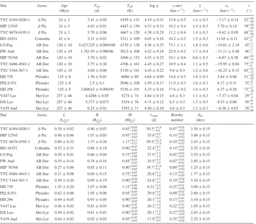
Table 2. Derived fundamental parameters for the stars in our sample.Protare the adopted rotation periods, containing a mix of literature and our

spectropo-larimetric periods, as discussed in Appendix A. Radial velocities (vr) are the averages and standard deviations of our observations. Lithium abundances are in

the form log (NLi/NH)+12.

Star Assoc. Age Prot Teff logg vsini ξ vr i

(Myr) (d) (K) (km s−1₎ _{(km s}−1₎ _{(km s}−1₎ ₍◦₎

TYC 6349-0200-1 βPic 24±3 3.41±0.05 4359±131 4.19±0.31 15.8±0.5 1.4±0.3 −7.17±0.14 52+20

−20

HIP 12545 βPic 24±3 4.83_±0.01 4447_±130 4.33_±0.23 10.2_±0.4 1.4_±0.3 7.70_±0.14 39+20

−20

TYC 6878-0195-1 βPic 24±3 5.70±0.06 4667±120 4.38±0.29 11.2±0.4 1.4±0.3 −8.62±0.09 68+22

−20

BD-16351 Columba 42±6 3.21±0.01 5211±109 4.65±0.16 10.2±0.3 1.5±0.3 11.05±0.11 42+17

−9

LO Peg AB Dor 120±10 0.423 229±0.000 048 4739±138 4.36±0.25 73.1±1.1 1.8±0.6 −19.81±2.18 45+3

−3

PW And AB Dor 120±10 1.761 59±0.000 06 5012±108 4.42±0.18 22.9±0.2 1.7±0.4 −11.11±0.48 46+7

−7

HIP 76768 AB Dor 120±10 3.70±0.02 4506±153 4.53±0.25 10.1±0.6 0.6±0.3 −6.87±0.38 60+30

−13

TYC 0486-4943-1 AB Dor 120±10 3.75±0.30 4706±161 4.45±0.27 10.9±0.4 1.1±0.5 −19.95±0.04 75+15

−8

TYC 5164-567-1 AB Dor 120±10 4.68±0.06 5130±161 4.45±0.22 9.6±0.3 1.2±0.6 −16.25±0.15 65+25

−12

HII 739 Pleiades 125±8 1.58±0.01 6066±89 4.64±0.09 14.8±0.3 1.8±0.3 5.64±0.08 51+20

−20

PELS 031 Pleiades 125±8 2.5±0.1 5046±108 4.59±0.17 11.9±0.3 1.6±0.3 6.17±0.31 35+8

−7

HII 296 Pleiades 125±8 2.608 63±0.000 09 5236±101 4.33±0.16 17.6±0.2 1.6±0.3 6.37±0.20 73+17

−20

V447 Lac Her-Lyr 257±46 4.4266±0.05 5274±74 4.64±0.15 4.6±0.3 1.1±0.3 −7.37±0.04 29+5

−4

DX Leo Her-Lyr 257±46 5.377±0.073 5354±76 4.71±0.12 6.5±0.3 1.3±0.3 8.53±0.08 58+8

−6

V439 And Her-Lyr 257±46 6.23±0.01 5393±71 4.50±0.10 4.6±0.3 1.3±0.3 −6.38±0.03 38+4

−4

Star Assoc. L R M τconv Rossby ALi

(L_⊙) (R_⊙) (M_⊙) (d) number (dex)

TYC 6349-0200-1 βPic 0.30±0.02 0.96±0.07 0.85+₋0₀._.05₀₅ 50.5+₋₆14_.₆.4 0.07₋+0₀._.01₀₂ 3.30±0.15 HIP 12545 βPic 0.40±0.06 1.07±0.05 0.95+₋0₀._.05₀₅ 55.8+₋₆6._.8₃ 0.14₋+0₀._.02₀₂ 3.40±0.15 TYC 6878-0195-1 βPic 0.80±0.32 1.37_±0.28 1.17+₋0₀._.13₂₁ 59.9+₋₁₇23._.5₈ 0.10₋+0₀._.04₀₃ 2.45±0.15 BD-16351 Columba 0.52_±0.21 0.88_±0.18 0.90₋+₀0._.07₀₅ 22.4₋+4₂._.₁5 0.14₋+₀0._.01₀₂ 2.25±0.15 LO Peg AB Dor 0.20±0.01 0.66±0.04 0.75+0.05

−0.05 27.9+−11..44 0.02+−00..0101 2.55±0.15

PW And AB Dor 0.35±0.14 0.78±0.16 0.85+0.05

−0.05 25.5+−42..65 0.07+−00..0101 2.85±0.15

HIP 76768 AB Dor 0.27±0.06 0.85±0.11 0.80+0.07

−0.05 39.7+−911.4.6 0.09+−00..0302 1.25±0.15

TYC 0486-4943-1 AB Dor 0.21±0.08 0.69±0.15 0.75+0.05

−0.05 28.8+−43..03 0.13+−00..0303 1.77±0.15

TYC 5164-567-1 AB Dor 0.50±0.20 0.89±0.19 0.90₋+₀0._.08₀₅ 24.8₋+74..15 0.19₋+00..0405 3.10±0.15

HII 739 Pleiades 1.35±0.20 1.07±0.06 1.15₋+00..0606 6.21−+20..36 0.25−+00..0108 3.00±0.15

PELS 031 Pleiades 0.62±0.06 1.05±0.06 0.95+0.05

−0.05 29.0+−53..84 0.09+−00..0202 2.80±0.15

HII 296 Pleiades 0.49±0.05 0.93±0.05 0.90₋+₀0._.05₀₅ 20.1₋+1₁..00 0.13−+00..0101 3.10±0.15

V447 Lac Her-Lyr 0.46±0.02 0.81±0.03 0.90₋+₀0._.05₀₅ 20.2₋+1₁._.₀0 0.22₋+₀0._.01₀₁ 1.95±0.15 DX Leo Her-Lyr 0.49_±0.02 0.81_±0.03 0.90₋+₀0._.05₀₅ 20.1₋+1₁._.₀0 0.27₋+₀0._.02₀₂ 2.65±0.15 V439 And Her-Lyr 0.64±0.02 0.92±0.03 0.95+0.05

−0.05 17.9+−00..99 0.35+−00..0202 2.25±0.15

is provided in Fig.1, and the final best parameters are reported in Table2.

In the computation of synthetic spectra we assumed solar abun-dances, from Asplund et al. (2009). We checked this assumption for a few stars (HII 739, TYC 6349-0200-1, and TYC 6878-0195-1) by performing a full abundance analysis simultaneously with the de-termination of the other stellar parameters. Solar abundances were consistently found, thus we conclude that this is a sufficiently good approximation for our analysis.

3.1.2 Secondary analysis

For all stars in the sample, we performed a secondary spectral analysis, using spectral synthesis from the 1D hydrostatic MARCS models of stellar atmospheres (Gustafsson et al.2008). This analysis produced lithium abundances (ALi), in addition toTeff, logg,vsini, and microturbulence values. We used a grid of plane–parallel model

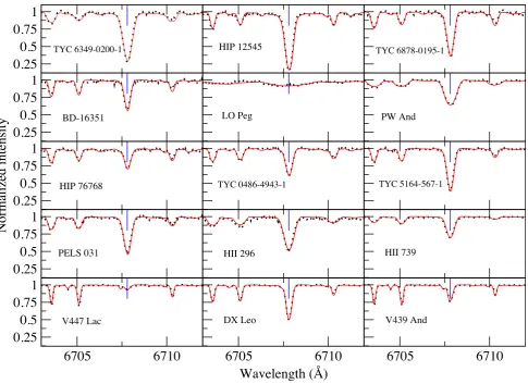
atmospheres in LTE, with solar abundances. The grid has steps of 250 K inTeffand steps of 0.5 dex in logg(note that specific abun-dances as well as metallicity – [Fe/H] – can be adjusted precisely through the spectral synthesis). To produce the high-resolution syn-thetic spectra of the lithium line region (at 6707.8 Å), we used the TURBOSPECTRUMcode (Alvarez & Plez1998) and an interpolation routine for MARCS model structures kindly provided by Masseron (private communication). Finally, we convolved the computed syn-thetic spectra with a Gaussian profile (in order to reproduce the instrumental profiles of ESPaDOnS and Narval), and by a rota-tional profile (to account for rotarota-tional velocity). Details of the complete method and of the detailed atomic and molecular line lists (initially extracted from the VALD data base) can be found in Canto Martins et al. (2011). Fits to the Li lines are presented in Fig.2.

This MARCS spectral synthesis analysis was done independently from the previously described analysis (ZEEMANspectral synthesis

(5)

[image:5.595.123.467.55.314.2]

Figure 1. Sample fit of the synthetic spectrum (red line) to the observation (black points) for HIP 12545.

Figure 2. Lithium line fits for the stars in this study, obtained with MARCS spectral synthesis. Observations are dotted lines, the fits are solid lines and the Li line position is indicated by a thin vertical (blue) line.

[image:5.595.54.540.341.694.2]

(6)

analysis). It then provided a crosscheck for all the stellar parameters produced through theZEEMANspectral synthesis. IndeedTeff, logg, [Fe/H],vsini, and microturbulence velocity have also been deter-mined using MARCS synthetic spectra (mainly from the lithium line region, with checks from regions around the Ca infrared – IR – triplet and Hβ). The stellar parameters derived from MARCS spectral synthesis have been used for the ALi determination. A conservative accuracy of 0.15 dex has been adopted for theALi determinations, considering an accuracy of 50 K onTeff; 0.5 dex on logg; 0.15 dex on [Fe/H]; 0.5 km s−1_on_v_sin_i_{; 0.5 km s}−1_on microturbulence velocity.

3.1.3 Spectroscopic comparison

In general, a good agreement for all the stellar parameters was found between the two approaches (ZEEMANversus MARCS spec-tral synthesis). Some specific cases, however, present discrepan-cies on some parameters. Ourvsini, measurements are consistent within 1σ for all stars except LO Peg, where we disagree at 1.9σ (73.1±1.1 and 67±3 km s−1_{). The}_v_sin_i_{, value of Barnes et al.} (2005, 65.84±0.06 km s−1_{) is smaller than both our values, but} consistent with the MARCS value. LO Peg has the broadest line profiles, and the line profiles most affected by spots. Thus it is not surprising that our methods disagree slightly, due to the distorted line profiles. Our measurements of microturbulence agree typically within 1σ, and always within 1.5σ. Our loggmeasurements always agree within 1σ. This suggests we may have overestimated the un-certainties on logg; however, in the interest of caution we retain the current values. OurTeffvalues generally agree within 1σ; however, there are a few significant disagreements. Our results disagree at 3σ (∼300 K: 6066±89 and 5750±50 K) for HII 739. This star is a spectroscopic binary, with a small radial velocity separation, and the lines of the two components largely superimposed. Since the analyses use different selections of lines in different wavelength windows this produces different results. We adopt the hotterTeff, obtained from the bluer part of the spectrum, as this is likely less in-fluenced by contamination from the secondary. There is a significant disagreement in ourTefffor LO Peg, by 3.5σ (500 K: 4739±138 and 5250_±50 K). This is likely due to the large distortions to the line profiles by star spots, and blending of lines due to the large vsini. We adopt the value based on the larger number of spectral lines, which should mitigate the impact of line profile distortions, and this value is consistent with the literature values (Jeffries et al. 1994; Bailer-Jones2011; McCarthy & White2012). However, this difference may represent a real uncertainty on theTeffof LO Peg, due to its large spots. For BD-16351 theTeffmeasurements differ by 1.8σ (210 K: 5211±109 and 5000±50 K); however, there is no clear error with either value. da Silva et al. (2009) find a

Teffof 5083 K for BD-16351, approximately halfway between our values. OurTeffmeasurements for HII 296 differ by 2.1σ (236 K: 5236±101 and 5000±50 K), again with no clear errors in either value. Several literatureTeffmeasurements exist for HII 296, which fall in the range 5100–5200 (Cayrel de Strobel1990; Cenarro et al. 2007; Soubiran et al.2010; Prugniel, Vauglin & Koleva2011), thus between our two values but favouring the higher value. The formal disagreements inTefffor BD-16351 and HII 296 are acceptable, and are likely a reflection of the real systematic uncertainties involved. Ultimately we adopt theTeffvalues from theZEEMANanalysis, in order to provide a homogeneous set of values, since the values are largely consistent, and of comparable quality.

3.2 H–R diagram and evolutionary tracks

3.2.1 H–R diagram positions

Absolute luminosities for the stars in this sample were derived from

J-band photometry, from the 2MASS project (Cutri et al.2003). IR photometry is preferable to optical photometry since it is likely impacted less by star spots. This is because the brightness contrast between spots and the quiescent photosphere is less in the IR. The stars are all nearby, so interstellar extinction is likely negligible. However, IR photometry further mitigates any possible impact of extinction. Finally, 2MASS provides a homogeneous catalogue of data for the stars in our study. The bolometric correction from Pecaut & Mamajek (2013) was used combined with our effective tempera-tures (from Section 3.1). Pecaut & Mamajek (2013) include results for the 2MASSJband, and for PMS stars. We assume reddening is negligible, since the stars are all near the Sun (<130 pc). From this we calculate the absolute luminosities, presented in Table2.

Six stars have precise, reliableHipparcosparallax measurements. We use the re-reduction of theHipparcos data by van Leeuwen (2007). The star TYC 6349-0200-1 does not have aHipparcos mea-surement, but it has a physical association with HD 199143 (van den Ancker et al.2000), which was observed byHipparcos. There-fore we use the parallax of HD 199143 for TYC 6349-0200-1 (e.g. Evans et al.2012). For the Pleiades, there has been a longstanding disagreement regarding the distance, particularly between the Hip-parcosparallax of van Leeuwen (2009) and theHSTtrigonometric parallax of Soderblom et al. (2005). The recent VLBI parallax of Melis et al. (2014) strongly supports theHSTvalue, thus we adopt their value and take the uncertainties on stellar distances as their estimate of the dispersion in cluster depth. The difference between these distances is∼10 per cent, and this degree of uncertainty has no major impact on our results. For the other stars we use the dy-namical distances, mostly from Torres et al. (2008), supplemented by Montes et al. (2001) and Torres et al. (2006). These dynamical distances are based on the proper motion of a star, and are the dis-tance to the star that makes its real space velocity closest to that of its association’s velocity. For these dynamical distances we adopt a 20 per cent uncertainty, which is a conservative assumption since the authors do not provide uncertainties. The adopted distances are included in Table3.

With absolute luminosities and effective temperatures, we can infer stellar radii from the Stefan–Boltzmann law. We can also use this information to place the stars on an H–R diagram, shown in Fig.3. By comparison with theoretical evolutionary tracks we can estimate the masses of the stars.

3.2.2 Evolutionary models

We used a grid of evolutionary tracks to be published in Amard et al. (in preparation). Standard stellar evolution models with masses from 0.5 to 2 M_⊙were computed with theSTAREVOLV3.30 stellar evolu-tion code. The adopted metallicity isZ=0.0134, which corresponds to the solar value when using the Asplund et al. (2009) reference so-lar abundances. The adopted mixing length parameterαMLT=1.702 is obtained by calibration of a classical (without microscopic dif-fusion) solar model that reproduces the solar luminosity and radius to 10−5_{precision at 4.57 Gyr. The models include a non-grey} at-mosphere treatment following Krishna Swamy (1966). Mass-loss is accounted for starting at the ZAMS following Reimers (1975). The convective boundaries are fixed by the Schwarzschild criterion, and the local convective velocities are given by the mixing length theory.

(7)

[image:7.595.133.457.71.256.2]

Table 3. Literature fundamental parameters for the stars in our sample.

Star Assoc. Age Distance Distance

(Myr) (pc) method

TYC 6349-0200-1 βPic 24±31 _45.7_±_1.62, 3 _{Assoc. Parallax}

HIP 12545 βPic 24±31 _42.0_±_2.72 _Parallax

TYC 6878-0195-1 βPic 24±31 ₇₉_±₁₆4 _Dynamical

BD-16351 Columba 42±61 ₇₈_±₁₆5 _Dynamical

LO Peg AB Dor 120±106 _40.3_±_1.12 _Parallax

PW And AB Dor 120±106 _30.6_±_6.17 _Dynamical

HIP 76768 AB Dor 120_±106 _40.2_±_4.42 _Parallax

TYC 0486-4943-1 AB Dor 120±106 ₇₁_±₁₄5 _Dynamical

TYC 5164-567-1 AB Dor 120±106 ₇₀_±₁₄5 _Dynamical

HII 739 Pleiades 125±88 _136.2_±_2.39 _{Assoc. Parallax}

PELS 031 Pleiades 125±88 _136.2_±_2.39 _{Assoc. Parallax}

HII 296 Pleiades 125±88 _136.2_±_2.39 _{Assoc. Parallax}

V447 Lac Her-Lyr 257_±4610 _46.4_±_0.52 _Parallax

DX Leo Her-Lyr 257_±4610 _56.2_±_0.62 _Parallax

V439 And Her-Lyr 257_±4610 _73.2_±_0.62 _Parallax

Age references:1_{Bell, Mamajek & Naylor (}₂₀₁₅_),6_{Luhman, Stauffer & Mamajek (}₂₀₀₅_{) and Barenfeld}

et al. (2013),8_{Stauffer, Schultz & Kirkpatrick (}₁₉₉₈_),10_{L´opez-Santiago et al. (}₂₀₀₆_{) and Eisenbeiss}

et al. (2013). Distance references:2_{van Leeuwen (}₂₀₀₇_),3_{van den Ancker et al. (}₂₀₀₀_),4_{Torres et al.}

[image:7.595.45.281.324.499.2]

(2006),5_{Torres et al. (}₂₀₀₈_),7_{Montes et al. (}₂₀₀₁_),9_{Melis et al. (}₂₀₁₄_).

Figure 3. H–R diagram for the stars in this study. Evolutionary tracks (solid lines) are from Amard et al. (in preparation), and are shown for 0.1 M_⊙ increments from 0.5 to 1.5 M_⊙. Isochrones are shown for 24 Myr (βPic), 42 Myr (Columba), and the ZAMS. Stars grouped by association and age, as indicated.

This allows us to compute the convective turnover time-scale at one pressure scaleheight above the base of the convective envelope, for each timestep:

τHp=αHp(r)/Vc(r), (1)

whereVc(r) is the local convective velocity as given by the mixing length theory formalism at one pressure scaleheight above the base of the convective envelope,Hp(r) is the local pressure scaleheight, and αis the mixing length parameter. This choice of convective turnover time-scale is discussed in Appendix D.

In order to derive an estimate of the masses and convective turnover time-scales (and hence Rossby numbers) for the stars in our sample, we use the maximum-likelihood method described in

Figure 4. Longitudinal magnetic field measurements for TYC 6349-200-1, phased with the rotation periods derived in Section 4.3. The solid line is the fit through the observations. Figures for the full sample can be found in Appendix A.

Valle et al. (2014). We based our estimates uponTeffand luminosity, and the associated error bars derived from our analysis.

3.2.3 Comparison to association isochrones

From these model evolutionary tracks we computed isochrones for the age of each association. Comparing the observed stars positions on the H–R diagram with the model association isochrones, we find that the H–R diagram positions are consistent with the adopted ages for most stars. This supports the association memberships of those stars. However a few stars disagree with their isochrones by more than 2σ, suggesting unrecognized systematic errors, or underestimated uncertainties. HII 739 appears to sit well above the association isochrone (at the ZAMS for thatTeff), but it is a binary. HIP 12545 sits somewhat below the association isochrone

[image:7.595.308.542.325.502.2]

(8)

by slightly more than 2σ, possibly suffering some extinction, but still is well above the ZAMS. HIP 76768 sits marginally above its isochrone (at the ZAMS), but by less than 2σ. PELS 031 also sits above its isochrone, by 2σ; however, there is no clear evidence that it is a spectroscopic binary. These discrepancies are not due to metallicity, since the members of one association should have the same metallicity, and there is no observational evidence for significantly non-solar metallicities in our sample. For the most discrepant cases, HII 739 and HIP 12545, we derive the stellar parameters usingTeffand the age of their association, rather than luminosity. For these two stars we also adopt the radii from the evolutionary tracks rather than Stefan–Boltzmann law.

We use the masses derived from the H–R diagram and the stel-lar radii to calculate a logg for the stars. Comparing this with the spectroscopic loggwe derived earlier shows that the values are consistent. For the binary HII 739, this is only true if we use values based onTeffand age, rather than luminosity. Many of the loggvalues from evolutionary radii and masses are formally more precise than the spectroscopic values; however, we prefer the spec-troscopic values for this study as they have fewer potential sources of systematic uncertainty.

4 S P E C T RO P O L A R I M E T R I C A NA LY S I S

4.1 Longitudinal magnetic field measurements

Measurements of the longitudinal component of the magnetic field, averaged across the stellar disc, were made from all the individual LSD profiles. This provides much less information than a full ZDI map, but it depends much less on other stellar parameters (e.g. rota-tion period, inclinarota-tion,vsini). The longitudinal magnetic field was measured using the first-order moment method (e.g. Rees & Semel 1979), by integrating the (continuum normalized) LSD profilesI/Ic andV/Icabout their centre-of-gravity (v0) in velocity (v):

Bℓ=−2.14×1011

!

(v−v0)V(v) dv

λgfc !

[1−I(v)] dv

. (2)

Here the longitudinal fieldBℓis in Gauss,cis the speed of light, and

λ(the central wavelength, expressed in nm) andgf(the Land´e factor) correspond to the normalization values used to compute the LSD profiles (see Section 2.2). The integration range used to evaluate the equation was set to include the complete range of the absorption line inI, as well as inV. The resulting measurements ofBℓ are

summarized in Table4and plotted, folded with the stellar rotation periods (see Section 4.3), in Fig.4as well as FigsA2andA3.

The longitudinal magnetic fields, which vary due to rotational modulation, were used to determine a rotation period for each star. This was done by generating periodograms, using a modified Lomb– Scargle method, for each star. The periodograms were generated by fitting sinusoids through the data using a grid of periods, thus producing periodograms in period andχ2. The sinusoids were in the form

n "

l=0

alsinl(p+φ), (3)

wherenis the order of the sinusoid used,alandφare free parame-ters, andpis the period for each point on the grid. This formalism has the advantage of easily accounting for magnetic fields with significant quadrupolar or octupolar components, and reduces to

a Lomb–Scargle periodogram whenn=1. Searches for a period Ta

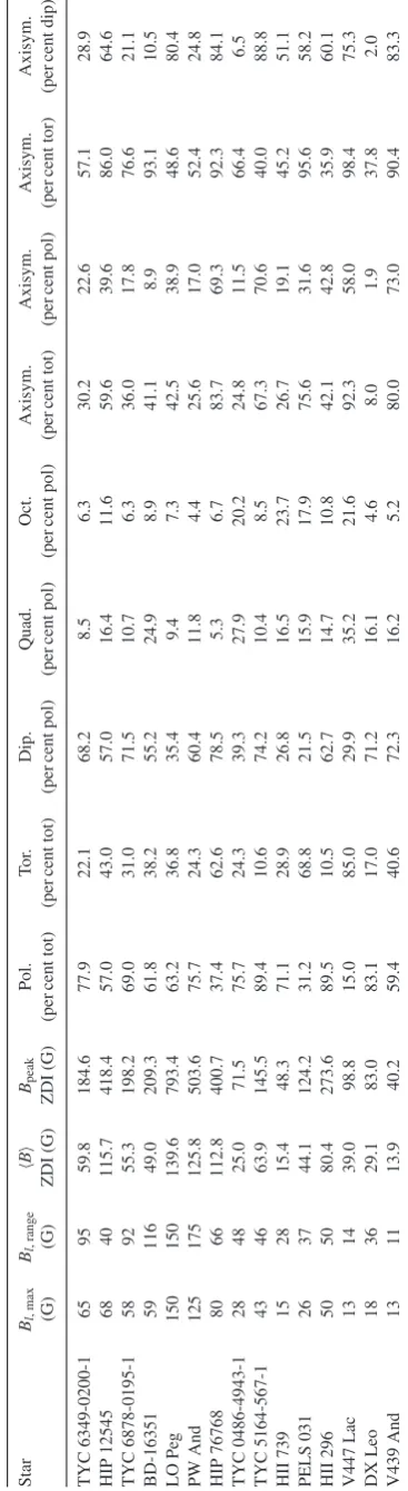
bl e 4. Deri ve d m agnetic properties for the stars in our sample. The m aximum disc inte grated longitudinal m agnetic field is in column 2, and the amplitude of va riability in the longitudinal field is in column 3. The surf ace-a veraged lar ge-scale magnetic field strength from the ZDI m ap is in column 4, and the maximum field value from the ZDI m ap is in column 5. The remaining columns present the percent of the magnetic ener gy in dif ferent components of the field. Star

Bl,m

ax

Bl,r

ange ⟨ B ⟩ Bpeak Pol. To r. Dip. Quad. O ct. Axisym. A xisym. Axisym. A xisym. (G) (G) ZDI (G) ZDI (G) (per cent tot) (per cent tot) (per cent pol) (per cent pol) (per cent pol) (per cent tot) (per cent pol) (per cent tor) (per cent dip) TYC 6349-0200-1 65 95 59.8 184.6 77.9 22.1 68.2 8.5 6.3 30.2 22.6 57.1 28.9 HIP 12545 68 40 115.7 418.4 57.0 43.0 57.0 16.4 11.6 59.6 39.6 86.0 64.6 TYC 6878-0195-1 58 92 55.3 198.2 69.0 31.0 71.5 10.7 6.3 36.0 17.8 76.6 21.1 BD-16351 59 116 49.0 209.3 61.8 38.2 55.2 24.9 8.9 41.1 8.9 93.1 10.5 LO Pe g 150 150 139.6 793.4 63.2 36.8 35.4 9.4 7.3 42.5 38.9 48.6 80.4 PW And 125 175 125.8 503.6 75.7 24.3 60.4 11.8 4.4 25.6 17.0 52.4 24.8 HIP 76768 80 66 112.8 400.7 37.4 62.6 78.5 5.3 6.7 83.7 69.3 92.3 84.1 TYC 0486-4943-1 28 48 25.0 71.5 75.7 24.3 39.3 27.9 20.2 24.8 11.5 66.4 6.5 TYC 5164-567-1 43 46 63.9 145.5 89.4 10.6 74.2 10.4 8.5 67.3 70.6 40.0 88.8 HII 739 15 28 15.4 48.3 71.1 28.9 26.8 16.5 23.7 26.7 19.1 45.2 51.1 PELS 031 26 37 44.1 124.2 31.2 68.8 21.5 15.9 17.9 75.6 31.6 95.6 58.2 HII 296 50 50 80.4 273.6 89.5 10.5 62.7 14.7 10.8 42.1 42.8 35.9 60.1 V447 Lac 13 14 39.0 98.8 15.0 85.0 29.9 35.2 21.6 92.3 58.0 98.4 75.3 DX Leo 18 36 29.1 83.0 83.1 17.0 71.2 16.1 4.6 8.0 1.9 37.8 2.0 V439 And 13 11 13.9 40.2 59.4 40.6 72.3 16.2 5.2 80.0 73.0 90.4 83.3

[image:8.595.350.534.60.731.2]

(9)

began withn=1, and if no adequate fit to the observations could be obtained, the order was increased to a maximum ofn₌3.

These results usually produced well-defined minimum in χ2, often with harmonics at shorter periods. However the results for five stars were ambiguous (HIP 12545, PELS 031, HII 296, HII 739, and V447 Lac), with comparableχ2minima at multiple periods. For stars with a well-defined minimum, we can use the change in χ2 from that minimum to provide uncertainties on the period (e.g. Press et al.1992). The periods found here typically have less precision than the literature photometric period estimates. This is a consequence of the relatively short time-span over which the observations were collected (typically one to two weeks).

For three stars, our adopted period (see Section 4.3 and Ap-pendix A) produced a particularly poor phasing of theBℓ curves.

For LO Peg, the rotation period is well established both by Barnes et al. (2005) and by our ZDI results. While there is a lot of apparent scatter in theBℓcurve, the first-order fit producesχν2=1.1. TheBℓ

curve of HIP 12545 appears, by eye, to indicate a harmonic of the true period. However examining the phasing of LSD profiles shows a consistent phasing at this period and inconsistent phasings at the possible alternatives; thus, this must be the correct period. For HII 739, there is very little variation in the longitudinal field curve, with the exception of two observations obtained 10 d earlier than the rest of the data. There is much clearer variability in the LSDVprofiles, and modelling those is what the period was principally based on; however, noise is a limiting factor in our analysis of this star.

We find a wide range of longitudinal magnetic fields. The strongest star reaches a Bℓ of 150 G, most stars at most phases

haveBℓof a few tens of gauss, and a few stars haveBℓbelow 10 G

at many phases, as summarized in Table4. We consider the maxi-mum observedBℓas a proxy for the stellar magnetic field strength,

to mitigating geometric effects and rotational variability (similar to, e.g. Marsden et al. 2014). In the maximumBℓ, two stars

ex-ceed 100 G, four stars are below 20 G, and the median is_∼50 G. There is an approximate trend of weakening maximumBℓwith age,

the youngest (_∼20 Myr) stars have stronger fields than the oldest (∼257 Myr); however, there is a very large scatter for the interme-diate age stars (∼120 Myr). There is also a weak trend in rotation rate, with the fastest rotating stars having the strongest fields. A clearer correlation in decreasingBℓwith Rossby number is found.

More detailed magnetic results, accounting for magnetic and stellar geometry, are presented in Section 5.

4.2 Radial velocity

Radial velocities for each observation were measured from the LSD profiles. These values were measured by fitting a Gaussian line pro-file to the StokesILSD profile, which effectively uses the Gaussian fit to find the centroid of the profile. The radial velocity variability observed is not a real variation in the velocity of the star (with the partial exception of close binaries), but rather due to distortions in the line profile from spots on the stellar surface. These distortions are modulated with the rotation period of the star, and thus the ap-parent radial velocity variation can be used to measure the rotation period of the star.

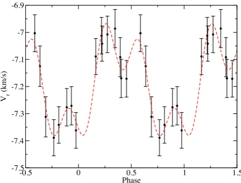
The same modified Lomb–Scargle analysis method that was used to derive a period from the longitudinal field measurements was applied to the radial velocity measurements. See Fig.5for an ex-ample. The surface spot distribution is generally more complex than the large-scale magnetic field distribution, and consequently the re-sults of this analysis were more ambiguous than they were for the magnetic field analysis. Six stars displayed periodograms with

mul-Figure 5. Radial velocity measurements for TYC 6349-200-1, phased with the rotation period derived in Section 4.3. The dashed line is a second-order sine fit through the observations.

tiple ambiguousχ2minima (HIP 12545, BD-16351, PELS 031, HII 296, HII 739, and V447 Lac). However, the periods found from the magnetic analysis were always consistent with one of the stronger minima from radial velocity. Thus the apparent radial velocity vari-ability supports periods based on the longitudinal magnetic fields, but is not always sufficient to determine a period on its own.

The observation that radial velocity variability is more ambiguous and less sensitive to rotation periods than magnetic variability has important implications for surveys aimed at characterizing planets around active stars. This implies that spectropolarimetric observa-tions are much more useful for characterizing the stellar part of the variability than simple spectroscopic observations.

4.3 Rotation period

All of the stars in our sample have literature rotation periods. How-ever, there is the potential for large systematic errors in these periods. For example, nearly identical spot distributions on either side of a star can cause a period to be underestimated by a factor of 2. Indeed a few of the stars in our sample have conflicting literature periods. Having an accurate rotation period is critical for an accurate ZDI map so we verified and, when possible, rederived rotation periods for all the stars in the sample.

Our period search used three methods. The first technique was based on longitudinal magnetic field measurements, and is de-scribed in Section 4.1. This method has the advantage of being largely model independent; however, the method loses sensitivity for more complex magnetic geometries and for largely toroidal magnetic geometries. The second method was based on apparent radial velocity variability, as a measure of line profile variability due to spots (cf. Section 4.2). Most of the stars are only weakly spotted, and thus in many cases this variability is only weakly detected. Fur-thermore the variability in apparent radial velocity is usually more complex than the variability in the longitudinal magnetic field. Thus the radial velocity variability was only used to confirm the rotation period measurements from the other two methods. The third method was based on the ZDI analysis, searching for a period that produced the maximum entropy ZDI map (e.g. Petit et al.2008). Details of the ZDI procedure are given in Section 5. Since we use the fitting routine of Skilling & Bryan (1984), entropy rather thanχ2is the correct parameter to optimize. This rotation period search starts

[image:9.595.306.544.56.236.2]

(10)

with a grid of rotation periods, and for each period recomputes the phases of the observations, then runs ZDI. From this we produce a plot of entropy as a function of rotation period, and select the period that maximizes entropy. This method of period searching is more model dependent than the method based on longitudinal magnetic fields. However, this method is more sensitive when the magnetic field geometry is complex, since it consistently models all the information available in the StokesVprofiles.

In most cases, all the period estimates agree with the literature values. In a few cases, TYC 0486-4943-1, HII 739, and PELS 031, the literature periods were inconsistent with our observations. The final rotation periods we adopt are in Table2. Detailed discussions of our analyses and comparisons with literature values for all the stars are given in Appendix A.

Emission indices were calculated for the CaIIH&K lines, Hα, and the Ca IR triplet, summarized in Appendix C. These quantities usually vary coherently with rotation phase, but do not do so in a simple fashion, and thus were not used for period determination.

Values for the inclination of the rotation axis with respect to the line of sight were derived using two methods. When possible, the value was based onvsiniand the combination of radius and period to determine an equatorial velocity (veq). However, in a few cases the radius was poorly constrained, either due to an uncertain mag-nitude in a binary system, or due to an uncertain distance to the star. In these cases a second method was used, looking for the inclination that maximizes entropy in ZDI. This was done in the same fashion as the ZDI period search, searching a grid of inclinations and se-lecting the one with the maximum entropy ZDI solution. This ZDI based inclination was checked against the inclination fromvsini, radius and period, for cases with well-defined radii, and a good agreement was consistently found. The adopted best inclinations are given in Table2, and in cases where the ZDI inclination was used, a discussion of the inclination determination is provided in Appendix A.

5 M AG N E T I C M A P P I N G

5.1 ZDI model description

ZDI was used to reconstruct surface magnetic field maps for all the stars in this study. ZDI uses the observed rotationally modulated StokesVline profiles, and inverts the time series of observations to derive the magnetic field necessary to generate them. We used the ZDI method of Semel (1989), Donati & Brown (1997), and Donati et al. (2006), which represents the magnetic field as a combination of spherical harmonics, and uses the maximum entropy regular-ization procedure described by Skilling & Bryan (1984). ZDI was performed using the StokesVLSD profiles, which was necessary to provide sufficiently large S/N.

ZDI proceeds by iteratively fitting a synthetic line profile to the observations, subject to bothχ2and the additional constraint pro-vided by regularization, using the spherical harmonic coefficients that describe the magnetic field as the free parameters. Therefore the model line profile used is of some importance. We calculated the local StokesVline profile, at one point on the stellar surface, using the weak field approximation:

V(λ)=−λ2_o gfe 4πmec

BldI /dλ, (4)

whereλois the central wavelength of the line,gfis the mean Land´e factor, andBlis the line of sight component of the magnetic field.

The local Stokes I profile is approximated as a continuum level minus a Gaussian. The local line profiles are then weighted by the projected area and brightness of their surface element, calculated using a classical limb darkening law, and Doppler shifted by their rotational velocity. The local profiles are summed, and finally nor-malized by the sum of their continuum levels and projected cell areas to produce a final disc integrated line profile. In this study we have assumed surface brightness variations due to star spots are negligible. While these brightness variations are detectable in some StokesIprofiles, they are small (1–5 per cent of the line depth), and the impact of this variability would be lost in the noise of the observed StokesVprofiles (Vprofiles are typically observed with

∼5σ precision per pixel).

Since we are modelling LSD profiles, the mean Land´e factor and central wavelength used for the model line were set to the normal-ization values used for LSD (Kochukhov et al.2010). The width of the Gaussian line profile was set empirically by fitting the line width of the very slow rotatorϵ Eri (Jeffers et al.2014), which has a spectral type typical of the stars in our sample (K2). LSD was applied to the spectrum of ϵ Eri with the same normaliza-tion and line masks as used for the rest of the stars in this study. The ZDI modelIline profile was then fit to the LSDIline profile of the star, providing a Gaussian line width. We also checked the line width used against theoretical models. A synthetic line profile was calculated using theZEEMANspectrum synthesis program for a star withTeff=5000 K, logg=4.5, and 1.2 km s−1of micro-turbulence, approximately average for the stars in this study, but no rotation. The atomic data for this model line were taken to be the average of the atomic data used for the lines in the LSD line mask. Line broadening included the quadratic Stark, radiative, and van der Walls effects, as well as thermal Doppler broadening. This detailed synthetic line profile was then fit with the Gaussian ZDI line model, to find a theoretical best width for the ZDI line profile. Good agreement was found, with the theoretical width and the em-pirical width fromϵEri differing by less than 10 per cent; thus, a full width at half-maximum of 7.8 km s−1_(1σ _{width of 3.2 km s}−1₎ was adopted for the ZDI model line. Line depths were set individ-ually for each star in the study, by fitting the central depth of the ZDI StokesIline to the central depth of the average LSDI line profile.

For the stellar model we used in ZDI,vsiniwas taken from the spectroscopic analysis in Section 3.1. A linear limb darkening law was used with a limb darkening coefficient of 0.75, typical of a K star at our model line wavelength (Gray2005). The ZDI maps are largely insensitive to the exact value of the limb darkening parameter (e.g. Petit et al.2008). The inclination of the stellar rotation axis to the line of sight was determined from stellar radius andvsini from Section 3 and the rotation period used for the star was derived in Section 3. Differential rotation was assumed to be negligible; however, this will be investigated further in the next paper in this series. The exception to this is LO Peg, where a reliable literature differential rotation measurement exists.

The model star was calculated using 2000 surface elements of approximately equal area, and the spherical harmonic expansion was carried out to the 15th order inl. For our spectral resolution and local line with, and a typicalvsiniof 10 km s−1, Morin et al. (2010) suggest that only the first_∼8 harmonics should carry any useful information (at avsiniof 15 km s−1that becomes the first 10 harmonics). This matches our results, as in all cases the magnetic energy in the coefficients drops rapidly by fifth order, often sooner, with the coefficients being driven to zero by the maximum entropy regularization.

(11)

[image:11.595.48.285.50.557.2]

Figure 6. Sample ZDI fit for TYC 6349-200-1. The solid lines are the observed LSDV/Icprofile and the dashed lines are the fits. The profiles are

shifted vertically according to phase and labelled by rotation cycle. 5.2 ZDI results

A sample ZDI fit is presented in Fig.6. The resulting magnetic maps are presented in FigsA4andA5. Several parameters describing the magnetic strength and geometry are given in Table4. The mean magnetic field (⟨B⟩) is the global average strength of the (unsigned) large-scale magnetic field over the surface of the star (i.e. the mag-nitude of the magnetic vector averaged over the surface of the star). The field is broken into poloidal and toroidal components (as in Donati et al.2006), into axisymmetric (m=0 spherical harmonics) and non-axisymmetric components, and the fraction of the mag-netic energy (proportional toB2_{) in different components is given.}

Note that in some cases, the values are considered as fractions of the total magnetic energy, and in some cases they are fractions of one component, such as the fraction of poloidal energy in the dipolar mode.

We find a wide range of magnetic strengths and geometries. Mean magnetic field strengths vary from 14 to 140 G, with some dependence on age and rotation rate. The magnetic field geometries vary from largely poloidal to largely toroidal. The majority (12/15) of the stars have the majority of their magnetic energy in poloidal modes; however, there are significant toroidal components found in many stars. There is a large range of observed axisymmetry, and the majority of the stars have the majority of their energy in non-axisymmetric components. There is also a wide range of complexity (dominantlorder) to the fields. However, none of the observed stars are entirely dipolar or entirely axisymmetric. This diversity of magnetic properties is qualitatively typical of stars with radiative cores and convective envelopes (e.g. Donati & Landstreet 2009).

6 D I S C U S S I O N

This discussion focuses on the large-scale magnetic properties of our sample, and trends in those properties with the physical parameters of age, rotation period, mass, and Rossby number. We then compare our results to those for younger TTS and older field stars, in order to provide a synthetic description of the magnetic evolution of solar-type stars from the early PMS to the end of the MS.

6.1 Magnetic trends in young stars

6.1.1 Trends in magnetic strength

Several trends are apparent from our sample, that are illustrated in Fig.7. We find a global decrease in the mean large-scale magnetic field strength with age from 20 to 250 Myr, even though a large scatter is seen at intermediate ages at around 120 Myr. 120 Myr is also the age with maximum scatter in rotation period. No clear trend between mean magnetic field strength and rotation period is seen in our limited sample. Similarly, we do not find any clear trend in magnetic field strength with just convective turnover time. However, conventional (α–-) dynamo generation is thought to be due to the combination of rotation and convection, which can be parametrized by the Rossby number of the star (the ratio of the rotation period to the convective turnover time:Ro= Prot/τconv). We do find a significant trend in decreasing magnetic field strength with Rossby number, which appears to take the form of a power law. Fitting a power law (and excluding LO Peg, the fastest rotator) we find⟨B⟩ ∝R−1.0±0.1

o . This is based on aχ2fit, and accounts for uncertainty inRobut not the systematic uncertainty in⟨B⟩, which is largely driven by long term variability; thus, the uncertainty on the power law may be underestimated. LO Peg, the outlier, has by far the lowest Rossby number in our sample, but has a comparable field strength to the other strongly magnetic stars in our sample. This suggests that we might be seeing evidence for the saturation of the global magnetic field strength and hence of the stellar dynamo. Saturation of CaIIH&K emission (Noyes et al.1984), and X-ray flux (Pizzolato et al.2003), is well established and typically happens around a Rossby number of 0.1.2_{Zeeman broadening measurements}

2_{The exact value of the Rossby number is model dependent, since it depends}

on the prescription for convective turnover time. Thus it can vary by a factor of a few (see Appendix D).

(12)

[image:12.595.68.533.53.415.2]

Figure 7. Trends in global mean large-scale magnetic field strength with age, rotation period, and Rossby number for the stars in our sample. Different symbols correspond to different age bins.

(Saar1996,2001; Reiners et al.2009) have found some evidence for the saturation of the small-scale magnetic field, again around a Rossby number of 0.1, particularly for M-dwarfs. Evidence for saturation of the global magnetic field is good for fully convective M-dwarfs (Donati et al.2008b; Morin et al.2008; Vidotto et al. 2014). However, direct evidence for the saturation of the global magnetic field in stars with radiative cores remains tentative. Vidotto et al. (2014) studied a set of published ZDI results, which includes the data reported here, and found evidence for the global dynamo saturating near the same Rossby number as the X-ray flux. LO Peg adds a significant extra data point to support this trend. It is interesting that the X-ray flux, which is only indirectly related to the magnetic field, the small-scale magnetic field, and the large-scale magnetic field all show qualitatively similar behaviour with Rossby number.

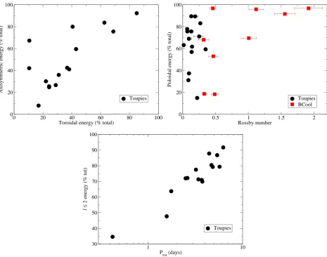
6.1.2 Trends in magnetic geometry

Turning to magnetic topology, we find that stars with largely toroidal magnetic fields in our sample have largely axisymmetric geome-tries, as shown in Fig.8. More specifically the toroidal components of the magnetic field are largely axisymmetric, and become more axisymmetric as they become more dominant. However, the axisym-metry of the poloidal component is independent of how toroidal the field is, thus the trend towards axisymmetry is driven by the toroidal

component. This is in line with similar results reported for a larger sample of late-type dwarfs by See et al. (2015), which also includes the results presented here. We also examined the fraction of mag-netic energy contained in the poloidal component as a function of rotation period, shown in Fig.8. No clear trend is seen in our sam-ple, which encompasses a limited range of rotation periods from about 2 to 6 d. Indeed, within this period range, the fraction of mag-netic energy contained in the poloidal component ranges from 15 to 90 per cent. In order to enlarge the period range, we combine our sample with the slowly rotating stars reported by Petit et al. (2008), and with additional slow rotators from the BCool sample (Petit et al., in preparation; see Section 6.2). Petit et al. (2008) re-ported that slowly rotating stars have dominantly poloidal fields and rapidly rotating stars have dominantly toroidal fields. The stars of our HMS sample all lie in the fast portion of their parameter space and exhibit a large range of poloidal to toroidal ratios. If we con-sider the additional data from the BCool project, we do indeed find that very slow rotators are dominated by poloidal fields, but faster rotators have a wide range of mixed geometries. The transition from mixed topologies to dominantly poloidal fields seems to occur at roughlyProt ≈10–15 d, in agreement with Petit et al. (2008). In Rossby number, this transition occurs roughly between 0.5 and 1.0 (cf. Fig.8).

We examined the complexity of the reconstructed large-scale magnetic field, by considering the magnetic energy in all spherical

(13)

[image:13.595.59.525.61.427.2]

Figure 8. Trends in magnetic geometry. Left panel: the fraction of magnetic energy in axisymmetric modes as a function of the fraction of magnetic energy in toroidal modes (our data only). Right panel: the fraction of magnetic energy in poloidal modes as a function of Rossby number (our data and BCool data). A shift towards dominantly poloidal fields, from mixed toroidal-poloidal fields, is found for stars with long rotation periods. Bottom panel: fraction of magnetic energy in spherical harmonics of orderl≤2, as a function of rotation period (our data only).

harmonic modes withl≤2. This includes dipolar and quadrupolar modes, and their corresponding toroidal modes. We find a trend towards decreasing complexity with increasing rotation period, il-lustrated in Fig.8, and a similar trend with increasing Rossby num-ber. Thus it may be that faster rotators, with stronger dynamos, have more complex magnetic fields. This is in contrast to the fully convective TTS that often have simple magnetic field geometries. However, the spatial resolution of ZDI is a function of thevsiniof a star; thus, there is a potential systematic effect that could impact on this result. The correlation we find appears to be stronger with rotation period thanvsini, and all our stars should have maps with a resolution higher than anlorder of 2, thus this trend appears to be real. Nevertheless, we caution the reader that this result is tenta-tive. A more detailed investigation, with an evaluation of potential systematics, is needed and planned for a forthcoming paper.

6.1.3 Implications for models

Barnes (2003) identified the C and I sequences of, respectively, fast and slow rotating young MS stars. In an attempt to reproduce these sequences, Brown (2014) proposed the ‘Metastable Dynamo

Model’ of rotational evolution. In this model, stars are initially very fast rotators and are weakly coupled to their winds. Eventually, stars

randomlyswitch to being strongly coupled to their wind, and then quickly spin down. The difference between the weakly and strongly coupled modes is ascribed to different magnetic topologies, hy-pothetically corresponding to different dynamo modes. However, within our sample we find no strong differences in magnetic geom-etry between very fast rotators (Prot <2 d) and moderate rotators (Prot>2 d), which would essentially correspond to the transition be-tween the C and I sequences of Barnes (2003). There is a significant transition to dominantly poloidal fields at large Rossby numbers or equivalently large rotation periods (Fig.8), but that occurs at rotation periods of_∼10–15 d (cf. Table2), which is much beyond the line between the C and I sequences. We do find a general trend towards magnetic geometries with more energy in higher spher-ical harmonics for shorter rotation periods (Fig.8). These more complex fields could be of interest for producing fast rotators that are more weakly coupled to their wind for their global magnetic field strength. But this trend appears to be continuous over a wide range of rotation, so it is not clear how it would produce a bimodal distribution, and this result is very tentative, as discussed above. Our current results thus do not provide clear evidence to support

(14)

[image:14.595.67.533.63.426.2]

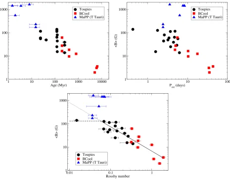
Figure 9. Trend in mean large-scale magnetic field strength with age, rotation period, convective turnover time, and Rossby number. Black circles are from our sample (the TOUPIES observational project), while red squares are additional field stars we consider from the BCool project. Blue triangles are TTS from the MaPP project. In the bottom panel, the solid line is the best-fitting power law, the dotted line is an extrapolation of this fit, and the dashed line is a hypothetical saturation value for the large-scale magnetic field. The TTS are fully convective, and are exceptions to the trends in rotation period and Rossby number.

the Metastable Dynamo Model. Additional planned observations of both faster and slower rotators, with ages extending up to 600 Myr, may provide additional constraints.

6.2 Comparison with older field stars

One of the limitations of our current sample is that it is still a modest size, and is focused mostly on young quickly rotating stars. Stronger conclusions can be drawn by adding older more slowly rotating stars from previous studies. We selected stars from the BCool sample (see Marsden et al.2014, for the first major paper in the series), which are mostly field MS stars with ages of a few Gyr. This is an excellent comparison sample, as the observations were obtained with the same instruments and observing strategy as our observations, and the same analysis techniques were used to derive magnetic maps for the stars. We specifically focus on stars in a similar mass range as our sample: 0.7–0.9 M_⊙, using the objects HD 22049 (ϵEri; Jeffers et al.2014), HD 131156A (ξBoo A; Petit et al.2005; Morgenthaler et al.2012), HD 131156B (ξBoo B; Petit et al., in preparation), HD 201091 (61 Cyg A; Boro Saikia et al., in preparation; Petit et al., in preparation), HD 101501, HD 10476,

HD 3651, HD 39587, and HD 72905 (Petit et al., in preparation). Ages for the stars are taken from Mamajek & Hillenbrand (2008) based on chromospheric activity. Since these stars are on the MS, and typically the younger half of the MS, H–R diagram ages are highly uncertain. The exception to this is HD 201091, where we use the more precise age of Kervella et al. (2008), based on an interferometric radius.

With these added stars, we see a much clearer trend in large-scale magnetic field strength with rotation period, as illustrated in Fig.9, while the trends in magnetic field strength with age and Rossby number are further supported. There is still no clear correla-tion between magnetic field strength and convective turnover time, largely because the BCool stars have the same range of turnover times as our sample. The added stars have a much stronger corre-lation between rotation period and age, since by these older ages the rotation rates of the stars have largely converged to a single sequence. The correlation of magnetic field strength with age and with rotation rate agree with the results from Vidotto et al. (2014); however, they considered a much larger mass range (from _∼0.2 to∼1.3 M_⊙), and some of our early results were included in that paper.