The Geometry of Optimal Control Solutions on some Six Dimensional Lie
Groups
James Biggs
School of Systems Engineering University of Reading,
Reading RG2, England Email:[email protected]
William Holderbaum
School of Systems Engineering University of Reading,
Reading RG2, England
Email:[email protected]
Abstract— This paper examines optimal solutions of control systems with drift defined on the orthonormal frame bundle of particular Riemannian manifolds of constant curvature. The manifolds considered here are the space forms Euclidean space E3
, the spheres S3
and the hyperboloids H3
with the corresponding frame bundles equal to the Euclidean group of motions SE(3), the rotation group SO(4) and the Lorentz group SO(1,3). The optimal controls of these systems are solved explicitly in terms of elliptic functions. In this paper, a geometric interpretation of the extremal solutions is given with particular emphasis to a singularity in the explicit solutions. Using a reduced form of the Casimir functions the geometry of these solutions are illustrated.
I. INTRODUCTION
This paper deals with affine control systems with drift defined on the frame bundles of simply connected manifolds of constant sectional curvature, denotedM. In particular the frame bundles of the space forms Euclidean space E3
, the spheresS3
and the hyperboloidsH3
with the corresponding frame bundles equal to the Euclidean group of motions
SE(3), the rotation group SO(4) and the Lorentz group
SO(1,3) respectively. Indeed E3
= SE(3)/SO(3), S3
=
SO(4)/SO(3) and H3
= SO(1,3)/SO(3). Orthonormal frame bundles of space forms coincide with their isometry group and therefore the focus shifts to control systems defined on Lie groups. The cotangent bundle T∗G is then realized as the product ofGwith the dual of its Lie algebra
g∗and leads to non-canonical coordinates, thus in this paper the use of the Maximum Principle of optimal control shifts the emphasis to 6-dimensional Hamiltonian systems defined on matrix Lie groups. Applications motivating this study are connected with controlling nonholonomic mechanical systems and in particular systems whose kinematics can be defined as affine control systems on Lie groups see, (see [1]). A simplified kinematic model of an airplane whose configuration can be described by SE(3) i.e it will always fly forward and the controls may yaw, pitch and roll the aircraft, has been used to find optimal landing trajectories for airplanes, (see [2]). The configuration SO(4) has a di-verse range of applications from such fields as mathematical physics (see [3]), to modelling power conversion in electrical circuits and in particular, Wood [4] has shown that switched electrical networks such as those used in power conversion
can be modelled as bilinear systems with state transition matrices that evolve on the Simple Orthogonal groupSO(n), where n is dependent on the number of capacitors and/or inductors in the circuit. In addition the spherical space form S3
can be used to represent spin systems in quantum control through the isomorphism S3
→SU(2). The Lorentz group has applications in physics and special relativity, indeed it is the isometry group of the 4-dimensional Minkowski metric. This paper explicitly solves for the optimal controls and the extremal solutions in terms of elliptic functions for the Euclidean, elliptic and hyperbolic case. In addition a geometric interpretation of these solutions is given using the invariant surfaces described by the Hamiltonian and Casimir functions. This illuminates the classical picture of elliptic curves as the intersection of quadric hypersurfaces in projective 3-space [5]. Finally, a geometric picture of the extremal solutions is given at a singularity of the system. At this singularity the solution is shown to be periodic and closed and the corresponding optimal controls trigonometric functions.
II. EXPLICIT SOLUTIONS ONse(3)∗,s0(4)∗ANDs0(1,3)∗ The groupGis used to represent the frame bundle of the space forms corresponding to the matrix Lie groupsSE(3),
SO(4)andSO(1,3)respectively. We identifyT GwithG×g
wheregis the Lie algebra of G and consider only the left translation. The elastic problem concern the solutions g(t)
of the left-invariant differential system
dg
dt(t) =g(t)(A0+
3 X
i=1
uiAi) (1)
whereA0, ..., A3 are given matrices in the Lie algebragof
Gand for our particular case (see [7] for a derivation):
dg
dt(t) =g(t)
0 −ε 0 0
1 0 −u3 u2
0 u3 0 −u1
0 −u2 u1 0
(2)
where ε=0 for the Euclidean case E3
, ε=1 for the elliptic caseS3
and ε=-1 for the hyperbolic case H3
. Equation (2) describes the deformations on the frame bundle G of M
° °dxdt
°
° = 1, and x is parameterized by its length from the initial point on the curve. In this optimal control problem we wish to minimize the expression 1
2 RT
0 (u(t)Qu(t))dt, subject to the given boundary condition g(0) = g0, g(T) = g1,Q
is diagonal and positive definite, and the diagonal entries will be denoted by ci’s. In the mechanics literature the ci’s are analogous to its principle moments of inertia and in the analogy to the elastic rod reflect the physical characteristics of the bar related to the geometric shape of its cross section [6]. Hereui play the role of the controls. It is interesting to note that ε coincides with the constant sectional curvature of the corresponding space form. In this sense ε can be viewed as a continuous parameter representing the curvature of an arbitrary Riemmanian manifold with constant curvature
ε. However, in this paper ε will be discrete and its value will distinguish between the three cases. The maximum principle of optimal control then identifies the appropriate left-invariant HamiltonianH on the dual of the Lie algebra
g∗, specificallyse(3)∗,so(4)∗ andso(1,3)∗. The maximum principle considers the lift of the optimization problem to the cotangent manifoldT∗G. The control Hamiltonian is written as:
H(p, g, u) =p(gA0) + 3 X
i=1
uip(gAi)−p0
1 2
3 X
i=1
ciu 2 i (3)
where p ∈ T∗
gG and p0 ∈ R is a constant of motion. The two cases where p0 is either 1 or 0, correspond to normal extremals and abnormal extremals respectively. That is there are two Hamiltonian functions to consider. Indeed, all these cases admit abnormal extremals. However, because of the regularity of these variational problems each optimal trajectory is a projection of a regular extremal curve (see [7]), therefore, we assumep0= 1. The Hamiltonian is defined on the cotangent manifold T∗G which can be pulled back to
G×g∗. The Hamiltonian function can be pulled back by the left or right action of an element g ∈G. Explicitly the pullback mapping by the left translated value can be defined as p(ˆ·) = p(g(·)) hence p(·) = ˆp(g−1
(·)). i.e p ∈ T∗G is pulled back to give a function pˆ∈g∗. Specifically, p(ˆ·) is defined via the non-degenerate Killing form on so(4) and
so(1,3). In the case of se(3) the trace form is degenerate but the functionp(ˆ·) is derived using a combination of the Euclidean inner product and the Killing form (see [7] for details). The control Hamiltonian ong∗ can be written as:
H(ˆp, u) = ˆp(A0) + 3 X
i=1
uip(Aˆ i)−
1 2
3 X
i=1
ciu 2
i (4)
The maximum principle states that the optimal controls u∗ will maximize the control Hamiltonian at every point of
T∗G. The control Hamiltonian is a quadratic function of the scalarui and d
2 H du2 i
<0 implies that there exists exactly one global maximum at each point of the Hamiltonian function. Differentiating (4) with respect to ui gives:
dH dui
= ˆp(Ai)−ciui
i= 1,2,3
(5)
Therefore, the optimal controls are defined in terms of the momentum functionp(ˆ·).
u∗
i =
1 ci
ˆ
p(Ai) (6)
wherei= 1,2,3. Also letp1= ˆp(A0)andMi= ˆp(Ai), then substituting these back into (4) gives the optimal Hamiltonian
H∗=p1+1
2
µ
M2 1
c1
+M
2 2
c2
+M
2 3
c3 
(7)
the optimal controls ui∗ can be substituted into (2) and rearranged to give
g−1dg
dt =
0 −ε 0 0
1 0 −M3/c3 M2/c2
0 M3/c3 0 −M1/c1
0 −M2/c2 M1/c1 0
(8)
In addition to the Hamiltonian defined on these groups it is also essential to recognize some geometric facts about these Lie algebras. Any element of these Lie algebras can be naturally split into two spacespandk, following the Cartan decomposition;g=p⊕k, which satisfy the classic relations.
[k,k]⊆k,[p,k]⊆p and[p,p]⊆k
wherekconsists of all matrices of the form
0 0 0 0
0 0 −a3 a2
0 a3 0 −a1
0 −a2 a1 0
(9)
andpconsists of the matrices
0 −εb1 −εb2 −εb3
b1 0 0 0
b2 0 0 0
b3 0 0 0
(10)
For notational convenience write the elementA0asB1. The corresponding adjoint representation forkandpwhereAi∈
kandBi∈p are:
A1=
0 0 0 0
0 0 0 0
0 0 0 −1
0 0 1 0
, A2=
0 0 0 0
0 0 0 1
0 0 0 0
0 −1 0 0
A3=
0 0 0 0
0 0 −1 0
0 1 0 0
0 0 0 0
, B1=
0 −ε 0 0
1 0 0 0
0 0 0 0
0 0 0 0
B2=
0 0 −ε 0
0 0 0 0
1 0 0 0
0 0 0 0
, B3=
0 0 0 −ε
0 0 0 0
0 0 0 0
1 0 0 0
[,] A1 A2 A3 B1 B2 B3
A1 0 A3 -A2 0 -B3 -B2
A2 -A3 0 A1 -B3 0 B1
A3 A2 -A1 0 B2 -B1 0
B1 0 B3 -B2 0 εA3 -εA2
B2 -B3 0 B1 -εA3 0 εA1
B3 B2 -B1 0 εA2 -εA1 0
Using the optimal Hamiltonian (7), it is possible to construct the Hamiltonian vector fields using the Poisson bracket de-fined on the symplectic manifold. The Poisson bracket is as-sociated with the Lie bracket by{Mi, Mj}=−p([Aˆ i, Aj]), wherepi= ˆp(Bi)andMi = ˆp(Ai)fori= 1,2,3. Therefore, deriving:
dM1
dt ={M1, H
∗}
={M1, p1}+
M1
c1
{M1, M1}+
M2
c2
{M1, M2}+
M3
c3
{M1, M3}= 0 + 0−
1 c2
M2M3+
1 c3
M3M2
= c2−c3 c2c3
M2M3
(12)
the remaining derivations of the Hamiltonian vector fields are left to the reader and yield:
dM1
dt ={M1, H
∗}= −M2M3
c2
+M2M3 c3
dM2
dt ={M2, H
∗}= M1M3
c1
−M1M3
c3
+p3
dM3
dt ={M3, H
∗}= −M1M2
c1
+M1M2 c2
−p2
dp1
dt ={p1, H
∗}= −M2p3
c2
+p2M3 c3
dp2
dt ={p2, H
∗}= M1p3
c1
−p1M3
c3
+εM3
dp3
dt ={p3, H
∗}=−M1p2
c1
+p1M2 c2
−εM2
(13)
where pi = ˆp(Bi). The Casimir functions are constant on co-adjoint orbits of G, they are integrals of motion for any left-invariant HamiltonianH. In addition the intersection of the surface described by the Casimir functions and the energy surface described by the Hamiltonian gives a geometric interpretation of the extremal solutions. A treatment of the three dimensional case is given in [8]. However, in the study of 6-dimensional Hamiltonian systems, there is an additional Casimir function. These are derived explicitly in [9] using the property that the Cartan-Killing form hL,·i=
−ε1
2T race(L,·) is invariant, where L is the projection of extremal solutions on the Lie algebra, specifically
L=
0 −εp1 −εp2 −εp3
p1 0 −M3 M2
p2 M3 0 −M1
p3 −M2 M1 0
(14)
then calculating hL, Li and hL2
, L2
i gives the Casimir functions I2 and I3 respectively. In the Euclidean case the Cartan-Killing form is non-degenerate, however, it is shown
in [10] that the Casimir functions can be derived using a combination of the Euclidean inner product on p and the Cartan-Killing form onk. The Hamiltonian and these Casimir functions are:
H =p1+
1 2( M2 1 c1 +M 2 2 c2 +M 2 3 c3 ) (15)
I2=p 2 1+p
2 2+p
2 3+ε(M
2 1 +M
2 2 +M
2
3) (16)
I3=p1M1+p2M2+p3M3 (17)
H,I2andI3are all constants of motion. Thus these functions are constant along the Hamiltonian flow and geometrically interpret hypersurfaces. The extremal solutions must exist on each of these surfaces and thus are defined at their intersection. For simplicity let c1 = c2 = c3 = 1 in (13), which is analogous to a particular case of the integrable Lagrange top in the Euclidean case, and immediately notice that
dM1
dt = 0 (18)
and thereforeM1 is a constant of motion denoted ask, the Hamiltonian vector fields (13) become
dM2
dt =p3 dM3
dt =−p2 dp1
dt =p2M3−M2p3 dp2
dt =p3k−M3p1+εM3 dp3
dt =p1M2−kp2−εM2
(19)
Therefore, the equations of motion in the Hamiltonian can be written in a reduced form. Proceeding to solve for the optimal controls:
dp1
dt =p2M3−M2p3
∴(dp
1
dt )
2
=p2 2M
2 3 +p
2 3M
2
2−2p2p3M2M3
(20)
Multiplying equation (15) by equation (16) write;
I2−p 2 1−ε(k
2
) =p2 2+p
2 3+ε(M
2 2 +M
2 3)
2(H−p1)−k 2
=M2 2+M
2 3
∴(I2−p 2 1−ε(k
2
))(2(H−p1)−k 2
) =p2
2M 2 2 +p
2 2M
2 3+p
2 3M
2 2+p
2 3M
2
3 +ε((M 2 2+M
2 3)
2
)
(21) Another useful relation comes from the Casimir function (17), writing this in a reduced form and squaring gives:
I3−p1k=p2M2+p3M3
∴(I3−p1k) 2
=p2 2M
2 2+p
2 3M
2
3 + 2p2M2p3M3 (22)
Therefore, substituting (22) and (21) into (20) yields:
f(p1) = (
dp1
dt )
2
= (I2−p 2 1−ε(k
2
))(2(H−p1)−k 2
)
−(I3−p1k) 2
−ε((2H−k2 −2p1)
2
)
The function f(p1) is then a cubic function of p1 and the qualitative behavior of the system will depend on where the roots of this cubic lie. Explicit solutions of (23) can be solved in terms of elliptic functions, see [11] and [2]. Proceeding to solve forM2 andM3using the Casimir function (15) where
M1is a constant k, the reduced Casimir is:
M2 2 +M
2
3 = 2(H−p1)−k 2
(24)
This suggests using polar coordinates forM2andM3(M36=
0);
θ= arctan
µ
M2
M3 
(25)
·
θ=M3
·
M2−M2 ·
M3
M2 2+M
2 3
(26)
substituting in the values forM2andM3 from (19) gives
·
θ= M3p3−M2p2 M2
2 +M 2 3
= I3−kp1 2(H−p1)−k2
(27)
Solving explicitly for the radius in (24) gives:
r=p2(H−p1)−k2 (28)
so, the optimal controls are
M1(t) =k
M2(t) =r(t) cos(θ(t))
M3(t) =r(t) sin(θ(t))
(29)
Note that ifp1 is constant in (27) and (28) then the optimal controls M2 and M3 in (29) degenerate to trigonometric functions (a geometric interpretation of the extremal solu-tions at these singularities is given in Section (III)). With the
M1constant denoted k, the Casimir functions reduce to:
H−1
2k
2
=p1+
1 2(M
2 2+M
2
3) (30)
I2−εk 2
=p2 1+p
2 2+p
2 3+ε(M
2 2 +M
2
3) (31)
I3−k=
p2M2+p3M3
p1
(32)
The left hand side of the equations (30), (31) and (32) are constants and thus a reduced form of the Casimir functions. Each of these equations implicitly describe an invariant surface. (30) describes an elliptic paraboloid, (31) describes the sphere for ε=0, the 6-dimensional sphere for ε=1 and finally a non-generic 5-dimensional surface for ε=-1. The Casimir function (32) also implicitly defines a non-generic 5-dimensional surface. It is possible to write the two Casimir functions as a single surface. Rearranging (32) in terms of
p2, squaring and substituting in (31) gives:
1 M22
(εM2 2(k
2
+M2 2 +M
2 3) +I
2 3p
2 1+k
2
p2 1+M
2 2p
2 1
+2kM3p1p3+M 2 2p
2 3+M
2 3p
2
3−2I3p1(kp1+M3p3)) =I2 (33)
This is a 4-dimensional hypersurface and the intersection of this with the Hamiltonian function (30) gives us the extremal solutions. It is interesting to note that a classical picture of an elliptic curve is the smooth intersection of two quadric hypersurfaces in projective three space [5]. In the Euclidean case where ε = 0, the Hamiltonian and the function (33) implicitly define two quadric surfaces and the extremal solutions can be expressed in terms of elliptic curves, reinforcing the classical picture. In the non-Euclidean case the hypersurface (33) is not a quadric, although the explicit solutions are in terms of elliptic functions.
III. DEGENERATE SOLUTIONS ONse(3)∗,so(4)∗,
so(1,3)∗AND THEIR GEOMETRY
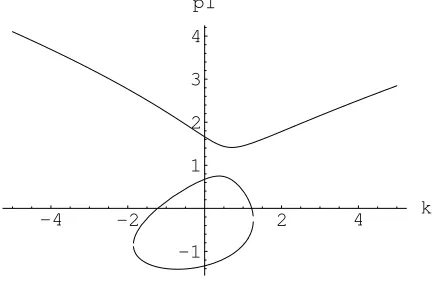
Recall that p1 is a solution of the cubic equation (23). There is a qualitative difference in the solutions depending on where the three roots of the cubic lie. At any one of these roots the solutions for the optimal controls degenerate from elliptic functions to trigonometric functions asp1is constant. A plot of the real roots (singularities) are given in Fig.(1) for
ε= 0. The figure illustrates the real roots p1 as a function ofk.
-4 -2 2 4 k
[image:4.612.326.544.338.484.2]-1 1 2 3 4 p1
Fig. 1. The singularities of the systemε=0
Forε=1 andε=-1, the analysis is also restricted to the real roots of the cubic (23). Continuing to study the system when
p1 is constant and denoting this constant as c, the Casimir functions (15), (16) and (17) reduce further to:
2(H−c)−k2
=M2 2 +M
2
3 (34)
I2−c 2
−ε(k2
) =p2 2+p
2 3+ε(M
2 2 +M
2
3) (35)
I3−ck=p2M2+p3M3 (36)
where the left hand side of these equations are all constants along the Hamiltonian flow. Expressing equation (36)in terms ofp2 and squaring gives;
p2 2=
(I2
3−2I3ck+c 2
k2
)−2I3p3M3+ 2ckp3M3+p 2 3M
2 3
M2 2
(37) defining new constants α= (I2
3 −2I3ck+c2k2) and β =
the reduced Casimir function can be written as a non-generic quadric surface inp3, M2 andM3, giving:
2(H−c)−k2
=M2 2 +M
2 3
βM2
2 =α+p 2 3M
2
2 + 2ckp3M3−2I3p3M3
+p2 3M
2 2 +ε(M
4 2 +M
2 2M
2 3)
(38)
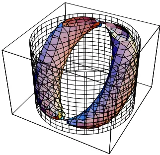
[image:5.612.350.515.51.200.2]Proceeding more geometrically we analyze the solutions in terms of the intersection of these two invariant surfaces. It is necessary for illustration purposes to consider only the critical values of p1 that are real and give a positive reduced Hamiltonian (the left hand side of the first equation in (38) is positive). In these cases the Hamiltonian invariant surface (cylinder), intersects the reduced Casimir surface (non-generic) see Fig.(2) for ε = 0, Fig.(3) for ε = 1 and Fig.(4) for ε = −1. In all of these cases the vertical axis is the p3 variable, and the horizontal axis are M2 and M3 respectively:
Fig. 2. The Euclidean case: intersection of invariant surfaces
[image:5.612.98.254.300.499.2]Fig. 3. The elliptic case: intersection of invariant surfaces
Fig. 4. The hyperbolic case: intersection of invariant surfaces
These surfaces were drawn using ImplicitPlot3D code written by Steven Wilkinson for Mathematica see
http://library.wolfram.com/infocenter/MathSource/4189/
and as the name suggests enables one to plot surfaces that are implicitly defined in 3 dimensions. The surfaces make contact and in each case the intersection is a closed periodic orbit. Fig.(5) shows the points of intersection for ε = 0, this remains qualitatively unchanged in each caseε= 1and
ε=−1.
-1
0
1
M2 -1
0 1
M3 -0.5
0 0.5
p3
-1
0
[image:5.612.357.516.375.506.2]1 M2
Fig. 5. Closed periodic orbit; intersection of invariant surfaces
At this singularity (dp1dt = 0) the Hamiltonian vector fields (19) reduce to;
dM2
dt =p3 dM3
dt =−p2 dp2
dt =kp3−cM3+εM3 dp3
dt =cM2−kp2−εM2 dp1
dt = 0⇒p2= M2p3
M3
(39)
[image:5.612.95.256.555.711.2] [image:5.612.383.494.595.714.2]can be expressed independently ofp2 as
dM2
dt =p3 dM3
dt =−
M2p3
M3
dp3
dt =M2(c−k p3
M3 −ε)
(40)
Changing the initial conditions to perturb away from the periodic orbit will mean that the constantp1=cwill have to change if it is to remain a constant, i.e. the Casimir functions (34), (35) and (36) constrain the flow. The radius (28) will then change accordingly and the extremal solution will again be a closed periodic orbit with a different radius. From (40) it is deduced that the flow of these closed periodic orbits are in a clockwise direction. From (40) it can be seen that there is a fixed point at p3=M2= 0, this corresponds to the explicit solutions whenr= 0in (28) i.e.2(H−p1)−k2= 0, in other words when the reduced Hamiltonian is zero the periodic orbit degenerates to a fixed point. Perturbing away from the periodic orbit such thatp1 does not change accordingly to remain a constant, then p1 will be an elliptic function. Consequently the dynamics will then be described by the Hamiltonian vector fields (19).
IV. CONCLUSION
The optimal controls and the extremal solutions for these systems are explicitly solved in terms of elliptic functions using the Hamiltonian formalism of Pontryagin’s maximum principle. In addition it is shown that at a real singularity of the system with positive Hamiltonian function the optimal controls degenerate from elliptic to trigonometric functions. This is an interesting case as it shows that trigonometric controls are in some sense optimal. Indeed trigonometric functions have been used to control systems for the Euclidean group of motionSE(3), (see [1]). The elliptic solutions are shown to correspond to the intersection of hypersurfaces and in particular, for the Euclidean case the intersection of quadric hypersurfaces in projective 3 space illucidates the classical picture of elliptic curves. Finally, a geometric picture of the extremal solutions at a singularity is given and is shown to be the intersection of the reduced Hamiltonian function (cylinder) and a non-generic quadric dependent on
ε. At this singularity the extremal solutions are shown to be periodic and closed. The differential equations describing these periodic orbits can be interpreted as a constrained dynamical system embedded in a higher dimension Hamil-tonian system. Current and future research concerns the corresponding elastic curves in the base spaces E3
, S3 and H3
when the optimal controls are trigonometric functions.
REFERENCES
[1] N. E. Leonard, “Averaging and motion control of systems on lie groups,”PhD thesis, University of Maryland,College Park,MD, 1994. [2] G. W. R. Montgomery and S. Sastry, “Optimal path planning on matrix lie groups,”Proceedings of IEEE Conference on Decision and Control, 1994.
[3] O. Bogoyavlensky, “Integrable euler equations on so(4) and their phys-ical applications,”Communications in Mathematical Physics, vol. 93, pp. 417–436, 1984.
[4] J. R. Wood, “Power conversions in electrical networks,” Technical Report NASA Rep. No. CR-120830, Phd Thesis, Harvard University, 1974.
[5] D. Husemoller,Elliptic Curves. Springer-Verlag , New York, 2000. [6] V. Jurdjevic,Geometric Control Theory, Advanced Studies in
Mathe-matics Vol. 52. Cambridge University Press, 1997.
[7] V.Jurdjevic and F. Monroy-Perez,Lie Systems in Control Theory in Contemporary Trends in Nonlinear Geometric Control Theory. World Scientific, 2002.
[8] V. Jurdjevic, “Non-euclidean elastica,”American Journal of Mathe-matics, vol. 117, pp. 93–125, 1995.
[9] ——, Optimal Control Problems on Lie Groups, B. Jakubczyk and W. Respondek, editors, Geometry of Feedback and Optimal Control. Marcel-Dekker, 1992.
[10] ——, “Integrable hamiltonian systems on complex lie groups,” to appear in American Journal of Mathematics, 2005.