Rochester Institute of Technology
RIT Scholar Works
Theses
Thesis/Dissertation Collections
9-1-2008
Statistical modeling of radiometric error
propagation in support of hyperspectral imaging
inversion and optimized ground sensor network
design
Scott Klempner
Follow this and additional works at:
http://scholarworks.rit.edu/theses
This Dissertation is brought to you for free and open access by the Thesis/Dissertation Collections at RIT Scholar Works. It has been accepted for inclusion in Theses by an authorized administrator of RIT Scholar Works. For more information, please [email protected].
Recommended Citation
Statistical Modeling of Radiometric Error Propagation in
Support of Hyperspectral Imaging Inversion and Optimized
Ground Sensor Network Design
by
Scott Klempner
B. S. United States Air Force Academy, 1998
M. Eng. University of Colorado, 1999
A dissertation submitted in partial fulfillment of the
requirements for the degree of Doctor of Philosophy
in the Chester F. Carlson Center for Imaging Science
Rochester Institute of Technology
4 September 2008
Signature of the Author
Accepted by
CHESTER F. CARLSON CENTER FOR IMAGING SCIENCE
ROCHESTER INSTITUTE OF TECHNOLOGY
ROCHESTER, NEW YORK
CERTIFICATE OF APPROVAL
Ph.D. DEGREE DISSERTATION
The Ph.D. Degree Dissertation of Scott Klempner has been examined and approved by the dissertation committee as satisfactory for the
dissertation required for the Ph.D. degree in Imaging Science
Dr. John R. Schott, dissertation Advisor
Dr. John P. Kerekes
Dr. Peter Bajorski
Dr. Steven M. LaLonde
Date
Title of thesis or dissertation: ____________________________________________________ ____________________________________________________________________________ ____________________________________________________________________________ ____________________________________________________________________________
Name of author: _______________________________________________________________ Degree: ____________________________________________________________________ Program: ____________________________________________________________________ College: ____________________________________________________________________
I understand that I must submit a print copy of my thesis or dissertation to the RIT Archives, per current RIT guidelines for the completion of my degree. I hereby grant to the Rochester Institute of Technology and its agents the non-exclusive license to archive and make accessible my thesis or dissertation in whole or in part in all forms of media in perpetuity. I retain all other ownership rights to the copyright of the thesis or dissertation. I also retain the right to use in future works (such as articles or books) all or part of this thesis or dissertation.
Print Reproduction Permission Granted:
I, __________________________________, hereby grant permission to the Rochester Institute
Technology to reproduce my print thesis or dissertation in whole or in part. Any reproduction will not be for commercial use or profit.
Signature of Author: ________________________________________ Date: ____________
Print Reproduction Permission Denied:
I, __________________________________, hereby deny permission to the RIT Library of the Rochester Institute of Technology to reproduce my print thesis or dissertation in whole or in part.
Signature of Author: ________________________________________ Date: ____________
Inclusion in the
RIT Digital Media Library Electronic Thesis & Dissertation (ETD) Archive
I, __________________________________, additionally grant to the Rochester Institute of Technology Digital Media Library (RIT DML) the non-exclusive license to archive and provide electronic access to my thesis or dissertation in whole or in part in all forms of media in perpetuity.
I understand that my work, in addition to its bibliographic record and abstract, will be available to the world-wide community of scholars and researchers through the RIT DML. I retain all other ownership rights to the copyright of the thesis or dissertation. I also retain the right to use in future works (such as articles or books) all or part of this thesis or dissertation. I am aware that the Rochester Institute of Technology does not require registration of copyright for ETDs.
I hereby certify that, if appropriate, I have obtained and attached written permission statements from the owners of each third party copyrighted matter to be included in my thesis or dissertation. I certify that the version I submitted is the same as that approved by my committee.
Signature of Author: _____________________________ Date: ____________ Statistical Modeling of Radiometric Error
Scott Klempner Doctor of Philosophy Imaging Science College of Science
Scott Klempner
Scott Klempner
Statistical Modeling of Radiometric Error Propagation in
Support of Hyperspectral Imaging Inversion and Optimized
Ground Sensor Network Design
by
Scott Klempner
Submitted to the
Chester F. Carlson Center for Imaging Science in partial fulfillment of the requirements
for the Doctor of Philosophy Degree at the Rochester Institute of Technology
Abstract
A method is presented that attempts to isolate the relative magnitudes of various er-ror sources present in common algorithms for inverting the effects of atmospheric scattering and absorption on solar irradiance and determine in what ways, if any, operational ground truth measurement systems can be employed to reduce the over-all error in retrieved reflectance factor. Error modeling and propagation methodol-ogy is developed for each link in the imaging chain, and representative values are determined for the purpose of exercising the model and observing the system be-havior in response to a wide variety of inputs. Three distinct approaches to model-based atmospheric inversion are compared in a common reflectance error space, where each contributor to the overall error in retrieved reflectance is examined in relation to the others. The modeling framework also allows for performance predic-tions resulting from the incorporation of operational ground truth measurements. Regimes were identified in which uncertainty in water vapor and aerosols were each found to dominate error contributions to final retrieved reflectance. Cloud cover was also shown to be a significant contributor, while state-of-the-industry hyperspectral sensors were confirmed to not be error drivers. Accordingly, instru-ments for measuring water vapor, aerosols, and downwelled sky radiance were identified as key to improving reflectance retrieval beyond current performance by current inversion algorithms.
Acknowledgements
I wish to express gratitude toward Dr. Schott and my dissertation committee. Their guidance was invaluable and forbearance necessary as I finished this work from three states and 380 miles away. Likewise, I wish to sincerely thank Cindy Schultz for making this long distance relationship work. Every time I worked with her to get closer to this finish point, it was personally encouraging to me, and there were times it was really needed. I feel if I attempted to capture on printed page all the praise she really deserves, it might double the length of this document.
After leaving Rochester and moving to Virginia, I encountered a whole new group of people who offered continual support and encouragement, especially Eleanor, Tiina, Brett, and the Colonels. I greatly appreciated it.
I would like to especially thank my wife Amy. Not only is she the nicest person I know, she has also endured far more than any spouse should have to, even if it is common in this line of work. She was only expecting three years of school-induced separation, and I handed her five. The two most important phrases in a marriage seem apropos here: I’m sorry, and I love you. Thank you.
I would like to thank my partners Brent Bartlett and Brian Daniel for their spe-cial assistance in the field research of operationally deployed atmospheric sounding systems and hydrodynamic power generation.
Finally, thanks to Jake Ward for always taking the outside lane.
For Patrick, Colin, Will, and Sean
Contents
1 Introduction 1
2 Objectives 9
2.1 Main Objectives . . . 9
2.2 Minor Objectives . . . 10
2.3 Scope . . . 11
2.4 Success Criteria . . . 12
3 Background 15 3.1 Radiative transfer model . . . 15
3.2 Inversion algorithm descriptions . . . 19
3.2.1 Empirical algorithm: the Empirical Line Method . . . 21
3.2.2 Model-based algorithm: Green’s method . . . 25
3.2.3 Model-based algorithm: Fast Line-of-Sight Atmospheric Analysis of Spectral Hypercubes (FLAASH) . . . 28
4 Approach and Theory 31 4.1 Introduction . . . 31
4.2 Imaging operators . . . 32
4.3 Forward uncertainty model description . . . 33
4.4 Error propagation in analytical functions . . . 36
4.4.1 Total error . . . 36
4.4.2 Random component . . . 38
4.4.3 Bias component . . . 40
4.5 Governing equation . . . 41
4.6 Application of error propagation . . . 44
4.6.1 Main equations . . . 44
4.6.2 Correlation coefficients . . . 45
xii CONTENTS
4.6.3 Partial derivatives . . . 47
4.6.4 Bias terms . . . 48
4.7 Numerically-determined derivatives . . . 50
4.7.1 General equations . . . 51
4.7.2 Error considerations . . . 53
4.8 Slope calculation using MODTRAN . . . 55
4.9 Uncertainty in atmospheric parameters . . . 57
4.9.1 Error sources from climatology . . . 58
4.9.2 Error sources from ground instruments . . . 60
4.9.3 Error sources from inversion algorithms . . . 60
4.10 Total atmospheric error . . . 61
4.11 Physical models . . . 61
4.11.1 Elevation knowledge . . . 62
4.11.2 Exoatmospheric solar irradiance . . . 63
4.12 Sensor error models . . . 65
4.12.1 Radiometric calibration . . . 66
4.12.2 Spectral calibration . . . 67
4.12.3 Ground radiometer . . . 71
4.12.4 Mechanical factors . . . 74
4.13 Environmental error models . . . 75
4.13.1 Target tilt . . . 76
4.13.2 Clouds . . . 79
4.13.3 Background objects . . . 87
4.13.4 Pointing . . . 93
4.14 Scenario setup . . . 97
4.15 Validation . . . 99
5 Results and Discussion 103 5.1 Atmospheric partial derivatives . . . 105
5.1.1 Step size selection . . . 105
5.1.2 Slope determination in MODTRAN functional space . . . 106
5.2 Atmospheric constituent uncertainty . . . 113
5.2.1 Constituents from Climatology . . . 114
5.2.2 Constituents from Instrumentation . . . 115
5.2.3 Constituents from In-scene Algorithms . . . 116
5.2.4 Atmospheric Constituent Scenarios . . . 124
5.3 Error in Modeling Outputs . . . 124
CONTENTS xiii
5.4.1 Radiometric precision . . . 125
5.4.2 Radiometric accuracy . . . 128
5.4.3 Spectral calibration . . . 128
5.5 Environmental error modeling results . . . 135
5.5.1 Pointing angle modeling results . . . 136
5.5.2 Cloud modeling results . . . 138
5.5.3 Background object modeling results . . . 140
5.5.4 Environmental error scenario summary . . . 141
5.5.5 Combined effects . . . 141
5.6 Total error . . . 142
5.6.1 Scenario 1 – Climatological sources . . . 144
5.6.2 Scenario 2 – Field-quality ground instruments . . . 146
5.6.3 Scenario 3 – Research quality ground instruments . . . 147
5.6.4 Scenarios 4 and 5 – In-scene sources . . . 147
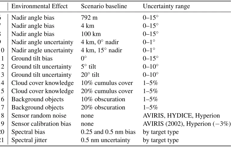
5.6.5 Scenarios 6 through 8 – Off-nadir pointing bias . . . 149
5.6.6 Scenarios 9 and 10: Off-nadir pointing uncertainty . . . . 150
5.6.7 Scenario 11: Ground tilt bias . . . 150
5.6.8 Scenarios 12–13: Ground tilt knowledge uncertainty . . . 150
5.6.9 Scenarios 14–17: Bias error due to cloud cover and back-ground objects . . . 151
5.6.10 Scenario 18: Sensor noise . . . 153
5.6.11 Scenario 19: Sensor radiometric calibration bias . . . 153
5.6.12 Scenario 20: Bias error due to spectral misregistration . . 155
5.6.13 Scenario 21: Spectral jitter uncertainty . . . 156
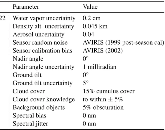
5.6.14 Final Scenario: Mean squared error for combined effects . 157 5.7 Validation . . . 165
5.8 Error sensitivity study . . . 167
5.8.1 Scenario 1 . . . 168
5.8.2 Explanation of counterintuitive results . . . 169
5.8.3 Scenarios 2 and 3 . . . 172
5.8.4 Scenario 4 . . . 173
5.8.5 Scenario 5 . . . 173
5.8.6 Direct measurement ofτ1andLd . . . 174
5.9 Optimal network design . . . 176
xiv CONTENTS
6 Conclusions and Future Work 185
6.1 Modeling Work and System Behavior . . . 185
6.2 Future Work . . . 189
A Full Expressions for Selected Equations 191 A.1 Partial derivatives of reflectance . . . 191
A.2 Correlation and error terms . . . 193
A.3 Consolidated expressions . . . 196
A.4 Digital elevation model altitude error . . . 199
B Climatology Analysis Results 201
C Environmental Effect Modeling Results 207
D Atmospheric Uncertainty Results 217
E Environmental Effect Results 229
F Validation Results 243
G Error Improvement Sensitivity Results 263
H Atmospheric Derivative Functional Spaces 285
List of Figures
1.1 Early satellite imagery . . . 2
1.2 LandSAT VII diagram . . . 3
1.3 Unattended sensor network . . . 4
3.1 Indirect radiance sources . . . 18
3.2 Sky fraction naming convention . . . 20
3.3 The linear relationship of the empirical line method . . . 22
3.4 ELM uncertainty . . . 23
3.5 ELM linear regression . . . 24
3.6 760 nm oxygen feature variation with sensor altitude . . . 26
3.7 Water vapor absorption features by total column amount . . . 27
4.1 Imaging operator block diagram . . . 33
4.2 Target/image space model . . . 34
4.3 Forward uncertainty chain . . . 35
4.4 Three-level uncertainty chain block diagram . . . 36
4.5 Antecedent sources in the modeling chain . . . 44
4.6 Chebyshev curve fit slope error . . . 53
4.7 A comparison of systematic and functional error . . . 54
4.8 Construction of total error in each model output . . . 61
4.9 DEM interpolation visualization . . . 62
4.10 DEM altitude error using SRTM values and flat terrain . . . 63
4.11 Illustration of spectral calibration errors and their effects on the imaging chain . . . 68
4.12 Percent error in radiance as a function of band center shift . . . . 70
4.13 Reflectance curves used to simulate spectral cal errors . . . 71
4.14 Radiance curves used to simulate spectral cal errors . . . 72
4.15 Ground reflectometer in dual-input configuration . . . 73
xvi LIST OF FIGURES
4.16 Tilted target relative to the local horizon . . . 76
4.17 Elevation measurement scenario . . . 77
4.18 DEM interpolation error in elevation . . . 78
4.19 DEM interpolation error in direct solar term . . . 78
4.20 Cloud concepts . . . 81
4.21 Clear-sky radiance results for 72 and 1224 quads . . . 83
4.22 Radiance sources for a background object . . . 88
4.23 Background radiance, measured vs predicted . . . 90
4.24 Quad integration approach for background objects . . . 91
4.25 Azimuthal variation in simulated background objects . . . 92
4.26 Nadir and off-nadir pointing terms . . . 94
4.27 Upwelled radiance by azimuth and nadir angle . . . 95
4.28 Variation inLuandτ2by pointing angle, relative to nadir . . . 96
5.1 Map of Component Results . . . 104
5.2 Water vapor slope step size sensitivity . . . 107
5.3 Altitude slope step size sensitivity . . . 108
5.4 Aerosol/Visibility slope step size sensitivity . . . 109
5.5 Derived slopes forτ1 . . . 111
5.6 Derived slopes forτ2 . . . 111
5.7 Derived slopes forLd . . . 112
5.8 Derived slopes forLu . . . 112
5.9 Relationship between aerosol optical depth and visibility . . . 113
5.10 CIBR and APDA validation results . . . 121
5.11 Sample results for error in modeling outputs . . . 126
5.12 Instrument radiometric calibration noise models . . . 129
5.13 Reflectance retrieval from Hyperion imagery . . . 130
5.14 AVIRIS radiometric calibration bias . . . 131
5.15 Hyperion radiometric calibration bias . . . 132
5.16 Radiance bias error due to spectral misregistration . . . 133
5.17 Standard deviation in percent radiance error . . . 134
5.18 Uncertainty in radiance due to 0.5 nm spectral jitter . . . 136
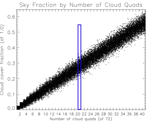
5.19 Relationships between cloud quads and sky fraction . . . 139
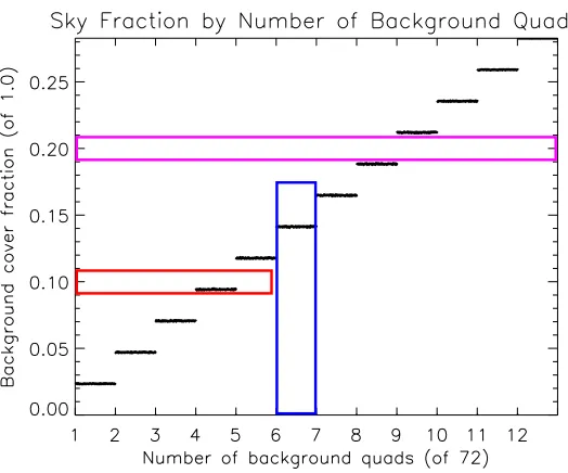
5.20 Correlation between background quads and sky fraction . . . 141
5.21 Total reflectance uncertainty summary for basic scenarios 1-5 . . . 145
5.22 940 nm absorption feature . . . 156
5.23 Bias in retrieved CIBR water vapor . . . 157
LIST OF FIGURES xvii
5.25 Background reflectance bias for final scenario . . . 159
5.26 Total reflectance bias error for final scenario . . . 159
5.27 Final scenario mean squared error . . . 160
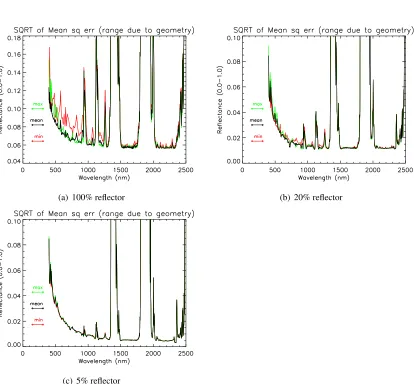
5.28 Square root of mean squared error for the final scenario (with geo-metric variability for clouds and background objects) . . . 162
5.29 Final scenario variant mean squared error . . . 163
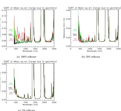
5.30 Square root of mean squared error for the final scenario (with geo-metric variability for clouds and background objects) . . . 164
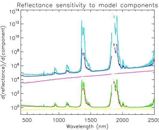
5.31 Reflectance uncertainty sensitivity . . . 171
5.32 Instrument Tradeoff Matrix . . . 179
B.1 GPS-based climate model for water vapor . . . 201
B.2 Radiosonde-based climate model for water vapor . . . 202
B.3 MODIS-based climate model for water vapor . . . 202
B.4 Airport observation-based climate model for density altitude . . . 203
B.5 GPS-based climate model for density altitude . . . 203
B.6 Radiosonde-based climate model for density altitude . . . 204
B.7 MODIS-based climate model for aerosols . . . 204
B.8 Airport observation-based climate model for visibility . . . 205
B.9 Airport observation-based visibility histogram . . . 205
C.1 Off-nadir pointing effects, sensor at 792 m . . . 208
C.2 Off-nadir pointing effects, sensor at 4 km . . . 209
C.3 Off-nadir pointing effects, sensor at 11 km . . . 210
C.4 Off-nadir pointing effects, sensor at 100 km . . . 211
C.5 Multiple scattering algorithm effect on off-nadir pointing . . . 212
C.6 Cumulus cloud modeling results . . . 213
C.7 Cloud type comparison . . . 214
C.8 Background modeling results . . . 215
D.1 Legend for reflectance results . . . 218
D.2 Legend for correlation results . . . 218
D.3 Scenario 1 – reflectance error . . . 219
D.4 Scenario 1 – correlations . . . 220
D.5 Scenario 2 – reflectance error . . . 221
D.6 Scenario 2 – correlations . . . 222
D.7 Scenario 3 – reflectance error . . . 223
D.8 Scenario 3 – correlations . . . 224
xviii LIST OF FIGURES
D.10 Scenario 4 – correlations . . . 226
D.11 Scenario 5 – reflectance error . . . 227
D.12 Scenario 5 – correlations . . . 228
E.1 Scenarios 6-8, off-nadir pointing bias error, 100% reflector . . . . 230
E.2 Scenarios 6-8, off-nadir pointing bias error, 20% reflector . . . 231
E.3 Scenarios 9-10, off-nadir pointing random error . . . 232
E.4 Scenario 11, ground tilt bias error . . . 233
E.5 Scenarios 12-13, ground tilt random error, 100% reflector . . . 234
E.6 Scenarios 14-15, cloud bias error, 100% reflector . . . 235
E.7 Scenarios 14-15, cloud bias error, 20% reflector . . . 236
E.8 Scenarios 16-17, background object bias error, 100% reflector . . 237
E.9 Scenarios 16-17, background object bias error, 20% reflector . . . 238
E.10 Scenario 18, sensor noise random error . . . 239
E.11 Scenario 19, sensor radiometric calibration bias error . . . 240
E.12 Scenario 20, retrieved reflectance bias error due to spectral misreg-istration . . . 241
E.13 Scenario 21, uncertainty in retrieved reflectance due to 0.5 nm spectral jitter . . . 242
F.1 Validation scenario 1 – 100% reflector . . . 244
F.2 Validation scenario 1 – 20% reflector . . . 245
F.3 Validation scenario 2 – 100% reflector . . . 246
F.4 Validation scenario 2 – 20% reflector . . . 247
F.5 Validation scenario 3 – 100% reflector . . . 248
F.6 Validation scenario 3 – 20% reflector . . . 249
F.7 Validation scenario 4 – 100% reflector . . . 250
F.8 Validation scenario 4 – 20% reflector . . . 251
F.9 Validation scenario 5 – 100% reflector . . . 252
F.10 Validation scenario 5 – 20% reflector . . . 253
F.11 Validation scenario 6 – 100% reflector . . . 254
F.12 Validation scenario 6 – 20% reflector . . . 255
F.13 Validation scenario 7 – 100% reflector . . . 256
F.14 Validation scenario 7 – 20% reflector . . . 257
F.15 Validation scenario 8 – 100% reflector . . . 258
F.16 Validation scenario 8 – 20% reflector . . . 259
F.17 Validation scenario 9 – 100% reflector . . . 260
LIST OF FIGURES xix
G.1 Legend for error sensitivity results . . . 263
G.2 Scenario 1 –a prioriknowledge climatology inputs . . . 264
G.3 Scenario 1 – multiple reflectance comparison . . . 265
G.4 Scenario 1 – aerosol individual results . . . 266
G.5 Scenario 1 – water vapor individual results . . . 267
G.6 Scenario 2 – inputs from commercial quality instrumentation . . . 268
G.7 Scenario 2 – multiple reflectance comparison . . . 269
G.8 Scenario 2 – aerosol individual results . . . 270
G.9 Scenario 2 – water vapor individual results . . . 271
G.10 Scenario 3 – inputs from ARM-grade instrumentation . . . 272
G.11 Scenario 3 – multiple reflectance comparison . . . 273
G.12 Scenario 3 – aerosol individual results . . . 274
G.13 Scenario 3 – water vapor individual results . . . 275
G.14 Scenario 4 –a prioriknowledge climatology inputs . . . 276
G.15 Scenario 4 – multiple reflectance comparison . . . 277
G.16 Scenario 4 – aerosol individual results . . . 278
G.17 Scenario 4 – water vapor individual results . . . 279
G.18 Scenario 5 –a prioriknowledge climatology inputs . . . 280
G.19 Scenario 5 – multiple reflectance comparison . . . 281
G.20 Scenario 5 – aerosol individual results . . . 282
G.21 Scenario 5 – water vapor individual results . . . 283
H.1 Derivative∂τ1/∂alt. . . 286
H.2 Derivative∂τ1/∂vis . . . 286
H.3 Derivative∂τ1/∂H2O . . . 287
H.4 Derivative∂τ2/∂vis . . . 287
H.5 Derivative∂τ2/∂alt. . . 288
H.6 Derivative∂τ2/∂H2O . . . 288
H.7 Derivative∂Ld/∂vis . . . 289
H.8 Derivative∂Ld/∂H2O . . . 289
H.9 Derivative∂Ld/∂alt . . . 290
H.10 Derivative∂Lu/∂vis . . . 290
H.11 Derivative∂Lu/∂alt . . . 291
List of Tables
4.1 Baseline Scenario Geometry . . . 98 4.2 Baseline Sensor Parameters . . . 98 4.3 Baseline MODTRAN Atmospheric Parameters . . . 98 4.4 Other Selectable Parameters . . . 99 4.5 Validation scenario summary . . . 102
5.1 Partial Derivative Settings Summary . . . 105 5.2 Climatology Results Summary (Month 5) . . . 115 5.3 Temperature . . . 116 5.4 Pressure . . . 117 5.5 Aerosol Optical Depth . . . 117 5.6 Water Vapor . . . 121 5.7 Inversion algorithm constituent determination summary . . . 124 5.8 Atmospheric Uncertainty Scenario Settings . . . 125 5.9 Environmental Error Scenario Settings . . . 142 5.10 Combined Effect Scenario Settings . . . 143 5.11 Validation scenario summary . . . 165 5.12 Instrument improvement analysis (averaged over visible bands) . . 178
Chapter 1
Introduction
The story of remote sensing has been one of steady technological innovation, evolving image processing and data extraction techniques, and branching appli-cations. Each new generation of technology builds on needs that have emerged from the previous generation’s remote sensing applications and data processing methods and, in turn, prompts new application branches and new data extraction capabilities. Taking photographs from a balloon, first documented in 1858, pre-dates the US Civil War, and this capability led to the employment of battlefield surveillance techniques during the war. The invention of the first modern cam-era in 1888 (including flexible rolled film and standardized chemical processing) and powered flight shortly thereafter enabled the first true aerial photography, em-ployed in World War I and II. The invention of color infrared film not only had applications in detecting camouflage but also vegetation health. This discovery in the mid-1950’s established the utility of remote sensing in agricultural research (Campbell, 1987).
The spiral evolution of remote sensing has continued with satellite photogra-phy, digital imaging, multispectral, multitemporal, and most recently hyperspec-tral imaging. The Corona project, the existence of which was made public in 1995, marked the first time remote sensing was conducted from space - the result of which is shown in figure 1.1. This excerpt from a 1960 memorandum to the US Intelli-gence Board illustrates the relationship between needs, technology, applications, and exploitation:
For six years the U. S. intelligence agencies have had extensive ex-perience with the larger scale photography from overflight held in the [redacted] and TALENT Systems. New equipment bearing upon the art of photographic interpretation has clearly expanded the quantity
2 CHAPTER 1. INTRODUCTION
and quality of information derived from that photography. We have seen the extensive uses to which the material and the information de-rived therefrom can be put for strategic intelligence purposes, emer-gency war planning, intelligence purpose related to the responsibility of theater commanders, research and development requirements of the Department of Defense, and operational purposes of the military as well as intelligence operations (Ruffner, 1995).
(a) First satellite photo ever taken (Corona project, August 18, 1960)
(b)Modern satellite image of the same subject
Figure 1.1: Soviet Airstrip at68◦530N179◦240W
3
agriculture and soil quality, and land use (Campbell, 1987). Later developments in digital imagery, imaging spectroscopy, and automated data processing continued the trends traced thus far in the history of remote sensing.
The inherent strengths of remote sensing—the potential to operate on large geographic areas at one time, access to otherwise inaccessible or denied areas, and standoff distance—point to what may be thought of as proper or improper applications of the discipline. However, as has been shown so far, new application areas can be opened up as a result of novel uses of technology and processing. It has long been taken for granted that the proper role of ground truth in remote sensing is strictly limited to support roles: instrument calibration, basic phenomenology research, and algorithm development/validation. Ground truth takes many forms, including measurement of ground material properties, radiometric quantities in the sky, and atmospheric constituency, and all are generally deemed to be too expensive and too burdensome to routinely measure as part of an operational remote sensing activity. After all, if it were viable to simply “sense,” there would be no need to “remotely sense.”
(a) LandSAT VII space vehicle (b)First LandSAT VII image
Figure 1.2: Launched in 1999, the LandSAT VII platform continues the 34-year-old Earth observing program.
commu-4 CHAPTER 1. INTRODUCTION
nicated with. These sensors, in effect, can become remote sensors. Networking these sensors produces a remote sensing system – not one that collects imagery data, but one that collects data in one of several different modes.
While novel, systems of this type are not unheard of. Such a multi-modal system is notionally depicted in figure 1.3, in which inexpensive autonomous wild-fire detection and monitoring sensors constructed from common commercially-available components are arrayed throughout a wide geographic area. Overhead multispectral imagery provides an uncalibrated heat release map over the entire area while the ground sensors provide necessary calibration information. Together, the fused imaging and non-imaging data allow an estimate of fuel consumption and other burn characteristics of scientific and practical interest (Kremens et al., 2005).
(a) Photograph of a prototype au-tonomous fire detector
(b) Autonomous fire detection network concept illustra-tion
Figure 1.3: Example of an inexpensive, arrayed, unattended sensor system (Kre-mens et al., 2003).
5
final information product rather than on the modality chosen, though there may be limits to the usefulness of such a high level of abstraction.
At the practical level, atmospheric inversion is one of the most active areas, indeed a primary motivation, of remote sensing research. Removing the effects of the atmosphere on photons coming from a known source and reflecting off an unknown target allows the identification of the ground material’s reflectance spec-trum, which is, in essence, one type of fingerprint of the material’s nature. The reflectance spectrum is an intermediate remote sensing data product that is used to find many derivative data products and acts as a gateway to a host of applications, including land classification, land or water quality, anomaly and target detection, and others. It is also widely accepted that reducing imaging data to reflectance spectra provides a time-stable common foundation for working with imaging data and is an inherently valuable task.
Boardman (1990) describes the components the inversion process: the ob-served data and the modeling of physical operators can be combined to predict the original controlling parameters that produced the original observations. To this process he adds ancillary data and error models. It is common to introduce an-cillary data to enhance, enable, or validate the radiance-to-reflectance inversion. Not only does ground truth spectra or other ground measurement unlock certain types of inversion models, fusing ground truth into image processing algorithms can result in an overall increase in precision in the data product.
The inclusion of error models in the inversion process is somewhat curious. Considering the random side of error, it is impossible to predict with an error model the exact value of the noise perturbation for any particular link in the imaging chain at any given time. Time averaging is used to reduce random error, but even if it were not made problematic by the constantly-changing remote sensing environ-ment, it renders moot the need for error models. Use of ancillary measurements precise enough to determine controlling parameters below the noise threshold of the remote sensing instrument has the same effect. Error models are therefore not used to produce the inversion results.
6 CHAPTER 1. INTRODUCTION
final category is the not uncommon sensitivity study, where changes in one param-eter are observed to have a corresponding change in the final result. Griffin and Burke (2003) performed a fairly detailed study of this sort, comparing the perfor-mance of two hyperspectral inversion algorithms in response to changes in water vapor determination method, aerosol model, aerosol quantity, atmospheric model type, and solar zenith angle. In each case, a variation in a parameter is related to a resulting error in the retrieved surface reflectance, which varied from ±1-10%. While useful and important, it is difficult to translate sensitivity studies like into a framework that demonstrates how the entire system of variables functions as a whole. This type of “direct pass-through” study does not use the statistical lan-guage of errors, nor does it place the input perturbations into a meaningful context. It is argued here that none of these approaches employs error modeling in a man-ner that attaches uncertainty to the “estimates of controlling parameters of interest” (Boardman, 1990).
A different approach was taken by Kerekes (1998) to describe, quantify, and analyze sources of error using statistical language. By analyzing hyperspectral imagery containing large calibration panels, the author was able to use multiple pixels accompanied by ground truth to create a data set subject to statistical analy-sis. Two methods of obtaining the surface properties were exercised, resulting in an estimate of both random error, expressed as the standard deviation of a probability distribution (on the order of 1-2%), and any bias present in the system (found for one of the methods to be on the order of 1-4%). There was a desire expressed to understand how each of several sources of error, including water vapor estimation error and sensor effects, contributed to uncertainty in the final result. However, without a way to link error in precursor sources to the final product, there are some limitations on how well these sensitivities can be studied and expressed. As a foundational work, this is an excellent starting point. It is precisely the goal here to express the retrieval of surface properties in the same statistical language and accurately model the contributions of individual sources. Extending this work in-volves the introduction of a method of modeling error in each source, propagating it through the non-linear imaging system, and expressing it in terms common with all the other sources.
7
The scope and detailed objectives of this work are presented in chapter 2. Inversion methods and ground truth usage will be examined in chapter 3 to provide a basic foundation of work already performed in this area.
A method is presented in chapter 4 that uses basic error propagation theory to isolate the relative magnitudes of various error sources present in common at-mospheric inversion algorithms and determine in what ways, if any, operational ground truth measurement systems can be employed to reduce the overall error in retrieved reflectance factor. Several types of common ground truth measurements are examined, including calibration panel reflectance factor, radiometric quanti-ties that can be directly measured such as downwelled radiance, and atmospheric parameters such as water vapor content. The end result of this process is a config-urable error propagation model in which each type of measurement is cast into a common uncertainty framework. The error model is built to accept uncertainty in-puts from a variety of sources and features a pluggable architecture, where specific instrument noise models, inversion techniques, and sensing scenarios can be added or changed to tailor the model’s predictions.
The model is exercised for a family of example scenarios, the results of which are presented in chapter 5. A combination of error sources are used to create the model’s components, including published noise models for several imaging spec-trometers, commercially available weather sensing instruments, historical climate data for the region and time-of-year used, and typical inversion algorithm perfor-mance in determining the various atmospheric variables required. These serve as default values to two ends. First, they are placeholders for actual parameters that may be used to predict uncertainty performance in applications of future interest. More importantly, this scenario’s results are also used to expose the inner work-ings of a non-linear system. The results provide insight into how each part of the imaging chain affects the final outputs, and because the inputs are representative of current remote sensing practices, these results will be relevant to the family of scenarios standard within the community today.
8 CHAPTER 1. INTRODUCTION
Chapter 2
Objectives
The main objective of this research is to determine a method for optimally reduc-ing the error in retrieved reflectance factors through the use of ancillary data (of which ground truth is a subset). It closely matches the goals of NASA’s Integrated Sensing Systems Initiative (ISSI) program, which seeks to enhance remote sensing products through ground-truth augmentation. This primary goal will be attained by completing the major and minor objectives listed below. Completion of the major objectives is required to sufficiently investigate the hypothesis. The completion of the minor objectives adds value to the overall degree of comprehensiveness of the work, but it is not absolutely required that these be completed. Thus, the minor objectives will be accomplished pending completion of the main objectives and in the context of the available time and resources. A list of success criteria is provided by which work towards meeting the major objectives can be measured. Finally, the scope of the work is listed. Defining a scope makes it clear what areas of inquiry will not be answered by this proposed research.
2.1
Main Objectives
Top level goal: Prescribe an optimal ancillary data measurement framework, in-cluding type and number of ancillary data measurement devices. Optimal is defined in relation to the precision of retrieved reflectance and accounts for the amount of precision gain, network cost, and instrument complexity.
1. Characterize the forward error chain
• Review or establish the processes by which error is introduced to the forward remote sensing chain
10 CHAPTER 2. OBJECTIVES
• Determine the amount of inherent uncertainty in each process, specifi-cally with regards to the use of availablea prioriancillary data
• Create a statistical model for each error-introducing process for each element in the forward remote sensing chain
• Determine the sensitivity of the at-sensor radiance to incremental changes in each physical-world atmospheric input parameter
• Determine the sensitivity of the at-sensor radiance to incremental changes in the following non-atmospheric input parameters: sky fraction; cloud fraction; spectral band widths, bias, and centers; look geometry; and ground target tilt
2. Characterize the reverse uncertainty chain
• Perform an uncertainty analysis of several major inversion algorithms
• Determine the sensitivity of the retrieved spectral reflectance to incre-mental reductions of uncertainty in each parameter considered by each inversion algorithm
• Predict for each inversion algorithm what quantity should be measured for the greatest reduction of uncertainty of retrieved spectral reflectance
• Compare instrument-induced errors to algorithm-induced errors (due to uncertainty in atmospheric parameters or inherent assumptions)
3. Analyze the scene-wide effectiveness of different types of uncertainty-reduction schemes
• Determine how ancillary data measurements improve retrieved spectral reflectance as a function of measurement type, precision, and frequency
4. Validate these predictions with experimental data
• Design and conduct an experiment using synthetic image modeling
• Design and conduct an experiment using real-world aerial and/or satel-lite imagery and simultaneous ancillary data measurements
2.2
Minor Objectives
SCOPE 11
• Connect the reduction of error in retrieved spectral reflectance to improve-ments in common remote sensing applications
• Consider the effects of errors inherent in MODTRAN on the sensitivity anal-ysis
2.3
Scope
Limiting the scope of the investigation serves to focus the work towards a specific and definable hypothesis. Expanding the limits of the scope is a subject for any future work.
• The wavelength range is limited to the non-thermally emissive portion of the electromagnetic spectrum, VIS/NIR/SWIR (0.4µm- 2.5µm). A wide vari-ety of instruments is used in this research, and many have a limited spectral range. Thus, practicality further limits this spectral range to just the VIS/NIR ranges (approx 0.4µm- 1.1µm) in the context of experimental validation of predictions.
• Whereas a near-infinite set of atmospheric parameters is available for study, a limited set of atmospheric parameters is studied. Parameter selection was decided from preliminary literary research and investigation and designed to have the broadest impact and predictive value possible
• The atmospheric constituents studied–water vapor, aerosols, and well-mixed gas molecules–are assumed to behave as statistically independent random variables, which allows an assumption that the parameters are also uncorre-lated.
– The caveat only applies to correlations between the atmospheric con-stituents themselves, not radiometric observables (radiance and trans-mittance). It is noted that functions of the constituents are known to be highly correlated to one another in practice, and the analysis results used in the governing equations constructed for the model bear this out.
– The mathematical apparatus to accommodate non-independence of these input parameters is fully developed and made available for use in the error propagation model.
12 CHAPTER 2. OBJECTIVES
• No temporal variation in atmospheric conditions is analyzed. This is to say that the atmosphere is assumed to be the same during image collection as it is during ground truth collection unless explicitly stated.
• Sensor noise is assumed to be a stationary random variable. No temporal variation (calibration drift) in instrument capabilities is studied. As a prac-tical matter, sensitivity of the results to sensor drift could be a significant concern and requires further investigation.
• To improve the tractability of an analysis of this type, a truncated set of in-version algorithms is studied. The algorithms studied are the empirical line method (ELM) and the fast line-of-sight atmospheric analysis of spectral hy-percubes algorithm (FLAASH), and are taken to be representative members of a family of inversion algorithms. This assumption allows results from similar algorithms (like ATREM) to be used without a loss in validity in the conclusions made.
• The model-based inversion algorithms are treated as “black boxes” in that their inner workings are beyond the scope. Inputs, outputs, and reported er-ror results are accepted at face value. A rigorous treatment of the internal mechanisms responsible for FLAASH’s results and errors would be an ex-tremely interesting but ultimately off-topic direction for this investigation to take.
2.4
Success Criteria
To declare this research a success, two simple criteria must be met.
• With regards to uncertainty in retrieved reflectance, the antecedent sources of uncertainty in each atmospheric parameter or modeling output must be clearly traced, quantified, and ranked by relative magnitude, spectrally if necessary.
• An optimal strategy for using information about error source strength, if one exists, must be provided. In other words, an answer will be provided to the question, “Do I purchase a field reflectometer, a sun photometer, or a better instrument?”
SUCCESS CRITERIA 13
Chapter 3
Background
Atmospheric inversion with the intent of obtaining ground reflectance spectra has long been a staple of multi- and hyperspectral image processing. The spectral content of remote sensing products allows the extension of lab spectrographic clas-sification of materials to the world at large with the added value of high spatial coverage and access. What differs from lab spectroscopy, however, is the presence of the atmosphere; molecules in the atmosphere scatter, absorb, and emit radiation that obscure the true spectral signature of objects on the ground. During the past several decades many approaches have been devised to model, compensate for, predict, or circumvent the effect of the atmosphere on photons passing through it. The historical development of atmospheric compensation methods will provide the context in which this research is meaningful.
3.1
Radiative transfer model
The physics based model used to describe radiative transfer is detailed first. Each model accounts for the sources and processes operating on photons as they tra-verse the atmosphere. There are two major flavors in terms of terminology used, but each one, as well as the many variants, essentially models the same phenom-ena. The model used here is based on the one derived by Schott (1997), with the other common terminology convention originating with the FLAASH crowd (Berk et al., 2002). The model will be described briefly, primarily to provide a common terminology base as well as to highlight differences from the literature required to accommodate the extended modeling framework introduced herein.
There is a great deal of detail that can go into a radiative transfer model, but lim-iting the scope of the effects the model attempts to encompass allows a formidable
16 CHAPTER 3. BACKGROUND
task – the accounting for every photon to enter a sensor – to be reduced into a manageable one. Any time light interacts with matter, it can either be reflected, absorbed, or transmitted. Light that reflects off the ground back at an airborne or spaceborne sensor subsequently contains the material’s unique spectral signature (color), which in turn is the sole source of reflectance signature information for re-mote sensing applications. Because of its intended usage, the model is focused on target reflectance. Reflectance, also known as bidirectional reflectance, describes how light is scattered in a particular direction and is a function of the incoming radiation angle and the outgoing radiation angle in relation to some material refer-ence angle. Reflectance factor,r, is a directionless and unit-less quantity that gives the ratio of radiation reflected in a direction to the amount of radiation that would be reflected by a Lambertian (perfectly diffuse) material illuminated in a similar fashion. Light reaching a sensor, then, contains both photons encoded with the re-flectance information of interest and photons that do not contain this information. Separation of photons into target-reflected and non-target-reflected groups allows a conceptually simple universal radiance model as the starting point, equation 3.1. The terms are divided into these two categories and replaced with two coefficients:
c1andc2.
LSR=c1r+c2 (3.1)
Radiance terms will continue to appear with various subscripts; these will al-ways be denoted byL. The sensor output is an integer number of digital counts, which is will always be denoted byDC. All terms are implicitly spectral where appropriate, including irradiance, radiance, digital counts, reflectance, and trans-mittance. Recasting the expression in terms of sensor output, and assuming a linear relationship between incident radiance and output digital counts gives a fundamen-tally identical expression, although the coefficients have been marked with primes to indicate a difference with those in equation 3.1 (the application of the linear radiance-to-counts calibration). This expression is equation 3.2.
DC=c01r+c02 (3.2)
RADIATIVE TRANSFER MODEL 17
LSR=
E s
π cosσs0τ1+Ld
τ2r+Lu (3.3)
For the sake of future reference, these terms are easily rearranged in equation 3.4 to isolate reflectance.
r = E LSR−Lu
s
π cosσs0τ1+Ld
τ2
(3.4)
Electromagnetic radiation from the sun is expressed as exoatmospheric solar irradiance, a measure of the power of incident photons per unit area. It is assumed to be constant leaving the sun and varies seasonally due to changes in the earth-sun distance. This term is denoted as Es. The water vapor, well-mixed gases, and suspended particles in the atmosphere scatter and absorb the light as it travels from the top of the atmosphere to the ground. The ratio of light that makes it to the ground without interacting with atmospheric molecules to the total light incident on the atmosphere is known as the atmospheric transmittance of the downward path or solar path transmissivity. It will be denoted asτ1. Just as light passing through the atmosphere can be scattered out of the downward path, light is also scattered from all points in the atmospheric dome down to the ground. This irradiance is known as sky light or downwelled irradiance and is reflected off the ground according to its surface properties. If the reflector is perfectly diffuse, the irradiance is converted to radiance by dividing byπ.
There are other sources of radiation illuminating the ground. Two major sources are background objects and clouds. These can be thought of as fixed in the sky dome in unknown locations and proportions and either reduce or increase the amount of radiance depending on their specific albedos. Either type of object can be brighter, darker, or a different color relative to the sky radiance it supplants. A final source is self-emitted thermal photons, which are negligible in the visi-ble part of the spectrum. In aggregate, radiance coming from the sky, clouds, and background objects are known as downwelled radiance,Ld.
Another factor that affects how the radiation is reflected is the relative orien-tation of the surface to the earth’s local horizontal plane. Due to projected area effects, the zenith angle to the sun will reduce the amount of direct solar irradiance hitting the ground; the angle σs0 is the zenith angle corrected for any deviation
between the target’s normal plane and the earth’s local horizontal plane.
18 CHAPTER 3. BACKGROUND
a transmittance factor just likeτ1, except it is for the ground-to-sensor path. The final term in the equation,Lu, is known as upwelled radiance and accounts for the addition of light that was never reflected off the target ground spot.
The upwelled and downwelled radiance terms will be expanded into constituents. In strict usage, upwelled radiance technically refers to photons scattered in the at-mosphere up towards the sensor. It was forced to collect all categories of light that enter the sensor’s field of view without first reflecting off the target (instead reflect-ing off non-target ground objects one or more times and scattered into the sensor’s field of view) because it is sometimes convenient to collect these two terms into a single variable as was originally done in equation 3.3 so as to resemble equa-tion 3.1. All photons covered by the term are funcequa-tionally identical: they do not contain the target spectral signature. However, from a modeling standpoint it is necessary to account for the various types of photons separately. A second term,
Ladj, is added to account for these adjacent non-target ground object photons and the original term,Lu, is recast into its strict definition.
Likewise, the downwelled radiance term is a collection of several very im-portant terms. Functionally the sub-terms all share the character of indirect solar radiation that has reflected off the target into the sensor’s view. However, there are three diverse sources contributing to this. The first is the strictly downwelled solar radiance, which is scattered by the atmosphere directly onto the target. The sec-ond is radiance reflected off of terrestrial background objects, and third is radiance coming from clouds. These three sources of radiance are shown in figure 3.1.
(a) three-dimensional view (b) two-dimensional view
Figure 3.1: Indirect radiance sources
an-INVERSION ALGORITHM DESCRIPTIONS 19
gle, which is a compromise between the rigorous modeling of terrain features advo-cated elsewhere and the traditional custom of ignoring background radiance com-pletely. Everything below the mask angle is assumed to be background radiance and everything above it is sky and cloud. Background radiance and cloud radi-ance are equally volatile sources: it is not possible to mathematically predict their effects because their antecedent sources – human activity, weather patterns, ter-rain, and vegetation – are unpredictable without prior knowledge of the area and/or time history. Rigorously modeling both the terrain features and their contributions to the radiance incident on a target is a task for physics-based scene generation algorithms. The use of such algorithms may well be necessary for the accurate computation of the background radiance, but for the purposes of this investigation it is not absolutely required.
In a slight departure from other treatments, diffuse radiance is modeled with a three-part mixing model and two sky fraction coefficients rather than a two-part mixing model and a single sky fraction coefficient. The fractionF1is used to rep-resent all clear sky unobstructed by clouds or background objects or terrain. The other coefficient,F2, accounts for all sky not masked by background objects or ter-rain. The difference betweenF1andF2represents the portion of the sky occupied by clouds. Both terms are depicted visually in figure 3.2. These additions result in a slightly longer form of equation 3.3, which has been rewritten as equation 3.5. This is the form that will be analyzed using the error propagation techniques to be outlined in chapter 4.
LSR =
Es
π cosσs0τ1τ2r
+ (F2(F1Ld+ (1−F1)Lcld) + (1−F2)Lbkg)τ2r
+ Lu+Ladj (3.5)
3.2
Inversion algorithm descriptions
Several handfuls of methods exist to invert equation 3.5 and isolate the reflectance term. The main difficulty is obtaining accurate values for each of the component terms, although a subset of the problem is to just separate the terms with a multi-plicative relationship to reflectance from those with an additive relationship.
20 CHAPTER 3. BACKGROUND
F
21-F
2F
11-F
1Figure 3.2: Sky fraction naming convention
order to isolate reflectance. There are several diverse strategies for estimating one or both of these factors without needing to determine each component term, but these algorithms are united in their disinterest in the individual terms of equation 3.5. As the empirical line method is today the flagship algorithm for this group, and because observation, measurement, or experience enable their underlying assump-tions, perhaps it would be appropriate to refer to these as empirical algorithms.
The other family of algorithms, in contrast, uses atmospheric modeling with the admirable yet difficult goal of approximating the absolute value of each of the component terms of the radiative transfer equation 3.5. A physics-based model is seeded with the appropriate conditions, and by simulating atmospheric scattering and absorption effects, the algorithm estimates, via a pre-built lookup table, the correct mix of atmospheric constituents using various cues available in the pixel spectra. The radiative transfer components are then determined by the software, isolating pixel reflectance spectra as the algorithm output. These model-based al-gorithms use computer code that simulates the atmosphere’s scattering and absorp-tion through numerical integraabsorp-tion of the applicable governing equaabsorp-tions. Two such atmospheric modeling programs are MODTRAN (Berk et al., 1989) and 6S (the Second Simulation of the Satellite Signal in the Solar Spectrum) (Vermote et al., May 1997). MODTRAN 4 (Berk et al., 1999) was used in this work.
An-INVERSION ALGORITHM DESCRIPTIONS 21
other significant benefit is the possibility of an individual solution for each pixel as opposed to a single scene-wide transformation whose validity is known only at the point in the scene at which ground truth was taken and is in question every-where else. Drawbacks to model-based algorithms are their complexity and re-liance on assumptions inherent both in the algorithm and the simulation software. This makes their results sensitive to inaccuracies in underlying models or failure to account for differences between real-world conditions and those assumed. Because these differences are rarely catastrophic, model-based algorithms tend to produce acceptable output, although there are regimes in which model-based algorithms are thought to be weak (for example, humid environments), as well as instances of when various models fail to agree with each other. After reviewing the basic methods, a quick survey of results will attempt to bound the performance of these algorithms, to include the anomalies mentioned.
3.2.1 Empirical algorithm: the Empirical Line Method
The empirical line method (ELM) is one of the simplest and most time-worn atmo-spheric inversion algorithm in the imaging scientist’s toolbox. Its persistence is an indicator of its usefulness, which is due to the fact that it takes advantage of uncal-ibrated radiance, requires a minimum of external information, is mathematically simple, and generally produces decent results.
Smith and Milton (1999) provide a brief overview of the method in the con-text of their larger discussion of calibration target selection. The atmosphere is assumed to be a linear operator with respect to ground-leaving radiance, following the form in equation 3.2. Although equation 3.3 shows there is much complex-ity in predicting the equations constants from a bottom-up approach, the empirical line method by-passes it, instead focusing on the single reflectance term. If two or more radiance spectra are collected on known-reflectance targets, a linear plot similar to that shown in figure 3.3 can be constructed. Ostensibly, one is done at this point, having determined the slope and intercept, which are equivalent to the termsc01andc02from equation 3.2. Any digital count in the image can be converted to reflectance simply applyingc01andc02to equation 3.6.
r= DC−c
0 2
c01 (3.6)
22 CHAPTER 3. BACKGROUND
Digital Counts (DC)
Reflectance (r)
Dark target Bright target
Path radiance constant
Figure 3.3: The linear relationship of the empirical line method
to measurement error, the reflectance targets used to calibrate the model must en-compass the widest possible dynamic range. Second, a high number of reflectance targets is preferable so that a linear regression solution may be used to reduce the overall impact of sensor noise. Smith and Milton (1999) and Karpouzli and Malthus (2003) both take these steps, with the former demonstrating the disastrous effects of using reflectance targets closely grouped in brightness. A notional illus-tration of this effect is shown in figure 3.4, in which ground measurement error is added as horizontal bars. The boundaries indicate the limit of erroneous reflectance retrievals based on the ground truth error. When the targets are closer together, the larger error region shows the potential extrapolation error grows considerably.
INVERSION ALGORITHM DESCRIPTIONS 23
Digital Counts (DC)
Reflectance (r)
Dark target Bright target
Path radiance constant
(a) Wide reflectance separation
Reflectance (r)
“Dark” targetBright target
Path radiance constant
(b) Narrow reflectance separation
Figure 3.4: ELM error exacerbated by poor cal target selection
image swath justifies ignoring this problem as a source of error, but this intuitive judgment is not supported with data. The second consideration is related to the first. Whereas spatial atmospheric variation is beyond control (and usually beyond measurement), temporal variation is carefully avoided. Cloud cover and its effect on illumination is the primary cause of temporal variation in atmospheric condi-tions. Again, a qualitative judgment is usually the technique employed to ignore the impact of this effect. The problem is that even when clouds are not visible to the human eye, illumination is changing in ways perceptible by the ground truth instrument, over time periods as low as 30-60 seconds (Smith, 2004). It is im-portant to understand these sources of error in the empirical line method because the method is so commonly used and is considered reliable in a wide variety of situations.
24 CHAPTER 3. BACKGROUND
(a) CASI ELM results (Smith and Milton, 1999)
(b) IKONOS ELM results (Karpouzli and Malthus, 2003)
INVERSION ALGORITHM DESCRIPTIONS 25
3.2.2 Model-based algorithm: Green’s method
Robert Green described a method of estimating atmospheric parameters from in-scene spectra to aid in the processing of AVIRIS data. AVIRIS is the Airborne Visible/Infrared Imaging Spectrometer, a hyperspectral VNIR instrument built by NASA (Vane, 1987). Aerosol optical depth, atmospheric water vapor, and surface pressure were the parameters selected to fully account for the scattering and ab-sorbing species in the space between source, target, and sensor. This parameter selection is seminal with respect to derivative algorithms as well as the model-ing presented in this work, which have adopted them as the standard variables for spanning the atmospheric variability space (Green et al., 1993). Variations on these parameters are possible, for example, using horizontal visibility as a proxy parame-ter for optical depth or molecular number density instead of a scale height. Green’s parameters possess advantages for the modeling process described in this work, so they will be used here, albeit with a minor modification described later on.
Under some conditions, aerosol optical depth can be a primary driver for the amount of backscattered radiance reaching the sensor, dominant over other con-stituents in the visible blue-green region. Optical depth refers to an extinction ex-ponent that models transmission decay of light through a non-vacuum medium. In equation 3.7, the optical depthδαis shown to be related to an absorption coefficient βαand the distance into the medium over which absorption takes place,x. A pro-cess described as non-linear least square spectral fitting (NLLSSF) was iteratively used to determine what optical depth setting at 500 nm produces the closest match with the observed AVIRIS spectra over the visible region between 400-600 nm. The use of a pre-generated lookup table allows the algorithm to efficiently search through a series of optical depths until the best parameter fit is obtained. The fit method was found to achieve results comparable with other methods, such as the Regression Intersection Method for Aerosol Correction (Crippen, 1986; Webber et al., 2001).
Spatial variability in the parameters was a key finding of Green’s initial results with this method. Aerosol optical depth was found to vary up to 200% from one edge of an 11 km×10 km AVIRIS scene to the other.
τ =e−βαx=e−δα (3.7)
26 CHAPTER 3. BACKGROUND
the one used for aerosols, an optimal value for surface pressure height can be de-termined. Surface pressure height correlates to well-mixed gas because the model atmosphere used in MODTRAN follows a standard profile in which the aggregate gas column decreases with increasing altitude. This effect is shown for sample MODTRAN spectra in figure 3.6.
0.E+00 5.E-06 1.E-05 2.E-05 2.E-05 3.E-05 3.E-05 4.E-05
750 754 758 762 766 770 774
Wavelength (nm)
R
adiance (W/cm2 nm sr) h = 0 km
h = 0.5 km h = 1 km h = 5 km
Figure 3.6: 760 nm oxygen feature variation with sensor altitude
The ratios of feature shoulder to feature bottom are 0.37, 0.38, 0.40, and 0.56 for altitudes of 0, 0.5, 1, and 5 km respectively. It was found that this method pro-duced values more or less matching the terrain features of the image used, though it is not known on how fine a scale this was true or if differences were observed, which would suggest a non-standard day during the collection of the reference im-age.
INVERSION ALGORITHM DESCRIPTIONS 27
calculating the ratio. Later studies also found that surface water greatly distorts water vapor retrieval (Felde et al., 2004). It is noted that water vapor was observed to have varied as much as 20% across scenes, although results certainly exist that exceed that amount by an order of magnitude or more.
that of the typical tropical moisture profile available in MODTRAN. This was done to account for extremely moist atmospheres, which can occur in nature.
0 1 2 3 4 5 6 7 8 9 10 11
775 825 875 925 975 1025 1075 1125 1175 1225
wavelength (nm) ra d ia n c e ( u W / c m 2 / s r / n m ) wat_0 wat_2k wat_4k wat_6k wat_8k wat_10k
Fig. 1. MODTRAN simulated radiance spectra for varying amounts of column water vapor.
Table 1. Column Water Vapor Values of MODTRAN’s Atmospheric Models.
Atmospheric Model Column Water Vapor
(atm-cm)
sub-arctic winter 518
mid-latitude winter 1060
U.S. standard 1762
sub-arctic summer 2589
mid-latitude summer 3636
tropical 5119
In order to quantify and compare the sensitivity to water vapor in the 820, 940, and 1130 nm regions using the simulated radiance spectra, the depth of each absorption valley for each column water vapor amount was computed. This was done by dividing each absorption band minimum radiance value by the zero water radiance value at the same wavelength. The resulting values were multiplied by 100 in order to transform them into percentages. The final results are plotted in Fig. 2. There are three curves of depth of absorption valley vs. column water vapor – one for each of the three absorption regions. It should be noted that the greater the depth, the smaller the value on the vertical axis. For the column water vapor range of 0 to ~ 4000 atm-cm, the 940 and 1130 nm curves are similar. Both show a rapid increase in valley depth with increasing water vapor, which indicates a strong sensitivity to water vapor. On the other hand, for this same water range, the 820 nm curve shows a much more gradual increase in valley depth with increasing water, which indicates a much weaker sensitivity to water. For water vapor values greater than 4000 atm-cm, the magnitude of the slopes of all three curves is small compared to their respective slopes for water values less than 4000 atm-cm. This indicates less sensitivity to water vapor in all three absorption regions for water
360 Proc. of SPIE Vol. 5425
Figure 3.7: Water vapor absorption features by total column amount. Figure taken from Felde et al. (2004). Legend indicates water vapor content in×1000atm-cm.
1atm-cmis equivalent to approximately8.04×104gm/cm2.
Green’s final inversion equations, shown below as equations 3.8 and 3.9 (Green et al., 1993), are basically identical to equations 3.3 and 3.4.Ltis the total radiance, ρis the target spectral reflectance,F is the exoatmospheric solar irradiance,Tduis the combined down/up transmission, andLpis the path radiance. These terms are all directly available from a MODTRAN run properly configured with the retrieved atmospheric parameters.
Lt= (F ∗Tdu∗ρ)/π+Lp (3.8)
ρ= (Lt−Lp)/(F/π∗Tdu) (3.9)
28 CHAPTER 3. BACKGROUND
angstrom exponent and the phase function/particle size distribution. Since then, the general method has undergone countless refinements and examinations for its effectiveness in various regimes, looking at different types of sensors, humidity, and implementations, to name a few. This method is described because it most closely matches the modeling technique used in this investigation. Other inver-sion methods have been developed in parallel, such as Gao and Goetz’ ATREM (Gao et al., 1993), Carrere and Conol’s CIBR technique for obtaining constituents from in-scene band ratios (Carrere and Conel, 1993), and several others that are variations on the same general idea. The algorithm has been improved in several ways, for example adding other absorption features in the case of ATREM and its successor HATCH (Qu et al., 2003) and the modeling of adjacency as is the case with FLAASH (Berk et al., 2002). FLAASH will be examined in a bit more detail because it is designed to be more of an operational implementation of the basic inversion algorithm.
3.2.3 Model-based algorithm: Fast Line-of-Sight Atmospheric Anal-ysis of Spectral Hypercubes (FLAASH)
Fast Line-of-Sight Atmospheric Analysis of Spectral Hypercubes (Berk et al., 2002) is one of a handful of algorithms and variants available to perform model-based in-version. It was developed by AFRL and Spectral Sciences Inc. specifically to take advantage of the MODTRAN4 radiative transfer code. The approach used in the algorithm builds on methods described by Gao and Goetz (1990a), Green et al. (1993), and several others. The governing equation is reproduced here as equation 3.10 (Cooley et al., 2002). It follows the general form of equation 3.1, in which radiance is assumed to be linearly related to reflectance, but the specific form was derived from the physical theory underlying the 6S code (Vermote et al., 1994), in particular the method by which multiple scattering events are modeled.
L∗ = Aρ
1−ρeS
+ Bρe
1−ρeS
+L∗a (3.10)
INVERSION ALGORITHM DESCRIPTIONS 29
field of view, whereas the effects of multiple scattering in the denominator of both sides manifest over a larger general area. Thus, theρeterms in the numerator and denominator are technically different terms, although in practice the difference is small.
FLAASH is fed the same basic metadata that Green’s method would need: col-lection geometry, time, location, and sensor band model (FLAASH has built-in support for AVIRIS and HYDICE, the Hyperspectral Digital Imagery Collection Experiment (Mitchell, 1995)). The code first prepares a lookup table (LUT) by varying water vapor over a range of values. As with the previous algorithm, the band ratio between the shoulder of an absorption feature and the bottom of the fea-ture is used to index the water vapor amount. FLAASH also accounts for changes to the absolute radiance value of the feature.
Once the water vapor lookup table is available, FLAASH can then use the asso-ciated MODTRAN outputsA,B,L∗a, andSto construct radiance results for every reflectance unit between 0 and 100 (or between 0.0 and 1.0 in 0.01 increments). This new LUT is re-gridded so that the algorithm can index it according to water vapor band ratio and radiance, and a water vapor column value is retrieved.
The baseline FLAASH algorithm retrieves aerosols using a general scene-wide estimate based on empirical work by the MODIS team (Kaufman et al., 1997). The ratio between the 0.66µm and 2.1µm bands is expected to be constant over dark vegetation. This observation can be exploited to back out spectral differences be-tween the two bands caused by aerosols, which largely affect visible bands. Surface pressure altitude is also retrieved.
The adjacency correction is implemented by performing spatial convolution with a decaying exponential kernel over the scene. The correction is required both for the final reflectance calculati