Theses Thesis/Dissertation Collections
3-1-2008
Multispectral persistent surveillance
Andrew J. Adams
Follow this and additional works at:http://scholarworks.rit.edu/theses
This Dissertation is brought to you for free and open access by the Thesis/Dissertation Collections at RIT Scholar Works. It has been accepted for inclusion in Theses by an authorized administrator of RIT Scholar Works. For more information, please [email protected]. Recommended Citation
by
Andrew J. Adams
B.S. University of Colorado, 1991
M.S. University of Colorado, 1992
A dissertation submitted in partial fulfillment of the
requirements for the degree of Doctor of Philosophy
in the Chester F. Carlson Center for Imaging Science
Rochester Institute of Technology
March 11, 2008
Signature of the Author
Accepted by
ROCHESTER, NEW YORK
CERTIFICATE OF APPROVAL
Ph.D. DEGREE DISSERTATION
The Ph.D. Degree Dissertation of Andrew J. Adams has been examined and approved by the dissertation committee as satisfactory for the
dissertation required for the Ph.D. degree in Imaging Science
Dr. John R. Schott, Dissertation Advisor
Dr. Harvey E. Rhody
Dr. David W. Messinger
Dr. David S. Ross
CHESTER F. CARLSON CENTER FOR IMAGING SCIENCE
Title of Dissertation:
Multispectral Persistent Surveillance
I, Andrew J. Adams, hereby grant permission to Wallace Memorial Library of R.I.T. to reproduce my thesis in whole or in part. Any reproduction will not be for commercial use
or profit.
Signature
Date
Andrew John Adams Doctor of Philosophy Imaging Science Science
Andrew John Adams
04/07/2007
Andrew John Adams
DISCLAIMER
The views expressed in this dissertation are those of the author
and do not reflect the official policy or position of the United States Air
Force, Department of Defense, or the United States Government.
Acknowledgments
I would like to thank my committee: Dr. John Schott, Dr. Dave
Messinger, Dr. Harvey Rhody, and Dr. David Ross. I especially appreciate the
drive and vision provided by Dr. Schott and technical guidance from Dr.
I
Multispectral Persistent Surveillance
by
Andrew J. Adams
Submitted to the
Chester F. Carlson Center for Imaging Science
in partial fulfillment of the requirements
for the Doctor of Philosophy Degree
at the Rochester Institute of Technology
Abstract
The goal of a successful surveillance system to achieve persistence is to track everything
that moves, all of the time, over the entire area of interest. The thrust of this thesis is to
identify and improve upon the motion detection and object association aspect of this
challenge by adding spectral information to the equation. Traditional motion detection
and tracking systems rely primarily on single-band grayscale video, while more current
research has focused on sensor fusion, specifically combining visible and IR data sources.
A further challenge in covering an entire area of responsibility (AOR) is a limited sensor
field of view, which can be overcome by either adding more sensors or multi-tasking a
single sensor over multiple areas at a reduced frame rate. As an essential tool for sensor
design and mission development, a trade study was conducted to measure the potential
advantages of adding spectral bands of information in a single sensor with the intention
of reducing sensor frame rates. Thus, traditional motion detection and object association
algorithms were modified to evaluate system performance using five spectral bands
(visible through thermal IR), while adjusting frame rate as a second variable. The goal of
this research was to produce an evaluation of system performance as a function of the
number of bands and frame rate. As such, performance surfaces were generated to assess
Contents
1.
Introduction
1
2.
Background
7
2.1.
Moving Object Detection... 7
2.1.1.
Change Detection... 7
2.1.2.
Motion Detection... 9
2.1.2.1.
Fundamental Techniques... 9
2.1.2.2.
Motion Salience... 9
2.1.2.3.
Hybrid Techniques... 11
2.1.3.
Spatiotemporal Texture Vectors... 11
2.2.
Object Segmentation... 13
2.3.
Object Association and Tracking... 13
2.3.1.
Object Association Methods... 14
2.3.2.
Spectral Matching... 15
2.3.3.
Track Management... 17
2.3.3.1.
Predict Positions... 18
2.3.3.2.
Associate Predicted Objects... 18
2.3.3.3.
Hypothesis Tracking... 18
2.3.3.4.
Update Tracks... 19
2.3.3.5.
Reject False Alarms... 20
2.4.
Current Research... 21
2.4.1.
Visible/IR Fusion... 21
2.4.2.
Low Frame Rates... 22
2.5.
Performance Metrics... 24
2.5.1.
Frame Based Metrics...
24
2.5.2.
Object Based Metrics... 26
2.5.3.
Perceptual Complexity... 27
3.
Methodology
29
3.1.
System Model... 30
3.1.1.
Motion Detection Using Spatiotemporal Texture Vectors... 30
3.1.1.1.
Formation of Texture Vectors... 31
3.1.1.2.
Reduce Dimensionality... 32
3.1.1.3.
Detect Motion Based on Temporal Variation... 33
3.1.1.4.
Dynamic Threshold... 35
3.1.1.5.
Motion Matrix... 38
3.1.2.
Spectral Filter... 40
3.1.3.
Object Segmentation... 43
3.1.3.1.
Overview of Segmentation Process... 43
3.1.3.2.
Connected Components Processing... 44
3.1.3.3.
Morphological Processing... 46
3.1.3.4.
Object Labeling...
47
3.1.4.
Object Association... 48
3.1.5.
Summary of System Model...
50
3.2.
Trade Study... 51
3.2.1.
Spectral Resolution... 53
3.2.2.
Temporal Resolution... 54
3.3.
Datasets... 56
3.3.1.
DIRSIG... 56
3.3.1.1.
DIRSIG Movies... 57
3.3.1.2.
DIRSIG Signal to Noise... 60
3.3.1.3.
DIRSIG Motion Truth... 62
3.3.2.
Real World Data... 63
3.3.2.1.
WASP & WASPLITE Overview... 64
3.3.2.1.1.
WASP... 64
3.3.2.1.2.
WASPLITE... 65
3.3.2.2.
WASPLITE Data Collection... 67
3.3.2.3.
WASPLITE Motion Truth... 70
3.4.
Performance Metrics... 73
3.4.1.
Motion Detection Metrics... 73
3.4.2.
Object Segmentation Metrics... 77
4.
Results
83
4.1.
Results Overview... 83
4.2.
Spectral Filter Results... 86
4.2.1.
Multispectral Data at Maximum Frame Rate... 85
4.2.2.
Single Band Detection at Low Frame Rate... 88
4.2.2.1.
DIRSIG Spectral Filter Results... 90
4.2.2.2.
WASPLITE Spectral Filter Results... 93
4.3.
DIRSIG Results... 96
4.3.1.
Motion Detection Results (DIRSIG) ...
96
4.3.2.
Object Segmentation Results (DIRSIG) ... 99
4.4.
WASPLITE Results... 102
4.4.1.
Motion Detection Results (WASPLITE)...
102
4.4.2.
Object Segmentation Results (WASPLITE) ...
105
4.4.3.
Object Association Results (WASPLITE)... 108
5.
Summary
115
5.1.
Conclusions...
115
5.2.
Contributions...
116
6.
Future Work
117
A.
Variable Spatial Resolution
121
B.
Second Generation DIRSIG Movie
125
C.
Object Association
127
C.1 Combined Similarity Score...
127
C.2 Spectral Similarity Score... 128
List of Figures
1.1 Area of Responsibility (AOR) 2
1.2 AOR Divided into Four Regions (i.e. Spinning Mirror) 2
1.3 Surveillance System Model 3
1.4 Moving Object Ambiguity (Grayscale) 5
1.5 Moving Objects Not Ambiguous at Low fps 5
2.1 Salient Motion Mask Removes Distracting Motion [Adams:2006] 10
2.2 Spatiotemporal Texture at a Single Block 12
2.3 Motion Orbits Demonstrate Spatiotemporal Variability [Miezanko:2006]. 13
2.4 The Spectral Angle Mapper (SAM) [Shippert:2006]. 16
2.5 Object Tracking Accuracy as a function of frame rate [Porikli:2005] 23
2.6 TRDR and FAR for six combinations of trackers and detectors [Black:2003]. 25
2.7 Object Correspondence Map [Bashir:2006]. 27
2.8 Perceptual Complexity [Black:2003]. 28
3.1 System Model with subset of tasks highlighted. 30
3.2 Motion Detection Flow diagram. 31
3.3 Convert 3D block into SP-vector. 32
3.4 PCA Reduces SP-vectors into 10-element vectors. 33
3.5 Temporal Window to Compute Motion Measure (mm). 34
3.6 Sliding Temporal Window. 35
3.7 Example of Detection Results for a Single Block. 37
3.8 Dynamic Threshold Example for a Single Block [Miezanko:2006]. 37
3.9 Motion-matrix for a (256 x 256) Pixel Scene Over 4,400 Frames. 39
3.10 Motion Detection “Ghosting” At Low Frame Rates. 39
3.11 WASPLITE Background Model. 41
3.12 Spectral Filter Applied to Motion Matrix (3 fps). 42
3.13 Object Segmentation Flow Diagram. 43
3.14 Object Segmentation. 44
3.15 Connected Components (WASPLITE Example Frame). 45
3.16 Morphological Processing (WASPLITE Example Frame). 46
3.17 Truth Assumption Verified by Overlapping Frames (F1 plus F2). 48
3.18 Spectral Matching Example. 49
3.19 System Subtasks Flow Diagram. 50
3.20 Notional Results (System performance vs. number of bands, frame rate. 52
3.21 Digital Imaging and Remote Sensing Image Generation (DIRSIG). 56
3.23 DIRSIG Scene Reduced to (64 x 64) Block Images. 59
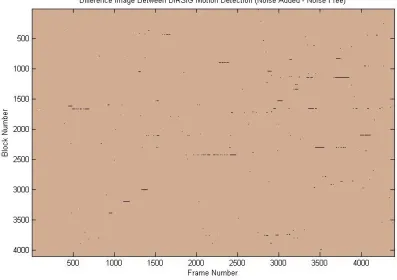
3.24 Motion Detection Difference Image: Noisy vs. Noiseless Data. 61
3.25 DIRSIG Motion Truth Frame (1024 x 1024). 62
3.26 Motion Truth Resized to (64 x 64) Block-Space 63
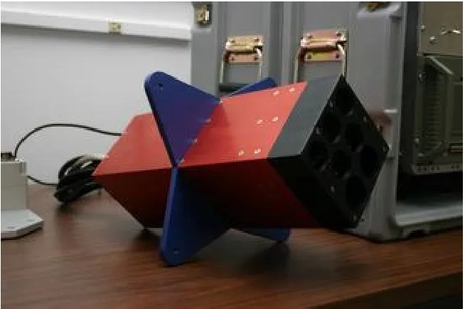
3.27 WASP Sensor System. 64
3.28 WASPLITE Imaging System. 65
3.29 WASPLITE Sensors. 66
3.30 Instrument Setup (WASPLITE Data Collection). 67
3.31 Example Frame (WASPLITE Collection). 68
3.32 WASPLITE Image Registration (RGB; 3-Band Example). 69
3.33 Original Image (Top) vs. Background Model (Bottom). 71
3.34 Motion Truth after Processing. 72
3.35 Motion-matrix Comparison (Left - Truth, Right - Detected). 74
3.36 Motion-matrix Difference (Truth Detected). 75
3.37 False Alarms, Missed Detections, and Motion Truth vs. Frame. 76
3.38 Performance Surfaces: False Alarms, Missed Detections. 76
3.39 Overlap of Truth and Detected Objects (WASPLITE Example). 77
3.40 Matlab Code for Object Segmentation Metrics. 78
3.41 Performance Surfaces: False Objects, Missed Objects. 78
3.42 Histograms of Separability Vector (WASPLITE Example). 79
3.43 Normalized Histograms of Separability Vector (WASPLITE Example). 80
4.1 System Flow Diagram (Input Data Filter). 84
4.2 Notional Missed Detection Results. 85
4.3 DIRSIG Principle Component Analysis. 86
4.4 WASPLITE Principle Component Analysis. 87
4.5 Motion Measure for Large/Slow Moving Object. 88
4.6 Motion Measure for Small/Fast Moving Object. 88
4.7 Motion Detection Ghosting (Seven-Frame Temporal Window). 89
4.8 False Alarms (DIRSIG Example). 91
4.9 Missed Detection (DIRSIG Example). 92
4.10 False Alarms (WASPLITE Example). 94
4.11 Missed Detections (WASPLITE Example). 95
4.12 DIRSIG Motion Detection Results. 97
4.13 DIRSIG Motion Detection Results. 98
4.14 DIRSIG Object Segmentation Results. 100
4.15 DIRSIG Object Segmentation Results. 101
4.16 WASPLITE Motion Detection Results. 103
4.17 WASPLITE Motion Detection Results. 104
4.18 WASPLITE Object Segmentation Results. 106
4.19 WASPLITE Object Segmentation Results. 107
4.20 WASPLITE Object Association Results. 109
4.21 Difference Vector Between Best and Next-Best Match. 110
4.22 Object Separability (Normalized). 111
4.23 Normalized Object Separability (Threshold = 0.5 σ) 112
A.1 WASP Spatial Resolution Comparison. 122
A.2 WASPLITE Spatial Resolution Comparison. 122
B.1 Second Generation DIRSIG Video. 126
C.1 Three Step Object Association Process. 128
C.2 Multiple spectral matches. 129
C.3 Convert Spectral Objects to Grayscale. 130
List of Tables
3.1 List of Segmented Object Attributes. 47
3.2 Order of Increasing Spectral Resolution. 53
3.3 Variable Frame Rates (DIRSIG vs. WASPLITE). 55
3.4 WASPLITE Camera Filters. 66
Chapter 1
Introduction
The challenge of persistent surveillance has become increasingly important in terms of national security in light of world events over the last few years. The notion of persistent surveillance is wide reaching and multifaceted with several different interpretations. The Department of Defense defines the term as “…the ability of collection systems to linger on demand in an area to detect, locate, characterize, identify, track, [and] target…to deter or forestall anticipated adversary courses of action” [DOD:2006] Another, possibly more useful definition of persistent surveillance emphasizes “sensing suites that tailor their observations to the adversary’s rate of activity.” [Signal:2002] The goal for any successful surveillance system to achieve persistence is to track everything that moves, all of the time, over the entire area of interest.
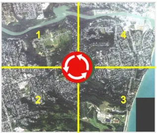
The thrust of this thesis is to identify and improve upon the motion detection and object association aspect of this challenge by adding spectral information to the equation. In order to tackle this problem, it is helpful to break it into a workable subset of challenges. First of all, consider a large geographic area of responsibility (AOR) for which a commander has the task of monitoring all activity, as depicted in figure 1.1.
FIGURE 1.1 –Area of Responsibility (AOR).
[image:16.612.148.465.391.659.2]The challenge then becomes one of achieving the same detection and tracking performance at a reduced frame rate (in this example, about 7 fps over four separate areas). Based on the simple premise that adding spectral information to the data collection should enhance detection and tracking performance, a multispectral sensor might be able to achieve the required performance at a reduced frame rate. In order to investigate this premise, we need to take a closer look at the detection and tracking tasks.
The system model of a typical surveillance system, as depicted in figure 1.3, shows three top-level tasks as moving object detection, object segmentation, and object association. In order to detect a moving object, some means of determining changes between data frames is needed. Regardless of the technique, non-moving (background) pixels are distinguished from moving (foreground) pixels. Groups of moving pixels can then be segmented into objects based on their common characteristics, such as appearance, velocity, and location. Finally, in order to establish a track, each segmented object needs to be associated to an object in the next frame.
Once a moving object has been associated from one frame to the next, second-level tasks can be performed. Depending on the objectives of the system, tasks such as track management, object classification, and behavior analysis are accomplished. Finally, these analyses can be followed by a third-level automated output or response, such as calling in further sensor assets or adjusting the current sensor allocation to a sub-region of heightened interest. The focus of this thesis is in the top-level tasks of moving object detection, segmentation, and association (as identified by the green components in the system diagram in figure 1.3).
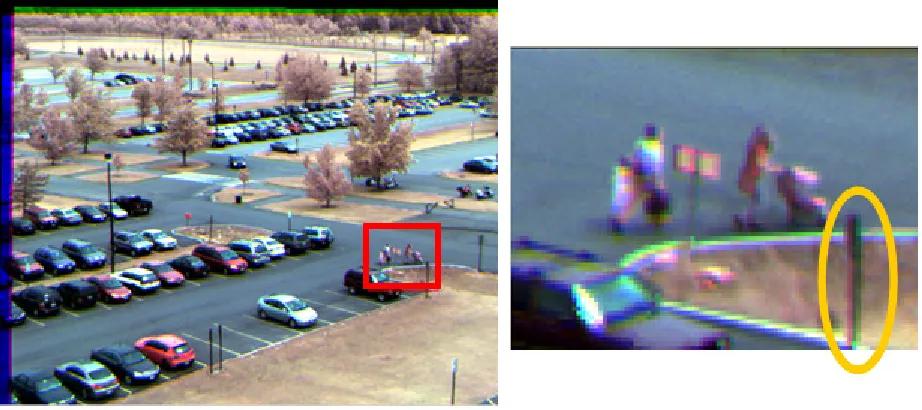
The premise of adding spectral information to current single-band techniques has merit, making improved performance at reduced frame rates seem plausible. In each of the three tasks identified (detection, segmentation, and association), additional spectral content provides useful information. First, in the case of moving object (or change) detection, typical single-band systems rely on a single grayscale value per pixel to decide if something has changed from one frame to the next. By adding additional bands of information to each pixel, change detection becomes more sensitive to subtle changes and more discriminating to non-important changes.
The simplest example is an area of pixels in one frame which may have the same grayscale appearance as in the next frame, but in reality a person wearing a red sweater is crossing in front of a red-brick building. Such a change might be missed using a single-band (or even color) sensor. However, given an additional thermal band, the bright (hot) person would stand out from the dark (cold) building.
Once moving pixels are identified, object segmentation in a single-band system relies primarily on pixel location, or proximity, to group pixels into an object. Additional information such as common velocity or appearance might help to distinguish if two objects have come together, or even if one object is temporarily obscuring the other. However, at reduced frame rates, the position and velocity estimates become unreliable. Again, by adding spectral detail to the appearance model of each object, distinguishing two or more objects becomes easier. Finally, object association in a single-band system typically becomes a task of spatial comparison of brightness value distributions and object characteristics such as velocity. Even the simplest spectral techniques such as spectral angle mapping (SAM) could provide a significant advantage over single-band techniques in object discrimination. In this case, instead of modifying existing single-band techniques to include spectral data, we can apply an additional filtering step such that we can compare objects spectrally first and then spatially.
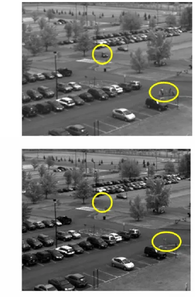
(a) Single-band at 30fps
(b)Single-band at low fps
FIGURE 1.4– Moving object ambiguity (grayscale).
However, by adding spectral detail to each object (color in this simple example), as seen in figure 1.5, the ambiguity is resolved and the two objects can be distinguished.
Current research has not emphasized this particular aspect of persistent surveillance, presenting an opportunity for novel work. An exhaustive review of current motion detection and tracking research shows two related areas of interest: multi-sensor fusion (particularly in visible/IR) and low frame rate, visible-band tracking. However, there doesn’t appear to be any current research in the combination of the two ideas: Using multispectral data to enable low frame rate methods.
Based on the above discussion, the objective of this research was to evaluate the impact of including spectral information in current motion detection and object association algorithmswith specific emphasis on reduced frame rates. Two different video datasets were used: one synthetic and the other real world data. The synthetic dataset was developed for this project by using Digital Imaging and Remote Sensing Image Generation (DIRSIG). The real world dataset was collected using the WASPLITE system; a portable version of the Wildfire Airborne Sensor Program (WASP) sensor platform. Measures of performance as a function of spectral and temporal resolution were also developed. The trade study was successfully assembled to evaluate the potential advantages to be gained by replacing current single-band video surveillance systems with multispectral sensors.
Chapter 2
Background
A review of existing methods for moving object detection and tracking provides a framework for determining the methodology for this research. Algorithm selection was based on three criteria: First, to find the most recent, “state of the art” techniques; Second, to determine which techniques would adapt well to multispectral data; Third, to allow for low frame rate input data. The background section is organized into three general areas of interest: moving object detection; object association and tracking; and current research in visible/IR fusion and low frame rate tracking methods.
2.1 Moving Object Detection
When considering the detection of moving objects in a scene an important distinction must be made based on the time interval between observations. The earliest work in processing multiple collections of the same scene occurred prior to the appearance of video surveillance. The distinction between change detection and motion detection stems from their different objectives. Whereas change detection techniques attempt to determine large scale changes in a scene over large time intervals, motion detection methods operate on a very small time scale and attempt to estimate the position and velocity of moving objects.
2.1.1 Change Detection
primarily on image differencing and required the images to be co-registered. These techniques were based on statistical measures of similarity between images [Kawamura:1971] and segmentation by region matching using features such as size, shape, spatial and even spectral properties [Price:1977]. Other multi-temporal techniques used temporal trend analysis [Engvall :1977] and Principal Component Analysis [Byrne:1980], both of which were applied to Landsat data. As change detection techniques evolved, more sophisticated approaches to image differencing techniques emerged. Variations on determining an appropriate change threshold led to measuring the change in other image quantities such as the entropy of the histogram [Kapur:1985] and intensity gradients [Parker:1991]. Difficulties in detecting change in remotely-sensed images can arise from misregistration [Townsend:1992] [Bruzzone:1997], or drastic changes in lighting, atmosphere, and sensor calibration between the two acquisition dates [Singh:1989].
More recent work has continued to improve unsupervised change detection by applying a simple yet adaptive decision threshold [Bruzzone:2002], using the assumption that the histogram of the difference image can be modeled as a mixture density of two classes: changed and unchanged pixels. The difference image (XD) is defined as the magnitude of the spectral change vector, computed for pixel (i, j) as shown in equation 2.1, where X1 and X2 are vectors of brightness values at selected bands,
XD (i, j) = || X1 (i, j) – X2 (i, j) || . (2.1)
This technique was applied to data collected by a passive multispectral scanner installed on a satellite (Wide Field Sensor (WiFS) on the IRS-P3 satellite, where X1 and X2 are multi-temporal samples of the same location on two captured images. A large value for XD indicates a changed pixel, whereas a small value is an unchanged pixel. In this way, XD is modeled as a mixture density of changed or unchanged pixels. The method is adaptive in that it does not assume an a priori model of the data distribution and semiparametric because Bayesian decision theory is used to determine the correct mixture.
Of particular interest in this example, the process uses change vector analysis (CVA) to generate the difference image. In this case, each pixel in the image is represented by a spectral vector and each pair or corresponding pixels in the two images produces a “spectral change vector”. Using the magnitude of the change vector at each pixel, the resulting spectral change map produces a grayscale image where higher values indicate greater change. Spectral change mapping will be considered further in the methodology section of this thesis.
The technique does not derive patterns of change directly from the observed brightness values. Instead, adaptive techniques use information over larger areas in a sliding window to model and predict one image from another, using what is called forward/backward prediction. In this way, subsequent observations of the same location can be put in the same frame of reference as the original observation. Thus, the difference between the original and predicted images is used as a measure of change. However, techniques such as this are attempting to resolve the change in conditions between acquisitions when the time interval is significantly greater than video surveillance frame rates. Motion detection methods applied to video are an evolution from change detection, whereby at video frame rates the scene and sensor conditions have not changed significantly between frames.
2.1.2 Motion Detection
A distinction can be made between change detection and motion detection based on the period of time between images. In modern video surveillance the standard frame rate of 30 frames per second (fps) provides a very accurate model of the scene over multiple frames. In this case we have the benefit of little environmental change between observations. Additionally, because of the short time between observations, the majority of change between frames can be interpreted as motion. Similar to change detection, the discriminating factor is in detecting moving and non-moving pixels, which can be considered as foreground (or target) and background, respectively. Similar to the distinction made in the previous section [Bruzzone:2002], the problem becomes a two-class system: moving and non-moving pixels.
2.1.2.1 Fundamental Techniques
As reviewed in the DARPA Video Surveillance and Monitoring (VSAM) report [Collins:2000], there are essentially three basic approaches to motion detection: temporal differencing [Anderson:1985]; background subtraction [Haritaoglu:1998] [Wren:1997]; and optical flow [Lucas_Kanade:1981] [Barron:1994]. Although temporal differencing is straightforward and is adaptive to dynamic environments, it doesn’t always extract all relevant feature pixels. Conversely, background subtraction generally provides complete feature data but is adversely sensitive to dynamic scene changes such as variation in lighting. Furthermore, background subtraction requires training observations in order to build up a background model. Optical flow is essentially a motion estimation technique useful in that it can detect moving objects in the presence of camera motion; however, it is computationally expensive, assumes constant velocity, and requires a suitable threshold to discriminate moving objects. Of the three fundamental motion detection methods, background subtraction appears to be the most widely used due to its simplicity and robustness [Porikli:2005].
2.1.2.2 Motion Salience
from “motion clutter” [Collins:2000] resulting from distractions such as objects blowing in the wind, moving shadows, or sensor noise. Salience of moving objects can be used for filtering out distracting, unimportant motion. Salient motion can be defined by objects with directionally consistent motion such that only objects moving “with a purpose” are detected [Wixson:2000]. Therefore, a surveillance system should also rely on motion salience for false alarm rejection. Although this technique was not applied in the methodology for this trade study, it is a point of interest for future versions. As a graduate-course project, motion salience was applied to grayscale video data to determine the feasibility of implementing such a filter [Adams:2006].
A simplified method to determine if objects are directionally consistent applies optical flow to the difference images as opposed to the original frames [Tian:2005]. The algorithm employs a temporal filter on the pre-processed scene to determine the flow field properties over time (typically 10 frames). The filtered scene then highlights only the salient objects, ignoring the non-interesting motion.
FIGURE 2.1 – Salient Motion Mask Removes Distracting Motion [Adams:2006].
the temporal filter which determines which pixels had a consistent motion over a period of 10 frames. Finally, the upper right corner (d) shows the masked scene with only the running figure isolated from the rest of the distracting motion.
2.1.2.3 Hybrid Techniques
The most recent strategies in motion detection apply a hybrid approach to the three fundamental techniques. The VSAM system [Collins:2000] employs frame differencing and adaptive background subtraction with some success, by first detecting motion using three-frame differencing then extracting region information based on an adaptive background model. Motion detection is then accomplished in a layered approach by first conducting a pixel analysis to determine moving pixels, followed by a region analysis to decide if a detected object is still moving or temporarily stationary. Another very interesting hybrid approach employs a threshold to spatiotemporal entropy [Jing:2004], where each pixel is described by the entropy of an accumulated histogram of brightness values in a local window (spatial) over several frames (temporal). However, spatial structure (i.e. edge pixels) affects the histogram adversely. The hybrid solution was to accumulate the histogram from the difference image between consecutive frames. Although the detection results were promising, the approach was overly complicated, computationally expensive, and still sensitive to illumination changes. Furthermore, this technique did not appear to be easily extended to multispectral data.
2.1.3 Spatiotemporal Texture Vectors
There is another such hybrid strategy which observes local variability in a spatiotemporal sense, also detecting motion where spatiotemporal variability exceeds a local threshold. In this other approach, the spatiotemporal description of each pixel is cast into a local “texture vector” and simplified using principal component analysis. Because of this inherent step to reduce dimensionality, spatiotemporal texture vectors appear to be an ideal choice for extending the technique to multispectral data.
The novel concept of using spatiotemporal texture vectors [Latecki_Miezianko:2006] to detect local variability in space and time seems promising. Of the three fundamental techniques listed in section [2.1.2.1], this method most closely resembles background subtraction in that it requires training observations (assuming no motion) to develop a model of background behavior. However, it has been shown to outperform the most popular background subtraction technique which uses a Gaussian mixture model to model the background [Stauffer_Grimson:1999].
FIGURE 2.2 – Spatiotemporal Texture at a Single Block.
The dimensionality of each SP-vector can then be reduced by applying principal component analysis using a 192 x 192 covariance matrix. The covariance matrix is estimated based on multiple observations of the same two dimensional region of the scene over an initialization period. Consequently, each 8 x 8 spatial window at a given time (t0 in figure 2.2) is represented
by a 10-element vector by keeping only the first ten principal components.
Motion detection is then achieved by applying a dynamic threshold to local variation in spatiotemporal texture space, tagging all the pixels in the 8 x 8 window as moving if the local behavior is inconsistent with the background model. As with traditional background subtraction techniques, this approach relies on an initialization period assuming no motion in the scene to establish the background model. Once the detector is running on an active scene, the background model is updated only when a pixel is determined to be stationary.
FIGURE 2.3 – Motion Orbits Demonstrate Spatiotemporal Variability [Miezanko:2006].
The most attractive aspect of this technique is the data structure is inherently able to include multiple spectral bands simply by extending the length of the SP-vectors. Given a motion detection technique that can be applied to multispectral data, the next task is segmenting the moving pixels into moving objects. Once all moving objects have been identified in each frame, the critical task in tracking them is to make an association between objects from one frame to the next—a task which should also be made easier given the advantage of multispectral data to discriminate between different objects.
2.2 Object Segmentation
In order to perform the next step of associating detected objects from one frame to the next, object segmentation is a necessary processing step. Once all pixels (or square regions) of a frame are labeled as moving or not moving, the moving pixels can be grouped into contiguous objects based on proximity, connectivity, and appearance. Although there is a tremendous amount of literature focused on this specific topic, it was not considered a primary area of research for this project. A more detailed description of the segmentation scheme is provided in the methodology section.
2.3 Object Association and Tracking
are matched from one frame to the next [Hu:2004 – Survey]. Also called object association, there are four major categories of methods for matching objects: model-based, contour-based, feature-based, and region-based. Any combination of these four methods can be considered a fifth, catch-all means of matching objects, such as using both regional variations in the image and specific object features [Cavallaro:2005].
Once objects have been matched from one frame to the next, track management consists of track-labeling tasks such as track initiation, splitting, merging, updating, and termination. In this trade study, track management is considered a second level function (as depicted in the system diagram in figure 1.3). As such, an overview of track management approaches will be presented, with the intention of selecting a suitable method to track multiple moving objects. The emphasis, however, is on object association, as it stands to show the greatest improvement by adding spectral information to object descriptions. Furthermore, when considering low frame rate data, motion models tend to fail due to the dynamic nature of the moving objects. In this case, we rely even more heavily on the spectral appearance model of the objects to assist in object association rather than the uncertain predictions of location and velocity.
2.3.1 Object Association Methods
The most crucial step in tracking a moving object is deciding which track it belongs to—also called object association. As reviewed by [Cavallaro:2005] and [Hu:2004], there are four basic methods for performing the object association task. The first method, model-based matching, requires a priori knowledge of object shape. Although it handles partially occluded objects based on the fidelity of the model, it is computationally expensive and is limited to the database of objects [Koller:1993]. The second method, contour-based matching, tracks only region boundaries by using “snakes” or meshes that allow for deformable objects. However, because the technique requires a complete contour, it is unable to track partial occlusions [Peterfreund:1998][Gnsel:1998]. The third method, feature-based matching uses spatial features such as edges, line segments, or corners to uniquely match objects. Although tracking a portion or subset of an object allows for partial occlusions, grouping by features makes object identification difficult [Beymer:1997]. The fourth method, appearance-based matching, uses object characteristics such as color and texture. Appearance-based methods are similar to the feature-based methods because they both rely on neighboring pixels and fail to track complex deformations [Meier:1998][Tao:2002]. However, appearance-based matching uses spectral information within the region as well as spatial, which makes it the most attractive technique for processing multispectral data.
in the next frame. Essentially, the displacement d of a target is estimated by accumulating a weighted sum of absolute intensity differences between a region in the previous (target) frame and a region in the current (candidate) frame. The best position match is given by the displacement dˆ that minimizes the correlation. This technique will be discussed in greater detail
in the methodology section.
A fifth category of object matching techniques can be derived as a hybrid of any of the four above techniques. One example of a hybrid presented by [Cavallaro:2005] proposed a hierarchical approach where the object features were first used for initial object segmentation. Next, region appearance values such as color, texture, and optical flow were used to describe the local area surrounding each object. In this case, each region was represented by region descriptors which were finally used for data association and track labeling. This example provides good insight to a future direction in hybrid object association and tracking methods— one which will emphasize local spatiotemporal variability combined with spectral matching. In fact, as described in the future work section, a proposed method combines these ideas into a three-step process (see appendix A). The first step compares the spectral similarity of objects, assigning a score. The second step converts the multispectral data into an optimized grayscale map based on distance to the spectral mean. The third step compares the grayscale objects in the VSAM single-band method mentioned above. As a result, the combined spectral and spatial similarity scores should provide a higher fidelity matching scheme than current techniques.
2.3.2 Spectral Matching
With the intention of using spectral information as the first step in object matching, we can expand the appearance-based methods to include spectral target detection techniques. Even the simplest techniques such as Spectral Angle Mapping (SAM) [Yuhas:1992] should produce additional information for matching not accounted for in the single-band methods. SAM compares two pixels by computing a spectral angle between each spectrum, as shown in equation 2.2, where x and y are two multidimensional spectra,
. (2.2)
FIGURE 2.4 - The Spectral Angle Mapper (SAM) [Shippert:2006].
Depending on the results of using SAM to produce initial similarity scores, it might be advantageous to apply other statistical spectral matching techniques such as root mean squared error (RMSE). One limitation of SAM is the insensitivity to magnitude—although the mean spectral vectors may line up, a significant deviation in magnitude would not be detected. RMSE, on the other hand, is a simple statistical measure of the band-by-band deviation of each mean candidate spectra as compared to the mean target spectra, as seen in equation 2.3 [Taylor:1997],
∑
=−
=
int
ic
in
RMSE
1
2
)
(
1
. (2.3)
In the above equation, ti is the i
th
band of the target mean spectrum and ci is the i
th
band of the candidate mean spectrum. Each candidate would be measured against the mean spectrum of the current target.
2.3.3 Track Management
Once the object association (or object matching) task has been accomplished, the surveillance system must decide how to label each object—whether it belongs to an existing track or becomes a new track. Although a full-blown tracking system is was not developed for this project, it is essential to understand the basic elements of a tracking system and how they relate to the detection, segmentation, and object association sub-tasks.
Many tracking systems are based on Kalman filters in order to predict the state of an object in the next frame. However, Kalman filter approaches are limited because they assume a unimodal Gaussian density that cannot support multiple motion hypotheses [Collins:2000]. The Kalman filter is also limited in some applications where a nonlinear motion model is required. The so-called Extended Kalman Filter (EKF) is an extension of the linear Kalman filter, applicable to nonlinear measurements and/or nonlinear target dynamics [Blackman:1999]. Multiple Hypothesis Trackers (MHT) were introduced by [Reid:1979] to form and manage multiple hypotheses whenever there are observation-to-track conflicts. It consists of a deferred decision logic in which alternative data association hypotheses are formed in anticipation that subsequent observations will resolve the conflict [Blackman:1999].
Another approach to Kalman filtering and MHT—as developed in the VSAM system for DARPA [Collins:2000]—is to maintain a list of multiple hypotheses to handle cases where object matching between multiple objects is ambiguous. The method assumes there are five tracking scenarios: 1) A new object appears; 2) An existing object disappears; 3) An object matches exactly one track; 4) A single track splits into multiple objects; or 5) Multiple objects merge into a single track. In this tracking system, object trajectories are also analyzed to reduce false alarms by evaluating object persistence and motion salience. The VSAM tracking method was determined to be suitable for this research, the details of which are covered in the methodology section.
The VSAM tracking system further divides the tasks into the following steps, which are covered in the following subsections:
• Predict positions of known objects
• Associate predicted objects with current objects
• Hypothesis Tracking
• Update object track models
• Reject false alarms
2.3.3.1 Predict Positions
The first step, predicting the location of objects in each frame, requires an estimate and uncertainty of the future position of each object being tracked. Given the time between frames
∆
t, the estimated position is simply based on the expected displacement due to the previous velocity estimate (assuming constant acceleration), as shown in equation 2.4 [Collins:2000],. (2.4)
Thus, the uncertainty in the position is based on the uncertainty in the velocity estimate used, as shown in equation 2.5 [Collins:2000],
. (2.5)
The estimated position is used to choose candidate moving regions in the current frame by extrapolating the previous location. The future position is then assumed to be somewhere between the previous location and a reasonable location within the bounds of what is physically possible. Keeping low frame rates in mind, thus considering a significant increment of time between frames, the object could conceivably change or even reverse direction. Thus, a ring based upon a maximum velocity is drawn around the previous location, with the most likely location being along the previous course. Any candidate object that falls within this ring will be considered for matching, with greater confidence given to a match on the expected course.
2.3.3.2 Associate Predicted Objects
Various object association techniques were discussed previously in section [2.3.1]. Because the focus of this research is to enhance existing methods by including spectral information, the tracking process described thus far is suitable for track management. However, the key concept of enhancing the object association step using spectral information is described in greater detail in the methodology section.
2.3.3.3 Hypothesis Tracking
1) Existing track matches exactly one candidate – Best case
2) Existing track does not match any candidates – Stopped or lost
3) Existing track matches multiple candidates – Split
4) Candidate matches multiple existing tracks – Merge or Occlusion
5) Candidate does not match any existing tracks – New track
In the first case, where the existing object matches exactly one candidate, the update is simple. The state parameters (position, velocity, etc) are updated based on the matched object and the confidence score is increased. The second case—in which the object has stopped, been occluded, or left the scene—requires more information. Thus, the state parameters remain unchanged aside from a reduced confidence score until a future match is made. If the confidence score falls below an empirical threshold, the object track is terminated. The third case, where multiple candidates are reasonably close matches, can result from an object splitting into several objects, either in reality (such as passengers dismounting a vehicle) or due to a failure in the detection algorithm to properly cluster all the moving pixels into one object. In this case, the best match is assigned to the existing track with increased confidence. The remaining matches are considered new tracks with associated low confidence, pending further information. The fourth case is the alternative to the third case, where one candidate matches multiple existing tracks reasonably well. In this case, multiple moving objects have actually merged into one (such as passengers mounting a vehicle), are traveling near or are occluding one another, or the anomalous detection of multiple objects has been rectified. Further information is again required to determine what is actually happening. In this special case, the objects are tracked separately under the assumption they are most likely sharing the same region but not actually merged. Each existing track is updated using the same matching candidate object. If the multiple tracks continue along the same trajectory with the same velocity for a period of time they can be merged. Otherwise, they are tracked separately under the assumption they will split again in future observations. In the fifth and final case, a new object is hypothesized with low confidence pending further matches.
It is instructive to note that at the beginning of a tracking session—when no matches or tracks have yet been established—all detected moving objects are hypothesized as new tracks with low confidence and are equally likely to head in any direction. It is here, once again, that adding spectral information could provide an advantage over the traditional single-band tracker. With no position or velocity estimates, the matching process is weighted more heavily on spectral similarity. In comparing spatial confidence with spectral confidence, it is important to note that spectral confidence should increase with the number of bands (assuming the spectral bands are sufficiently uncorrelated). Conversely, spatial confidence should decrease with decreasing frame rate, because the uncertainty in the predicted location goes up as the time increment between frames increases.
2.3.3.4 Update Tracks
(displacement divided by
∆
t) and the previous velocity vn, as shown in equation 2.6[Collins:2000],
, (2.6)
where α is a time constant specifying how frequently old observations are updated. Likewise, the velocity uncertainty is updated as shown in equation 2.7 [Collins:2000],
. (2.7)
The spectral and grayscale templates of the object are updated in similar fashion using a running average (or median). However, in the case of multiple tracks being matched to a single candidate region (merge), the templates are not updated in order to preserve the previous individual appearance of the tracked objects. Again, this applies the assumption that the most likely scenario is objects traveling near one another that will eventually split again. Any track that has not been matched will not be updated except for a reduced confidence score. An object that has been tracked for several frames will have a relatively high confidence. In the event that an object temporarily stops or is occluded in motion, the track will persist for a number of frames before it is terminated. As such, a high confidence track will have a likelihood of being reacquired in a later frame.
2.3.3.5 Reject False Alarms
Possibly the most troublesome aspect of any detection and tracking system is the problem of false alarms. In order to validate a moving object as a legitimate target, a history must be established. There are two attributes that can validate such a target: persistence and motion salience. The persistence of an object is handled by the tracker in the form of an updated confidence score. Once an object falls below a confidence threshold the track is terminated. Thus, a newly detected object is given a low confidence and will remain above the threshold only if immediate updates increase the confidence. In contrast to new tracks, existing tracks with sufficient history will be allowed to persist longer without a match in anticipation of reacquisition of a valid object.
when propagated over several frames [Adams:2006]. A short cut method [Collins:2000] provides a means to compute motion salience based on three parameters, which are initially set to zero: frame count c, cumulative flow dsum and maximum flow dmax. For each frame, the
displacement of each object is accumulated into dsum and the frame count is incremented. If accumulated flow dsum is greater than dmax, it is reassigned as the new maximum. If dsum falls
below 90% of the maximum flow dmax, it is assumed that the direction of the object has reversed
and all parameters are set back to zero. The calculations are performed in both the x- and y- image direction in such a way that objects maintaining an accumulated displacement in either direction are considered salient, and thus valid targets.
In summary, the example tracking system described above will predict object locations, associate objects, manage multiple hypotheses, update valid tracks, and reject false alarms. However, this is simply one technique among numerous other tracking systems. For the purposes of this trade study, any such tracking system would be customized to meet user requirements. An essential step in modifying the tracking process is to enhance the object association step by taking advantage of spectral information. Once all moving objects are detected and associated, track management provides the time history and predicted state of each object. However, up to this point all detection and tracking techniques discussed were developed primarily for single-band video at 30 fps. Current research has branched into multi-sensor fusion (applicable to multispectral data) and tracking at lower frame rates.
2.4 Current Research
Two active areas of research that are pertinent to this trade study are visible/IR data fusion and low frame rate tracking systems. In either case, the research goal is to enhance motion detection and tracking performance. However, the two ideas are being looked at independently, without the intention of using data-fusion to enable low frame rate tracking. Research regarding fusion of visible and IR sensors has primarily been with the goal of either enhancing daylight surveillance or enabling nighttime surveillance. On the other hand, low frame rate tracking techniques have the exclusive goal of reducing collection bandwidth and/or enabling surveillance with very low cost equipment. An exhaustive review of the most current tracking technology shows very few people are approaching the problem in a multispectral sense. Up to now, the notion that multispectral data might enhance low frame rate tracking performance is apparently a unique one.
2.4.1 Visible/IR Fusion
with a per-pixel importance weighting to track image regions. The study concludes that the most promising combination of individual trackers results from a simple multiplication of the similarity scores, called the similarity score product. Of particular interest, this study models the appearance of the object being tracked as a rectangular grid of d pixels, with each pixel being modeled by a Gaussian distribution. In this way, each pixel at a given time t can be represented by the mean vector of k values, where k is the number of features. Assuming pixel features are independent, the model also includes the diagonal covariance matrix to characterize each pixel. Such an arrangement is particularly attractive when considering the problem as a multispectral one, where each pixel is, in fact, k-dimensional. Finally, they include a weighting factor to each pixel that will remove background pixels from the object region while emphasizing valid features.
The above fusion approach is extended to track objects by using multiple spatiograms trackers [O'Conaire_2:2006]. In this way, the system can process K different channels of data by
comparing K one-dimensional histograms. However, in the case of histograms the assumption of
independence does not hold. The problem is resolved by introducing second-order spatiograms, which include spatial information by weighting each histogram bin by the mean and covariance of the pixel locations that contribute to that bin [Birchfield:2005 – Spatiograms versus histograms]. As a result, the technique successfully incorporates the results from each single-band tracker by using the combined product of the individual spatiogram similarity scores, as shown in equation 2.8,
Combined Similarity:
ρ
(y) =ρ
(1)(y)ρ
(2)(y)... ρ
(Κ)(y). (2.8)The technique of multiplying individual similarity scores for each separate spectral band to achieve a combined score is intuitive when considering each similarity score as an individual probability.
However, as will be explained in detail in the methodology section, it is more straightforward to match objects by first using a spectral similarity measure, followed by a single-band similarity score rather than combining K separate trackers. After a spectral comparison, the spectra could be reduced to a grayscale and then compared spatially. This is of particular concern when considering low frame rate data where significant time may have passed between frames. In this case, the spectral similarity might be more reliable and therefore weighted more heavily than the less certain spatial qualities of the target. Tracking objects at low frame rates has other potential pitfalls, as described in the next section.
2.4.2 Low Frame Rates
such as people and vehicles remain spectrally constant—a yellow school bus is still yellow and people and vehicles remain relatively the same temperature. Now the challenge becomes handling changes in motion, such as abrupt changes in direction and velocity that were not a problem at 30 fps. Another way of looking at the problem is to compare low frame rates to increased object velocity (or frame-to-frame displacement). In this case we can see that motion models will fail as uncertainty between observations increases. Successful matching then relies upon the spectral signature of targets remaining constant enough to find and associate every moving object from one frame to the next.
The most current work (in a notably sparse area of research), approaches low frame rate tracking as a means to improve processing time and to reduce bandwidth and storage limits [Porikli:2005]. The paper shows the anticipated degradation in tracking performance as a function of reduced frame rate, as seen in figure 2.5. A system tracking a single object tended to suffer the least degradation, while tracking multiple objects suffered the most due to object ambiguity.
FIGURE 2.5 – Object Tracking Accuracy as a function of frame rate [Porikli:2005].
it does not attempt to add spectral information to help determine the otherwise ambiguous location of objects in the next frame. The technique of attempting to associate targets with all candidates—regardless of location—will be addressed in the methodology section.
Considerable progress is being made in both data fusion and low frame rate trackers. However, the intention of this project was not necessarily to solve either of these problems independently. Rather, it is to investigate trades in performance as a function of the number of spectral bands and frame rates simultaneously. As such, performance metrics for moving object detection and association are needed to compare results using different settings within this trade space.
2.5 Performance Metrics
As presented by [Bashir:2006], there are two basic methods to evaluate tracking system performance by using either frame based or object based metrics. To achieve an overall perspective of the trade space for this project, the performance metrics derived for this study were somewhat less complex. However, frame- and object-based metrics are included in this section for future consideration when evaluating a complete tracking system. In addition, the perceptual complexity of a scene can be useful when evaluating the performance of a system [Black:2003].
2.5.1 Frame Based Metrics
In frame based metrics, each frame is evaluated individually for agreement between system results and the ground truth (GT) map for that frame. In this case, when comparing a system frame to the ground truth frame, two object bounding boxes are “coincident” if one centroid lies within the other box. Once each frame is evaluated, there are a number of metrics that can be considered by computing the total number of frames that meet each of the following criteria [Black:2003]:
• True Negative (TN): System agrees with GT on absence of an object
• True Positive (TP): System agrees with GT on presence of an object
• False Negative (FN): System does not report object when GT does
• False Positive (FP): System reports object when GT does not
• Total Ground Truth (TG): Total number of frames with ground truth objects
• Total Frames (TF): Total number of frames in video sequence
(2.9-2.11)
The tracker detection rate (TRDR) and false alarm rate (FAR) characterize the tracking performance of the object-matching algorithm, while the detection rate (DR) indicates the tracking completeness of a specific ground truth track. As an example of how these metrics can be used to compare tracking systems, figure 2.6 shows TRDR and FAR results for six different tracker/detector combinations [Black:2003]. A similar comparison could be made between a system using a variable number of bands and/or variable frame rates.
Other more specific metrics, as presented by [Bashir:2006], can be generated as shown in equations 2.12 through 2.17:
(2.12-2.17)
The above metrics are based upon counting the number of frames that either agree or do not agree with the ground truth frames and then considering the desired ratio to the total number of relevant frames in the video sequence.
2.5.2 Object Based Metrics
FIGURE 2.7 - Object Correspondence Map [Bashir:2006].
Once a correspondence is established, the true positive (TP), false positive (FP), and total ground truth (GT) are computed as explained in the frame-based method. The tracker detection rate (TRDR) and false alarm rate (FAR) are likewise computed similar to frame based methods.
Finally, a single-value called the object tracking error (OTE) can be computed as the average discrepancy between the GT bounding box centroid and the system result centroid, as shown in equation 2.18,
OTE
=
. (2.18)
In this computation, Nrg is the total number of overlapping frames between ground truth and
system results over the entire video sequence. Ground truth coordinates (xig, yig) and system
result coordinates (xir, yir) are the respective image locations of the object centroids, where
i-subscripts indicate the ith frame. In this way, a single performance score can be assigned to each
object tracked by the system. A combined score would simply be the combination of an OTE for
each object in the sequence. Although a single score for each tracking system configuration is useful, the combined score might be oversimplified unless the complexity of the tracking scenario is also considered.
2.5.3 Perceptual Complexity
As described by [Black:2003], the perceptual complexity of a scene can be controlled by a set of tunable parameters using “pseudo-synthetic” video sequences. The two parameters suggested
are the maximum number of objects to be tracked (MAX) and the probability of creating a new
shown in figure 2.8, where perceptual complexity (average number of objects per frame) increases with the probability of adding a new object in any given frame [Black:2003].
FIGURE 2.8 – Perceptual Complexity [Black:2003].
Although the datasets for this project did not allow for a variable probability of new objects, the synthetic video sequence was designed to have an increasing number of targets as a function of time. This allowed for a sense of perceptual complexity in that early scenes are simple and become more complex as new objects are added.
2.6 Background Summary
Chapter 3
Methodology
After reviewing the state-of-the-art in moving object detection and tracking systems, a hybrid approach was devised. The newly devised object detection and association system modified current algorithms by including spectral information with the specific goal of achieving improved performance at reduced frame rates. The system model shown in the introduction (figure 1.3) provides a framework to determine which subtasks might gain by adding spectral information, and to what degree. The emphasis was on moving object detection, segmentation, and association. Once implemented, a trade study was conducted to determine system performance as a function of spectral (number of bands) and temporal (frame rate) resolution. In order to perform such a trade study, performance metrics were needed. Both synthetic and real world datasets were generated to provide relevant results and conclusions.
In order to limit the scope and objectives of this project, some simplifying assumptions were made. The scene collection was assumed to be from a stationary platform over an urban environment; thus, parallax and platform stability issues were not addressed. With an emphasis on developing a theoretical methodology, processing power and data storage were not considered limited by any specific system requirements. Finally, all frames were assumed to be registered to less than one pixel accuracy, which was perfectly true with synthetic data.
segmentation and object matching performance under the hypothesis that improved performance in these subtasks is directly correlated to improved performance in a complete tracking system.
3.1 System Model
Starting with the model of a surveillance system, the intention of this research was to focus on potential improvements in a subset of tasks. As highlighted in figure 3.1, modifications to existing moving object detection, segmentation, and association techniques were studied. The first step was to modify single-band spatiotemporal texture vectors [Miezanko:2006] to include additional bands of data. Hence, a more sensitive detector was expected. The second step, segmentation, also gained an advantage by discriminating between background pixels and clustering spectrally similar pixels into objects. The third step, object association, measured the effective advantage of a multispectral system in matching an object from one frame to the next.
FIGURE 3.1 – System Model with subset of tasks highlighted.
3.1.1 Motion Detection Using Spatiotemporal Texture Vectors
FIGURE 3.2 – Motion Detection Flow diagram.
The accumulation of pixel values over space and time causes the SP-vectors to have high dimensionality, which is exacerbated by adding spectral bands. However, dimensionality was reduced—even in the single-band mode—by using principal component analysis (PCA). PCA projections used an estimated covariance matrix based on an initialization period where it was assumed there is little or no motion in the scene. Once the SP-vectors were reduced to a manageable size, temporal variability was monitored as compared to the initial state where no motion was assumed. A motion measure was then produced by taking the largest eigenvalue of these dimensionally-reduced SP-vectors as accumulated over a sliding temporal window. In this way, a single value was assigned to each two dimensional region, or “block” (a subspace of the entire scene), at a given time. Next, a dynamic threshold then determined if the variability in that local spatiotemporal region indicated motion. The motion detection results for all blocks over all image frames are captured in the motion-matrix. These five steps are described in detail in the following subsections.
3.1.1.1 Formation of Texture Vectors
The first step is to divide each image frame into a grid of two dimensional square regions (blocks), whereby each block of the entire frame is monitored individually. Although (8 x 8) blocks of pixels were used in the original paper, the author indicated that regions of (4 x 4) pixels work just as well to determine local variability. As such, smaller blocks provide better spatial resolution [Miezianko_Notes:2007]. In this case, the datasets were derived from single-band campus security video cameras. Of course, the division of frames into a particular grid is dictated by the resolution of the sensor and/or dataset. Based on the hypothesis that additional spectral texture would improve sensitivity, (2 x 2) blocks—or even individual pixels—might also be monitored. However, computational performance decreases as the size of each spatial window is reduced because more blocks per frame have to be processed in order to monitor the entire scene.
FIGURE 3.3 – Convert 3D block into SP-vector.
The example above shows an accumulation of (4 x 4) pixel blocks over 3 frames of grayscale video. The single-band setup produces SP-vectors with 48 brightness values. Now consider using a five-band system (as described in the datasets section) which produces SP-vectors with 240 elements. Keep in mind that the entire scene is divided into separate two dimensional blocks such that each SP-vector represents a single spatial subset over 3 frames. Thus, extending the spatiotemporal vector technique to multispectral data is simple and convenient. The single band SP-vectors are extended to a length, Lm as seen in equation 3.1,
Lm = (4 x 4 x 3 x d). (3.1)
The above equation uses (4 x 4) blocks over thre