Frequency-weighted controller and model order reduction methods in linear system design

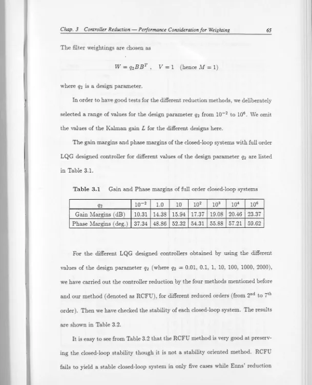
Frequency-Weighted Controller and

Model Order Reduction Methods

in Linear System Design

Yi

LIU

B.Sc. (Zhongshan Univ.)

A thesis submitted for the Degree of Doctor of Philosophy

of the Australian National University

Department of Systems Engineering

The Australian National University

1

-Declaration

Much of the work in the thesis has been published, or is being processed for publication, or under preparation for submission for publication in the relevant scientific journals. The publications are

• Y. Liu and B.D.O. Anderson, "Controller reduction via stable factorization and balancing", International Journal of Control, Vol.44, No.2, 1986, pp.507-531.

• Y. Liu and B.D.O. Anderson, "Model reduction with time delay", IEE Proc. Part D., Vol.134, o.6, 1987, pp.349-367.

• B.D.O. Anderson and Y. Liu, "Controller reduction: Concepts ana. a p-proaches", Proc. American Control Conference, Minnesota, lJSA, 1987, pp.1 -9. Also to appear in IEEE Tran3. Automatic Control.

• Y. Liu, B.D.O. Anderson and U.-L. Ly, "Coprime factorization controller reduction with Bezout identity induced frequency weightini', Automatica, accepted for publication.

• Y. Liu and B.D.O. Anderson, ''Frequency weighted controller reduction method and loop transfer recovery", A utomatica, accepted for publication. • Y. Liu and B.D.O. Anderson, "Singular perturbation approximation of

bal-anced system", submitted to International Journal of Control.

I also did some joint research work on H00-norm calculation. This work does not appear in this thesis, but is in the paper:

• L. Guo, L. Xia and Y. Liu, "Recursive algorithm for the computation of Hoo-norm of polynomials", IEEE Tran3. A utomat. Control, Vol.AC-33, No.12, 1988, pp.1154-1157.

1 1

-I hereby declare that the contents of this thesis, except as otherwise explicitly stated, are the result of original research, and have not been submitted for a degree to any other university or education institution.

Canberra, March 1989

Lt

'I

y;~(

~~

Department of Systems Engineering Research School of Physical Sciences

The Australian National University ACT 2601

- lll

-Acknowledgements

It is a great pleasure for me to acknowledge here the most invaluable guid-ance, criticisms, encouragement, and supervision of Professor Brian D.O. Anderson throughout the course of my doctoral studies at the Australian National University. The very stimulating and invigorating atmosphere of the Department of Systems Engineering has also been conducive to my interest with respect to the background and orientation of the research resulting in this thesis. Of the help given by the department, I have benefited particularly from working and discussing with Prof. J.B. Moore, Dr. R.R. Bitmead, Dr. D Williamson and Dr. L. Guo.

Thanks are also due to my fellow students for their contributions made in many informal technical discussions.

The active visitor programme at Systems Engineering has offered me the opportunity to contact many visitors, notably R.E. Skelton, U .-1. Ly, I. Postleth-waite, and M. Vidyasagar. I thank them for their inspiring discussions.

It is impossible to adequately thank Dong Feng Li, my wife, for her cont:-i-bution to my studies and life at Canberra. I am particularly grateful to her for bringing Richard, our son, to this world.

Abstract - lV

-Abstract

In this thesis, the controller reduction problem is sensibly posed as a frequency

weighted L00-norm approximation problem. The choice of frequency weighting is

influenced by the choice of criterion thought most desirable in the approximation

process.

A novel controller reduction procedure is proposed in this thesis which is

based on a representation of a controller as a matrix function defined using

sta-ble proper transfer functions in conjunction with the consideration of closed-loop

performance in choosing the weighting. For a certain right coprime factorization

of an LQG designed controller

K(s

)

=

N(s)D-

1

_(s)

_{, ·.ve approximate using a}

oal-ancing technique with a constant weighting the pair

[DT

(

s

)

JVT

(

s

)]

T

by a low order pair [

D[

(

s)

N'[

(

s)

]T

defining a factorization of the reduced order co

n-troller

K

1

(s)

=

N

1

(s)D-;

1

(s).

vVe show that this reduction procedure possesses good properties of retaining the closed-loop stability margin and closed-loop

per-formance and can handle very easily an open-loop unstable controller reduction

problem.

Based on the same fractional representation of the controller and the plant in

conjunction with a frequency weighting derived from closed-loop stability

consid-erations, this thesis presents another frequency-weighted controller reduction

pro-cedure through the use of the Bezout identity associated with the factorizations

of the plant and the controller and the frequency-weighted balanced truncation

reduction technique. It is shown that this procedure has very good properties of

preserving the closed-loop stability in the reduction. Extensions to this procedure

Abstract v

-problems or having a tradeoff between the requirements of maintaining the

closed-loop stability margin and the closed-loop performance in the reduction. Examples

are used to illustrate the above controller reduction methods.

A relationship between the Bezout identity induced frequency-weighted

con-troller reduction method and the Enns' frequency-weighted controller reduction

method is established. If a high order controller to be reduced is designed using the loop transfer recovery (LTR) technique, then the above two weighted

con-troller reduction methods are equivalent if the system is square, nonsingular and

of minimum phase. Further, if the high order stabilizing controller itself is stable

(without any LTR assumption), then the Enns' method is a special case of the

Bezout identity induced frequency-weighted controller reduction method.

For an open-loop model reduction problem, this thesis presents a procedure

for approximation of a high order system with rational transfer function together

with a pure time delay. A time delay is introduced into the system output and the

low order rational transfer function is computed using truncation of a balanced

realization. Frequency error bounds are obtained for both continuous-time and

discrete-time cases. Some examples are presented to illustrate the reductiuon

procedure.

In the thesis, the singular perturbation approximation technique for model

reduction is also related to the direct truncation technique if the system model

to be reduced is stable, minimal, and internally balanced. It shows that these

two methods constitute two fully compatible model reduction techniques for a

continuous-time system, and both methods yield a stable, minimal, and internally

balanced reduced order system with the same L00-norm error bound on the re-duction. Although the upper bound for both reductions is the same, the direct

truncation method tends to have smaller errors at high frequencies and larger

errors at low frequencies while the singular perturbation approximation method

Abstract - Vl

-only preserves the balanced structure between a continuous-time system and an

associated discrete-time system, but also preserves the slow singular perturbation

approximation structure. Hence, the continuous-time results on the singular

per-turbation approximation of balanced systems are easily extended to the

discrete-time case. Examples are used to show the compatibility and the differences of the

Table of Conterus - Vll

-Table of Contents

Declaration . . . . . . . . . . . . . . . . . . . . . . . . . . . . . . . . . . . . I Acknowledgements . . . Ill

Abstract . . . . . . . . . . . . . . . . . . . . . . . . . . . . . . . iv

Table of Contents . . . .. . . .. . .. . . .. . . vu Definitions .. . .. ... . . .. . .... .. .. . . .. . . xii

List of Abbreviations . . . .. .. . . .. . xv

Chapter 1 Introduction . . . . . ... .. . . ... . . .. . . . .. .. .. .. . 1

1.1 Why Order Reduction? . . . . . . . . . . . . . . . . . . . . . . . . . . . . . . 1

1.2 Key Issues for Indirect Methods . . . . . . . . . . . . . . . . . . . . . . . . . . 3

1.3 Related Literature . . . ... ... .. . . ... .. . . 4

~ 1.4 Contributions of the Thesis • • • • • • • • • • • • • • • • • • • • • • • • • • • • • I 1.5 Organization of the Thesis . . . . . . . . . . . . . . . . . . . . . 11

Chapter 2 Background Material . . . . ... .. .. .. .. .. . . . . 13

2.1 Introduction . . . .. . . .... . . 13

2.2 Linear Feedback System Design ... .. . ... .. . . .. ... . .. .. . . 14 2.2.1 Linear Quadratic Regulator (LQR) . . . ... ... .. . . ... 14

2.2.2 Kalman Filter . . . .. . ... .. .. . . ... .... . 15 2.2.3 Loop Transfer Recovery (LTR) . ... . . .. . .... . .. 17 2.3 Coprime Factorization Representation . . .. .. . . .. ... . . ... . . . 19

2.3.1 Definitions .. . . .. . . .. .. . . .. .. ... ... . 19

2.3.2 Coprime Factorization Representations of Plant and Compensator . . . . . . . . . . . . . . . . . . . 20

2.3.3 Graph Topology, Graph Metric and Some Related Results .. 22

[image:8.605.25.593.18.761.2]

Table of Contents

2.4.1

2.4.2

2.4.3

- Vll!

-Balanced Realization and Direct Tmncation Approximation 26

Hankel Norm Optimal Approximation . . . 29

q-Markov COVariance Equivalent Realization . . . 30

2.5 Frequency-Weighted Order Reduction Techniques . . . 32

2.5.1 Frequency-Weighted Balanced Truncation Approximation .. 32

2.5.2 Frequency-Weighted Hankel Norm Optimal Approximation . 36 2.5.3 Unstable Model Reduction . . . .. . . 37

2.5.3.1 Balanced Truncation Approach . . . 37

2.5.3.2 Additive Decomposition . . . .. . . .. ... 38

2.5.3.3 Stable Rational Fraction Approximation . . . 39

Chapter 3 Controller Reduction - Performance Consideration for Weighting . . . 41

3.1 Introduction . . . 41

3.2 Controller Reduction as a Frequency-vVeighted L00-Norm Approximation . . . .. . . ... . .. . . 42

3.2.1 Performance Considerations for Frequency vVeighting . . . 42

3.2.2 Stability Margin Considerations for Frequency Weighting 43 3.2.3 Closed-loop Transfer Function Considerations for Frequency Weighting . . . 46

3.2.4 Further Issues . . . .. . . .. ... . . ... . 47

3.2.5 Key Idea for New Controller Reduction Methods ... .. ... 49

3.3 Right Coprime Factorization (Unweighted) (RCFU) Reduction Method . . . . . . . . . . . . . . . . . . . . 50

3.3.1 Motivations for the Method . . . 50

3.3.2 Controller Reduction Algorithm ... . . 54

3.3.3 Properties of the Reduction . . . 57

3.4 Examples ... . . ... . . .. . . ... 63

Table of Conte ms - lX

-Chapter 4 Controller Reduction With Weighting

- Stability Consideration for Weighting . .... ... 80

4.1 Introduction . . . . . . . . . . . . . . . . . . . . . . . . . . . . . 80

4.2 Robust Stability Criteria and Enns' Weighted Reduction Method . 81 4.2.1 Robust Stability Criteria (for Controller) . . . ... 82

4.2.2 Enns' Frequency-Weighted Controller Reduction Method 88 4.3 Coprime Factorization Controller Reduction With Bezout Identity Induced Frequency ·weighting .. . ... . . 95

4.3.1 Left Coprime Factorization (Weighted) (LCFW) Controller Reduction Method .. . . .. .. .. .. .. 95

4.3.2 Reduction Algorithm . . . . . . . . . . . . . . . . . . . . . . . . . . . 101

4.3.3 Properties of the Reduction . . . . . . . . . . . . . . . . . . . . . . . 103

4.4 Some Extensions of the LCFvV Reduction Method .. .. ... . . 106

4.4.1 The LCFW Reduction Method for More Complex Structured Compensators .. ... . . .. 106

4.4.2 The LCFW Method With Consideration of the Closed-Loop Performance . . . 110

4.5 Examples . . . . . . . . . . . . . . . . . . . . . . . . . . . . . . . 113

4.5.1 Example 4.1 . . . .. . . .. . . .. . . 113

4.5.2 Example 4.2 . . . . . . . . . . . . . . . . . . . . . . . 118

4.5.3 Example 4.3 122 4.6 Summary ... . . ... . .. . . .. .. . ... . .. . . . 125

Chapter 5 Loop Transfer Recovery (LTR) and 5.1 5.2 5.3 Weighted Controller Reduction lVIethod . . . 127

Introduction . . . . . . . . . . . . . . . . . . . . . . . . . . . . . 127

[image:10.600.25.595.15.761.2]

Table of Contents

-x-5.4 Further Relations of the Two Methods

for Open-Loop Stable Controllers . . . . . . . . . . . . . 138

5.5 Scaling Problem for the Frequency-Weighted Controller Reduction Methods .. . .. . . .. . 140

5.6 Summary . . . . . . . . . . . . . . . . . . . . . . . . . . . . . . . . . . . 144

Chapter 6 Model Reduction With Time Delay . . . ... 146

6.1 Introduction . . . .. . . .. .. ... 146

6.2 Continuous-Time System Approximation ... . . .. ... . 148

6.3 Discrete-Time Approach .. . . .. . . .. . .. . . 152

6.4 Error Bounds . . . .. . .. . . .. ·. . . . . . . . . 154

6.4.1 Continuous-Time, SISO System . . . .. . . 155

6.4.2 6.4.3 Continuous-Time, MIMO System Discrete-Time Case 158 163 6.5 Examples . . . . . . . . . . . . . . . . . . . . . . . . . . . 164

6.5.1 Example 6.1 .. . . ... .. . . .. . .. . .. . . .. 164

6.5.2 Example 6.2 . . . . . . . . . . . . . . . . . . . . 168

6.5.3 Example 6.3 . . . . . . . . . . . . . . . . . . . . . 173

6.5.4 Example 6.4 . . . . . . . . . . . . . . . . . . . . . . . . . . . . . 177

6.6 Remarks and Summary . . . . . . . . . . . . . . . . . . . . . . . 179

Chapter 7 Singular Perturbation Approximation of Balanced Systems . . .. .... . . ... . . 187

7.1 Introduction . . . . . . . . . . . . . . . . . . . . . . . . . . . . . . . 187

7.2 Singular Perturbation Approximations (SPA) . . . ... 189

Table of Conterus - x1

-of Balanced Systems - Continuous-Time Case . . . 198

7.4 Properties of Singular Perturbation Approximation of Balanced Systems - Discrete-Time Case . . . . . . . . . . . 208

7.5 Examples .. .. . . .. ... .. ... . . ... .. ... . . .. 214

7.5.1 Example 7.1 .. . . .. ... ... 214

7.5.2 Example 7.2 . . . . .. . . 221

7.6 Summary . . . . . . . . . . . . . . . . . . . . . . . . . . . . . . . . . . 225

Chapter 8 Conclusions and Recommendations for Future Research . . . 227

8.1 Conclusions 227 8.2 Recommendations for Future Research . . . . . . . . . . . . . . . . 231

References ... . . . . . . 235

Appendix A Data of Example 4.2 . . . 245

[image:12.611.37.600.17.735.2]

Definitions _{- Xll}

-Definitions

c_

R+

A

C

Re(•)

Im(•)

J

x

X

n dimensional complex number space, C1 _{denoted as C - the}

normal complex plane.

m

x

/!_ matrix in which elements belong to C.

open left hand complex plane.

closed right hand complex plane. C+e is the extended C+, i.e.,

C+e

= {C+

plus the point at infinity}.

n dimensional real number space. R 1 _{denoted as R.}

m x /!_ matrix in which elements belong to R.

non-negative real number.

equal to, by definition.

for all.

belongs to.

AC B means: A is a subset of B.

real part of •.

imaginary part of •.

imaginary number: j 2

₌

_-1.

complex conjugate of x.

Definitions _{- Xlll}

-transpose of A ( vector or matrix).

A* A*

₌

AT

_:

comp l ex conJugate transp. ose.

GH

(s)

=

GT

(

-

s):

Hermitian conjugate transpose. When

G

(s)

has real coefficients and s is on imaginary axis, i.e., s

=

jw

, t

hen

[G(jw

)]*

=

[G(s )]H.

A-

1 _{inverse of matrix}

_A

_.

det[A] determinant of matrix A.

diag{ a1, ... , an} diagonal matrix where the ( i-i) element is ai, i

=

1, 2, ... , n.

tr{A} trace of matrix A.

rank{A} rank of matrix A.

,\i{ A} ith eigenvalue of matrix A.

o-i{A}

ith singular value of matrix

A.

Zf{A} the maximum singular value of matrix A.

£.{A} the minimum singular value of matrix A.

deg{p( s)} degreee of the polynomial

p

(

s)

.

[

•

J+

constant part and strictly proper and stable part of •.

[ • ]- non-proper and/or unstable part of•.

Definitions

JjG(jw)jjoo

Dv

- XlV

-JjX(jw)IJ~

~

J

X*(jw)X(jw) dw, if X(s)EL2_{(-oo, +oo).} -oo

Let G(s): C >--+ cmxl_ Then G(jw)EL₀₀(-oo, +oo) if and only

if there exists a real number M

<

oo such that a'" { G(j w)} ~ lvl ,

VwER.

jjG(jw)jj₀₀

~

ess supo'"{G(jw)}

=

ess supAJ'iax{G*(jw)G(jw)},

weR weR

if G(s)EL00(-oo, +oo). "ess" means essential.

Let X(

S)

:

C >--+

en.

Then X(

S

)EH2 if and only if X(

S

)

is

analytic in the open right half plane and JI X ( 17

+

j

w) j

j 2 ~ lvl

<

oo, \117

2:

0. This means that H2 C L2.

Let G(s): C >--+ cmxt_ Then G(s)EH00 if and only if G(s) is

analytic in the open right half plane and bounded in the closed

right half plane. This means that H00 C L00•

Let G(

s)

be a rational, proper stable transfer function with a

1

minimal realization (A, B,C,E). Then jjG(s)jjH ~ Ariiax{PQ} where P = pT

>

0 and Q = QT

>

0 satisfy

AP

+

PAT

+

BET

=

0

ATQ+QA+CTC=O.

direct Nyquist D-contour with indentations to the left of

imag-inary axis poles, and with a clockwise orientation.

list of Abbreviations

List of Abbreviations

COVER

DC

DT

LCFU

LCFW

LQG

LQR

LTR

MIMO

RCFU

RCFW

SISO

SPA

COVariance Equivalent Realization

Direct Current

Direct Truncation

Left Coprime Factorization (Unweighted)

Left Coprime Factorization (Weighted)

Linear Quadratic Gaussian

Linear Quadratic Regulator

Loop Transfer Recovery

Multi-Input and Multi-Output

Right Coprime Factorization (Unweighted)

Right Coprime Factorization ('Weighted)

Single-Input and Single-Output

Singular Perturbation Approximation

-CHAPTER

ONE

Introduction

1.1 Why Order Reduction?

Simple (lower-order) linear controllers are normally to be preferred to complex (higher-order) linear controllers for linear, time-invariant plants. Reasons for this include the higher reliability associated with lower complexity in the hardware, the lesser complexity of the software, and the higher computational efficiency associated with the reduced computational burden. Simple controllers are likely to be easier to understand at a conceptual level so that they are more likely to be accepted by design engineers and managers. Accordingly, there is a desire to have methods available to design a lower order controller for a high order plant.

For linear, time-invariant, single-input and single-output (SISO) systems, clas-sical control system design methods [Doul, Ogal] usually result in a simple low order controller. Unfortunately, a great many plants ( especially when the plants are multivariable systems) cannot be handled by the classical control system design

Chap. 1 Introduction 2

In recent years, a number of methods have been suggested for low order con-troller design for a high order (possibly multivariable) plant model when the clas-sical controller design methods are inadequate. Such methods can broadly be divided into two classes: direct, in which the parameters defining a low order controller of this high order system are computed directly by some optimization or other procedure; and indirect, in which either a good performance high order controller is first found from a high order plant (by a linear quadratic Gaussian (LQG) or an

H

00-optimization method), with a procedure ( controller reduction) then being used to simplify it , or a low order approximation of the high order plant is first obtained from some form of model reduction procedure, and then a low order controller is designed (using the LQG or H00 method) for this low order

plant. The low order controller is then connected to the original high order plant.

Chap. 1 Introduction 3

relations to the classical (including frequency domain) control system idea will

play a reduced or even no role in the design process. Nevertheless, substantial

progress has been made using homotopic methods, see e.g., [Riel] and [Grel]. It

is not, however, our purpose to discuss further these direct methods in this thesis.

Fig. 1. 1 summarises the basic principles of the lower order controller design

methods for a given high order plant.

High Order

Plant

LQG or H00 De sign

High Order

.,_ _ _ (_H_ig_h_O-rd_e_r_) _ _.,.

Con tr olle r

Model

Reduction

Direct

Design

Controller

Reduction

Low Order

Plant

..,__1_o_G_o_r_H_oo_n_e_s_ig_n_~

Low Order

( Low Order )

Controller

Fig.1.1 Principles of Low Order Controller Design

1.2 Key Issues for Indirect Methods

vVe turn now to comment on the indirect methods for low order controller

design. For a given high order plant, we are faced with the choice of approximating

the plant first and then designing the lower order controller, or approximating the

high order controller obtained from the LQG or H00 design. It is argued in [Ennl]

[image:19.602.48.589.19.779.2]

Chap. 1 Introduction 4

in advance of the high order controller. So the designer is caught in an awkward

logical loop. More generally, one can argue that in any design process, it is wise to

postpone the approximation, since the effects of the approximation may propagate

in an unhelpful way through the subsequent steps of the design process. This

means that we favour the second approach, involving simplification of a high order

controller.

However, this is not to say that we should not consider the simplification of a

high order plant model to a low order one at all. In fact, sometimes the situation

can happen that the order of a plant model obtained from physical considerations

or experimental data is too high to carry through a successful high order controller

design using the standard LQG or H 00 procedures (because the high order can

cause numerical problems in the design process). In this case, a..'1 open-loop model

order reduction for the high order plant model becomes necessary.

It is also important to accept that the problem of controller reduction is

distinct from the conventional problem of (open-loop) model reduction, because

of the presence of the plant in the feedback control system. Later in this thesis

we will show that it is sensible to pose the controller reduction problem as a

frequency-weighted L00-norm optimization problem, with no single procedure the

best for defining the weighting, but with the plant always somehow reflected in

the weighting. In other words, the introduction of a frequency weighting into the

Chap. 1 Introduction ₅

1.3 Related Literature

In the past two decades or so, control systems literature has witnessed a great

many model order reduction techniques and approaches for both single-input and single-output (SISO) and multi-input and multi-output (MIMO) systems. Many

of these schemes have been summarized in [Mahl, Jam2]. Overviews on these

classical model reduction approaches can be found in [Bosl, Jaml]. The problem with these model reduction methods is that some of them even do not retain in the

low order approximation any stability property which the high order model might

have, and some of them cannot handle multivariable system models. Indeed, most of these results have appeared without any mention of the application to controller reduction and the impact of the model reduction on stability or other performance

objectives.

In recent years, several model reduction methods have attracted particular

attention. One common approach is to minimize the integral squared impulse

response error between the full order and reduced order models, see, e.g., ['Will, Wil2, Skel]. Unfortunately, a closed form solution to the optimization problem has not been found and the iterative algorithms for this problem suffer from such

difficulties associated with: choice of the initial parameters for the optimization

procedure, ensuring convergence, multiple local minima, etc. This approach is also

· somewhat unattractive since there is no strong control reason to choose such an

error criterion.

Another apprnach to the model reduction problem uses direct truncation of

mini-Chap. I lnJroduction ₆

mize any error criterion. It first transforms the realization of the full order model ( assumed stable) into an internally balanced realization and then generates the reduced order model by neglecting the states which are weakly controllable and observable in a well defined sense. In contrast to the previous approach, this tech-nique permits a closed form solution involving some standard matrix calculations. Further, there is an easily calculable L00-norm error bound available for the re-duction [Ennl, Enn2, Glo2]. This technique can also be extended to cope with unstable system model reduction [Sanl, Kenl], and to accommodate the intro-duction of the frequency weighting into the model reintro-duction process [Ennl, Enn2, Al-S3].

A closely related approach is the Hankel norm optimal approximation tech-nique which results in a closed form solution to an optimal model order reduction problem [Adal, Kunl, Glol, Glo2]. Optimal here means that the error criterion is measured by the Hankel norm ( which will be defined in the next chapter) and is minimized. The extensions of the method to cope with the frequency weighting in the reduction are possible [Latl, And2, Hunl], and an Loo-norm upper bound for the reduction error is also available for both frequency unweighted [Glo2] and weighted [And2] cases.

Chap. 1 introduction 7

available for this method.

In the next chapter, we present more detailed discussion of the last three

techniques.

Several controller reduction procedures based on the balanced truncation

re-duction technique have been suggested in [Jonl, Verl, Youl, Davl]. A

frequency-weighted controller reduction procedure based on the frequency weighted balanced

realization truncation was proposed in [Ennl]. Some other interesting controller

reduction procedures can be found in [You2, Vill]. Finally, we mention that a

somewhat crude approach (that nevertheless can often be successful) to controller

reduction is the modal reduction method, see, e.g., [Lyl] which retains the

domi-nant modes of the high order system in the low order one. It can be argued that,

under certain circumstances, this is very like the balanced truncation approach.

1.4 Contributions of the Thesis

In this thesis, we shall argue that the controller reduction problem is often

best posed as a frequency-weighted £00-norm approximation problem. The choice

of the frequency weighting is influenced by the choice of criterion thought most

important in the approximation process, e.g., preserving closed-loop stability, or

retaining as far as possible the closed-loop performance, or obtaining as small as

possible the errors between the closed-loop transfer function matrices obtained

with high order and reduced order controllers.

We shall present in this thesis some novel controller reduction procedures

ma-Chap. 1 ln1roduction ₈

trix function defined using stable proper transfer function matrices and employing

different choices of frequency weightings in the reduction. For a certain right

coprime factorization of an LQG designed controller, taking account of the

closed-loop performance in choosing the frequency weighting for the reduction, we shall

obtain a controller reduction procedure using the fractional representation of the

controller together with a constant matrix weighting. Hence, many unweighted

order reduction techniques can be applied to this controller reduction procedure.

It will be shown that this reduction procedure is motivated in a natural way and

offers some advantages over some existing controller reduction methods. The

effec-tiveness of this procedure in preserving the closed-loop stability and performance

will be shown by some examples.

By using the same fractional representation of the controller ( and the plant) in

conjunction with a frequency weighting derived from closed-loop stability

consider-ations, we shall propose another frequency-weighted controller reduction procedure

through the use of the Bezout identity associated with the factorizations of the

plant and the controller and the frequency-weighted balanced realization [Ennl,

Enn2]. Since the choice of the frequency weighting is based on a closed-loop

ro-bust stability criterion, it is not surprising that this procedure possesses very good

properties in preserving the closed-loop stability in the reduction. Further, we

shall demonstrate that this procedure can be extended to cope with more general

structured compensator order reduction problems. Also, by the introduction of a

supplementary output to the compensator, we can show that this extension can

stabil-Chap. l Introduction ₉

ity margin and the closed-loop performance in the reduction. There are also two

major advantages over the Enns' frequency weighted controller reduction metho<l

[Ennl, Enn2]. First, the transfer function matrices we are dealing with in tliis

method are all stable, so that there is no need to exclude the unstable part of the

controller from the reduction process, as in Enns' method. Second, the

computa-tional effort in this method is appreciably less than that of Enns' method. As a

practical example, this procedure is used to reduce the order of an LQG designed

controller for a 55th order airplane flutter suppression control system.

A relationship between the above Bezout identity induced frequency-weighted

controller reduction method and the Enns frequency-weighted controller reduction

method will be established. We shall show that if the LQG high order controller

to be reduced is designed using the loop transfer recovery (LTR) technique [Kwal,

Doy2, Doy3], then the two frequency-weighted controller reduction methods above

are equivalent if the system is square, nonsingular and of minimum phase.

Fur-ther, if the high order stabilizing controller itself is stable ( without any LTR

as-sumption), then Enns' method is a special case of the Bezout identity induced

frequency-weighted controller reduction method.

For an open-loop model reduction problem, we shall present a procedure for

approximation of a high order system with rational transfer function by a low

order system with rational transfer function together with a pure time delay. The

procedure introduces a time delay into the system output and computes the

low-order transfer function using truncation of a certain balanced realization. As it

Chap. 1 Introduction ₁₀

with a special form of the frequency weighting. Error bounds will be obtained

for both continuous-time and discrete-time cases and one part of the error bound

turns out to be independent of the reduced order rational transfer function so that

it can be evaluated in advance, thereby aiding the selection of suitable delays.

Some examples will also be used to illustrate the method.

We shall also relate Moore's [Mool] direct truncation reduction and the slow

singular perturbation approximation [Ferl] of a stable, minimal, and internally

balanced system and show that they constitute two fully compatible model order

reduction techniques for the continuous-time case, in that both methods will yield

a stable, minimal, and balanced reduced order system with the same L00-norm

error bound on the reduction. Although the upper bound for both reductions

is the same, the direct truncation approximation tends to have smaller errors at

high frequencies and larger en-ors at low frequencies while the singuiar

perturba-tion approximaperturba-tion will have larger errors at high frequency and smaller errors at

low frequencies, directly matching the DC gain of the reduced order system with

the DC gain of the original system. We will also establish that a certain bilinear

mapping not only preserves the balanced structure between a continuous-time

sys-tem and an associated discrete-time syssys-tem, but also preserves the slow singular

perturbation approximation structure. Hence, the results on the singular

pertur-bation approximation of the continuous-time balanced system are easily extended

to the discrete-time case. Again, examples are used to illustrate the compatibility

Chap. 1 Introduction

11

1.5 Organization of the Thesis

This thesis actually can be divided into three major parts: The first part

(Chapter 1-2) contains the introduction and the relevant background material.

The second part (Chapter 3-5) covers the new frequency-weighted controller

re-duction procedures based on the fractional representation of the controller and the

plant and the associated Bezout identity. The third part ( Chapter 6-7) presents

the applications of the frequency weighting idea to the model reduction problem.

We conclude the thesis with Chapter 8. vVe now describe in more detail each of

these parts.

Chapter 2 will serve as a reference for the work that follows. In the area of

feedback controller design, we will review the LQG as well as the LTR synthesis

procedures for a linear time-invariant system. The coprime factorization

cP-presen-tations of plant and compensator and some relevant results will also be discussed.

Also, several state-space based model order reduction techniques (both frequency-weighted and unweighted) will be briefly presented. No attempt will be made at

completeness.

Chapter 3 will discuss a new controller reduction approach based on the

frac-tional representation of the controller in conjunction with closed-loop performance

considerations for the frequency weighting in the reduction. An algorithm for

com-puting the low order controller based on the unweighted balanced truncation

tech-nique will be derived under the assumption that the controller has been designed

by the LQG method.

us-Chap. 1 f,uroduction ₁₂

ing again the fractional representations of the controller and the plant in conjunc-tion with a weighting derived from closed-loop stability considerations. Using the associated Bezout identity, we will demonstrate that this new reduction proce-dure can reduce substantially the computational burden of the Enns' frequency-weighted controller reduction method [Ennl, Enn2] and also can directly cope with an open-loop unstable controller in the reduction without further modification. A practical example will be used to illustrate the method.

Chapter 5 will show that the Enns' weighted controller reduction method and the Bezout identity induced frequency-weighted controller reduction method in Chapter 4 are equivalent if the controller is designed by a certain LTR approach ( and the assumption is made that the system satisfies normal LTR procedure requirements). Further, we shall show that if a stabilizing controller itself is stable (without any LTR assumption) then Enns' method is a special case of the Bezout identity induced frequency-weighted controller reduction method.

In Chapter 6, we will discuss a model reduction procedure for approximation of a high order system by a low order system with a pure time delay. Frequency error bounds for the continuous-time case and discrete-time case will be derived for the approximations.

Chapter 7 will show that the singular perturbation approximation of a bal-anced stable system is compatible with the direct truncation technique and will offer better approximation at low frequencies.

CHAPTER TWO

Background Material

2.1 Introduction

The purpose of this chapter is to cover some background material in the

areas of design and representation of linear feedback systems and also of model

controller reduction method and techniques. Only some of the general material

needed for the remaining chapters will be reviewed. As a general assumption a

degree of familiarity with linear system theory and state space terminology will be

assumed. In addition, in the whole thesis we will restrict our discussions to finite

dimensional, linear, time-invariant systems (in continuous-time and discrete-time).

We will begin with the theory of Linear Quadratic Gaussian (LQG) design

and the loop transfer recovery (LTR) technique. Next the representing of a plant

model and a dynamic compensator via stable coprime factorizations is reviewed.

A review of several state-space based order reduction techniques will follow. 'We

conclude this chapter by a revisiting of some frequency-weighted order reduction

Chap. 2 Background Material ₁₄

The discrete-time version of certain above results will be stated at the appropriate

place later.

2.2 Linear Feedback System Design

In this section, we will briefly describe dynamic compensator synthesis

tech-niques known as linear quadratic Gaussian (LQG) design and loop transfer

recov-ery (LTR). The exposition here is very brief. For more detailed theoretical issues

and applications of the methods, the reader is referred to [Andl, Kwal, Spel,

Doy3, Ganl, Athl].

2.2.1 Linear Quadratic Regulator (LQR)

Given a finite dimensional, linear, time-invariant system in state space form: x(t)

=

Ax(t)

+

Bu(t)

(2.2-1)

y(t)

=

Cx(t)

where x(t)ERn, u(t)€Rl, y(t)ERm, there is also given a linear quadratic (LQ)

index

11

00

J

= -

(xT(t)Qx(t)

+

uT(t)Ru(t)) dt

2 0

(2.2-2)

where Q is symmetric nonnegative definite, and R is symmetric positive definite,

i.e., QT

=

Q ~ O and RT

=

R

>

0. Assume that (A, B) is stabilizable. The purpose of LQR design is to minimize the LQ index J. This can be achieved

using a feedback law of the form u

=

-Fx. It is well known [Andl, Kwal] that

the feedback gain which minimizes J will satisfy F

=

R-1 _{BT Pc where Pc is the}

nonnegative definite solution to the Riccati equation

Chap. 2 Background Material ₁₅

Now Q ~ 0 is equivalent to that the existence of a p x n real matrix H such that

Q

= HT

H. We have the following well known results [Andl, Kwal, Doy3, Doy4]:

LQR Property 1: If (A, H) is detectable, the LQ closed-loop regulator is stable,

i.e.,

Re(,Xi{A - BF}

)

<

0.

From equation (2.2-3), one can easily show that (assuming R

=

le for sim

-plicity)

[le+ L(jw)]*[le

+

L(jw)] =le+ W*(jw)vV(jw)

where L(jw) = F(jwln -A)-1 _{Band vV(jw) = H(jwln -A)-}1 _{B. Hence, we have}

LQR Property 2: £[le+ L(jw)] ~ 1, VwcR.

This means that the minimum singular value of the LQ regulator's input

return difference is bounded below by unity at all frequencies. This in turn implies

an improvement by using LQ feedback in both disturbance rejection and sensitivity

at all frequencies w.

Another consequence of this property is that the LQ regulator will have at

least ±60 degree margins and at least -6dB to +oodB gain margins (in the classical

sense) in all channels.

Frequently not all entries of the state vector can be measured directly, and it

therefore becomes necessary to estimate the state vector, perhaps in the presence

of input noise and measurement noise.

2.2.2 Kalman Filter

Chap. 2 Background Material

becomes

x

(

t

)

=

Ax

(

t

)

+

B

u

(

t

)

+

w(

t

)

y

(

t

)

=

C

x(

t

)

+

v(

t

)

.

16

(2.2-4)

We shall assume that

w(

t

)

and

v(

t

)

are zero mean Gaussian white noise processes and are independent, with covariances

v

V

o(t

- r

)

and

Vo(

t - r

)

respectively. vVe assume V

>

0 and W ~ 0, and that (A, W½) is controllable. Assume (A, C) is detectable; then we design a state estimator to obtain an estimate

x(

t

)

of the state

x(

t

)

in order to implement the state feedback control law. The estimator equation is

i

(t)

=

Ax

(

t

)

+

Bu

(

t

)

+

L[y

(

t

)

-

y

(

t

)]

y

(

t

)

=

Cx

(

t

)

(2.2-5)

where the estimator gain L

=

P1CTv-1

, and Pi is nonnegative definite and satisfies another Riccati equation:

(~.2-6)

It is well known that under the above assumptions, such an estimator gain L will

give a stable estimator (2.2-5) (i.e.,

R

e(

Ai{A -

LC})

<

0) and at the same time will minimize the performance index

J

=

lim tr£ { [x(t) -

x(

t

)

l[x

(

t

)

-

x(

t

)

]T}

t-oo (2.2-7)

Now, using the estimates of the state in the LQ feedback control law i.e.,

[image:32.645.20.637.13.763.2]

imple-menting

u

(

t

)

=

-F

x(

t

),

results in the dynamic compensator transfer function (see Figure 2.1):

K

(

s)

=

F(sln

- A+

BF+

LC

)

-

1

_L.

Chap. 2 Background Material ₁₇

It is also well known that this compensator results in a stable closed-loop

sys-tem; however the compensator itself is not necessarily open-loop stable [Ylal].

Furthermore, we should also note that the nice robustness properties of the LQ regulator may be ruined when state estimate feedback rather than true state

feed-back is used. In fact, a simple example has shown in [Doyl] that legitimate LQG

controller-filter combinations exist with arbitrarily small gain margins in both the

positive and negative dB direction.

u(t)

w(t)

-1

G(s) :C(sln· A) B

-1

K(s)=F(sln·A+BF+LC) L

+

Fig.2.1 LQG Designed Compensator of Linear Time-Invariant System

2.2.3 Loop Transfer Recovery

(L

TR)

y(t)

In order to recover the nice robustness properties of the LQ optimal regulator

in an implementation of an LQG designed compensator, a certain method has

been introduced known as the loop transfer recovery (LTR) technique. From now on, we regard the intensities of the input noise and the measurement noise,

vV

and

V as design parameters which can be manipulated by the designer. There is no

Chap. 2 Background Material ₁₈

in the Kalman filter design. For full state loop transfer recovery, we take

r=qB

where q is a scalar design parameter. Assume the plant G(s)

=

C(sin -A)-1 _Bis

minimum phase and square

(e

=

m); than it has been shown in [Doy2, Doy3] that

the loop gain behaves in such a way that

lim K(s)G(s)

=

F(sin - A)-1 _B

q-oo (2.2-9)

where the convergence is point-wise in scC ( except at a finite number of points).

This means that the loop gain of the estimator based compensator approaches

the loop gain of the LQ optimal regulator as q goes to infinity, or that the loop

transfer function of the observer based linear control system will

asymptoticall:;-achieve the same loop transfer function as full-state feedback control

implementa-tion. Hence the relative stability, robustness, and disturbance rejection properties

will be recovered asymptotically. This procedure sometimes is referred to as the

"robustness recovery" approach [Doy3].

There is a dual procedure referred to as the "sensitivity recovery" approach

available for the LQG design process [Kwal, Doy3]. In this case, we assume

Q = HT H and R = It where H is an m x n real matrix in the LQR design. For

full state sensitivity recovery, we take

H=qC

where

q

is a scalar design parameter. Assume the plant G(

s)

is square ( f

=

m)

and minimum phase, then we have [Kwal, Doy3] pointwise ins:

)im G(s)I<(s)

=

C(sin - A)-1 _L.

Chap. 2 Background Material ₁₉

As argued in [Doy3], the names " sensitivity recovery" and "robustness

re-covery" are overly restrictive. We shall call both procedures the approach of "full

state loop transfer recovery" with the distinction that one is done by increasing

the state weighting to a large value in the LQR design and the other is done by

increasing the process noise weighting in the Kalman filter design.

There are other loop transfer recovery techniques available. For example an

H00 / H2 optimization based technique was proposed in [MJBl]. We do not discuss

these techniques in this thesis.

2.3

Coprime

Factorization Representation

In this section, we give a brief review of the use of stable coprime factorization

representations of a plant and controller. For more detailed definitions and relevant

results, the reader is referred to [Yla2, Yla3, Desl, Vidl-Vid6, Fral]

2.3.1

Definitions

A rational function or matrix G( s) is said to be proper if it is finite at s

=

oo,

strictly proper if it is zero at s

=

oo, stable if it is (or its entries are) analytic in

the closed right half complex plane

Re

(

s

)

~ 0.

A pair of rational, proper, and stable matrices

X(s)

and

Y

(s)

with the same

number of columns is right coprime if and only if there exist rational, proper, and

stable matrices

N(

s) and

.D

(

s) such that the following Bezout identity holds:

D(s)Y(s)

+

N·(s)X(s)

=I.

(2.3-1)

Chap. 2 Background Material ₂₀

(X(s), Y(s)), where X(s) and Y(s) are rational, proper and stable is a right

co-prime factorization (RCF) of G( s) if

(i) Y(

s)

is square and det[Y(

s )]

¢ O;

(ii) G(s)

=

X(s)Y-1_{(s), and}

(iii) X (s) and Y(s) are right coprime.

A rational, proper and stable matrix U( s) is said to be uni modular if it has

an inverse which is also rational, proper and stable.

We have the following important results [Vid6]:

Lemma 2.1: Every rational matrix G(s) has a right coprime factorization, i.e.

G(s)

=

X(s)Y-1(s) where X(s) and Y(s) are right coprime, stable and proper

matrices and det[Y(s)] ¢ 0. Further, (X(s)U(s), Y(s)U(s)) is also a right

coprime factorization of G( s) for any unimodular matrix U ( s). Finally, suppose

(X 1(s), Y1(s)) is another right coprime factorization of G(s); then there exists

a unimodular matrix U(s) such that X1(s)

=

X(s)U(s) and Y1(s)

=

Y(s)U(s).

In a similar manner one can define left-coprimeness and note the existence of

left coprime factorizations.

2.3.2

Coprime Factorization Representations of Plant

and

Compen-sator

Now we will represent the plant and controller with stable coprime

.,

Chap. 2 Background Material ₂₁

Given a linear, time-invariant system

G(s)

=

C

(s

in

- A

)-

1

_B

_,

_{assume that}

(A, B) and (A, C) are stabilizable and detectable respectively. Design ( using LQG or pole-positioning methods) a feedback/estimator based dynanuc compensator as

K

( s)

=

F(

s

in -

A+ BF+

LC

)

-

1

_L

_{such that the feedback gain F and estimator}

gain

L

will ensure that the matrices A - BF and A -

LC

have all eigenvalues in

Re

(

s)

<

0. Define

(2.3-2)

and

Then it has been proved, see [Netl, Vid6], that

G

(s

)

=

X

(s)

Y-

1

_(s)

₌

y-

1

_(s)

_X

_(s)

_.

_(2.3-4)

Similarly, one can prove that

K

(s)

=

N(s)

D-

1

_(s)

₌

_i5-

1

_(s)

_N"(s)

(2.3-5)

and the double Bezout identity holds:

[

_-X(s

i5

(

s)

₎

N

_Y

_(s)

(

s)

] [

_X(s

Y (

s)

₎

-

_D

N

_(s)

(

s

)

]

=

[

I₀ i _Im

o ]

(2.3-6a)

[

_X

Y

(s)

_(s)

-N

_D

_(s)

(s)

] [ Di

_-X(s)

s)

fj_(s)

_Y

_(s)

]

=

[Ie

_{0 Im}

O] .

(2.3-66)

The transfer function matrices N, D,

N

,

i5

,

X, Y,

X

and

Y

are all proper and

'

Chap. 2 Background Material

22

(2.3-6) implies that (N(s),D(s)) is a right coprime factorization of the c

ompen-sator

K

(s),

with

(N

(s),

D

(s)

)

a left coprime factorization, and

(

X

(s),

Y

(s))

is a right coprime factorization of the plant

G

(s),

with

(x

(s),

Y

(s)

)

a left coprime factorization.

For a system

P

(s)

=

G

(s)

+

E where Eis the direct feed-through term, one

can also easily find corresponding coprime factorizations ( see [Vid6] for details).

2.3.3 Graph Topology, Graph Metric and Some Related Results

It is very important to realize the usefulness of the general framework of factorization in control system synthesis summarized in [Vid6]. This theory pro-vides many results on closed-ioop stabilization, sensitivity minimization, filtering and robustness stabilization. In this section, we will define the graph topology

and graph metric and then summarize certain interesting results. For the rigorous definitions, derivations and full results, the reader is referred to [Fral, Vid5, Vid6J. The graph of a plant G( s) is the set of bounded input-output pairs c

orre-sponding to G( s ). Precisely, if G( s) is an m x £ rational transfer function matrix,

then the graph of G( s) with respect to the space L00 is defined as

where

y and

it are the Laplace transforms of y and u respectively. If (N, D) is a right coprime factorization of

G

(

s ), then we have

Chap. 2 Background Material ₂₃

Suppose

(N,

D

)

is a right coprime pair realizing

G(s)

and det[D]

-¥.

0. Then there

exists a constantµ=

µ(N

,

D

)

such that (_{N 1},_{D 1}) is also a right coprime pair (not

in generally realizing

G(s))

and det[D1]

'¥.

0 whenever

II

[

i

=

t:]

I

I=

<

µ

(N, D

) . (2.3-7)

Given a rational proper plant G(

s

),

a basic neighbourhood of G(

s)

is defined as

follows: Let

(N

,

D

)

be any right coprime factorization of

G(s),

and let€ be any

positive number less than

µ(N

,

D

).

Then the set

(2.3-8)

1s a basic neighbourhood of G( s ). The collection of basic neighbourhoods forms

a base for a topology over all rational proper transfer function matrices. This

topology is called the graph topology. In it, two plants G₁ and

G2

are 'close"

if they have right coprime factorizations ( N₁, D₁) and ( N₂, D₂) which are also

"close", i.e.,

II

[

;~ =~~]II

co is "small".

The central result of the graph topology is that over all rational proper transfer

functions the topology is the weakest topology in which feedback stability is a

robust property.

Before stating a very important result, we need some more notation. Suppose

G

(

s)

and

K

(

s

)

are proper rational transfer functions and of compatible dimensions

allowing construction of the general feedback control system shown as Fig 2.2.

It is easy to see that the transfer function from u to e is defined as

[

(I+

GI<

)-

1

H(G,K)

=

K(I

+

GK)-1

-G(I

+

KG)-1 ]

r

r

Chap. 2 Background Material ₂₄

K(s)

G(s)

Fig.2.2 Feedback Control System

The pair (G,

K)

is said to be stable if det[J

+GK]=

det[J

+KG]

"t

O (the feedback system is well posed) and

H

(

G

,

K)

is stable (internal stability). vVe also say that the compensator

K

(

s)

stabilizes the plant G(

s

)

.

Another significant result answers the following existence question: When does there exist a robustly stabilizing compensator for a given family

GA

(

s)

of plants, where A is a parameter reflecting the uncertainty of the plant, which belongs to a first-countable topology space A (see [Vid6] for the definition)? Note that any metric space is a first countable topology space. Here robust stabilization is defined as follows: a compensator K(

s)

stabilizing the nominal plant G Ao (

s

)

is robust

stabilizing for the family at the plant G Ao ( s) if (a) there exists a neighbourhood

N of

A

in A such that

K

(s)

stabilizes

GA

(s),

VAEN, and (b) the stable closed-loop transfer matrix

H

(

GA

,

K

) is

continuous in A at A0 . The first condition is easy to understand. The objective of compensator design is not merely to stabilize a plant but also to shape the stable closed-loop response. Thus the second condition is imposed, requiring that the perturbed closed-loop response

H

(

GA

,

K

) be

close to the nominal closed-loop response

H

(

G

Ao,

K

) whenever

Ao

is near

A.

Now the

Chap. 2 Background Material

25

parameter>. from its nominal value

>-o,

where the continuity of

GA

(

s)

is measured within the graph topology.

The graph topology enables qualitative discussion of the robust stability of a feedback system. In order to obtain qualitative results on robust stability, we need to metrize the graph topology.

A right coprime factorization ( N, D) of G is normalized if

(2.3-10)

Any right ( or left) coprime factorization can be replaced by a normalized factoriza-tion. Suppose proper rational matrices G1 (

s)

and G2 (

s)

have the same dimensions

(but not necessarily the same Mc.Millan degrees) and let

(Ni(s),

D;

(s))

be a nor-malized right coprime factorization of

G;

(s)

(i

=

1, 2). Define

(2.3-11)

and

Then d( G 1, G2) is the graph metric over all proper rational matrices. Let

T

(

G,K

)

=H

(

G

,

K

)

-[~ ~]

=

[-rG]

(I+

KG)-

1

_[K

_I]

_.

(2.3-12)

We have the following result [Vid6]: Suppose the pair

(

Go

,

Ko

) is stable.

and that

G

0,

K

0 are perturbed to

G

,

K

,

respectively. Then the pair (

G

,

K)

is also stable provided

Chap. 2 Background Material ₂₆

The significance of this result can be summarized as follows:

(i) One is permitted to simultaneously perturb both the plant and the c

ompen-sator in a very unstructured way;

(ii) There is no restriction requiring that the number of unstable open-loop poles

be the same for the perturbed and unperturbed systems ( and controllers).

Finally, we mention a robust stability result noted by Vidyasagar [Vid7]:

Sta-bilization by a proper but non-strictly-proper controller is never robust against

singular perturbations ( of the plant), while stabilization by any strictly proper

controller is robust against singular perturbations of the plant.

2.4

Model

Order Reduction Techniques

There is an enormous amount of model reduction literature in which there are

proposed many different model order reduction techniques. Among the different

techniques there are now at least three important and popular state-space based

model reduction techniques, namely, direct truncation of an internally balanced

realization [Mool], Hankel norm optimal approximation [Adal, Kunl, Glo2, Latl,

And2], and q-covariance equivalent realization (q-COVER) [You3, You4, And3].

We present a very brief discussion on each of these three order reduction

tech-mques.

2.4.1 Balanced Realization and Direct Truncation

Approximation

We are given an nth order, linear, time-invariant and asymptotically stable