Local galactic structure

LOCAL GALACTIC STRUCTURE

Martha N.

Cleary

1977

A thesis submitted for the degree of Doctor of Philosophy

The work reported in this thesis is that of the candidate alone except where acknowledged in the text and the acknowledgement section.

Avl.

~~~

..

A

..

~f~~J

ACKNOWLEDGEMENTS

It is a pleasure to thank Dr Don Mathewson for the assistance and encouragement he so willingly gave during the course of the work reported in this thesis.

No large observational project, such as the one presented here, can be brought to a successful conclusion without the assistance of many people: I would like to thank Dr Glyn Haslam, Philip Schwarz and Susan Williams for their assistance with some of the neutral hydrogen

observations; Dr Ray Haynes, Adrian Mortimer and Reet Vallak, for

assistance in the early data processing stages and Dr Carl Heiles whose perserverance made the total sky HI maps look as they do. I would also like to thank Keith Smith for his valuable advice on assembling photo-graphic mosaics.

I am indebted to Drs H. Weaver and W. Kraushaar for communicating their resu]ts in advance of publication.

I acknowledge many stimulating discussions with the staff and students of Mount Stromlo Observatory, the CSIRO Division of Radiophysics and the Berkeley Radioastronomy Laboratory. In particular, I would like to thank Dr Harold Weaver, Dr Carl Heiles, Dr Mike Dopita, Dr Ulrich Mebold and Mr John Murray.

The use of the facilities at Mount Stromlo and Siding Spring Observatory and the CSIRO radio observatory at Parkes is gratefully acknowledged as is the invaluable assistance of the maintenance staff. In particular I would like to thank Bob Phelps and Frank Trett who

CHAPTER 1

CHAPTER 2

CHAPTER 3

CHAPTER 4

TABLE OF CONTENTS

INTRODUCTION

A SOUTHERN SKY HI SURVEY 2.1 - Introduction

2.2 - Equipment 2.3 - Observations 2.4 - Data Reduction 2.5 - Data Presentation 2.6 - Discussion

(a) Low Velocity Gas

(b) Intermediate Velocity Gas (c) High Velocity Gas

2.7 - Summary

INTERMEDIATE AND LOW.VELOCITY FILAMENTS IN THE SOUTHERN HEMISPHERE

3.1 - Introduction 3.2 - Feature A 3.3 Feature B 3.4 - Feature C 3.5 - Feature D

A SURVEY OF INTERMEDIATE LATITUDE Ha EMISSION IN THE SOUTHERN MILKY WAY 4.1 - Introduction

4.2 - Observation 4.3 - The Atlas

4.4 - Summary of Results

CHAPTER 5

CHAPTER 6

APPENDIX 1

APPENDIX 2

AN INTERMEDIATE VELOCITY EXPANDING HI SHELL IN SCORPIO - CENTAURUS 5.1 - Introduction

5.2 - Model Fitting

5.3 - Association With Continuum Emission 5.4 - Origin

(a) Mass Loss Model (b) Supernova Model 5.5 - Optical Emission

5.6 - The Problem of the Two Phase Medium 5.7 - Summary

CONCLUSIONS

BIBLIOGRAPHY

Page

121 122 134 142 142 144 146 148 157

159

171

174

ABSTRACT

A southern sky HI survey, made using the CSIRO 18-m reflector at Parkes has been combined with the Hat Creek HI survey of Heiles and Habing

(1974) to give complete sky coverage for the neutral hydrogen distribution outside lbl < 10° for the velocity range -92 to +75 km s-1.

These observations, together with results from Ha emission, radio continuum emission, optical and radio polarization, optical interstellar absorption and X-ray emission have been used to investigate the structure of the local spiral arm within a 500 pcs radius of the Sun. The main

result of this investigation has been that the interstellar medium consists largely of expanding HI bubbles of a variety of dimensions. Six of these bubbles are found within 500 pcs of the Sun which have radii between -13

-1 and·-160 pcs and expansion velocities in the range 3 ~ V ~ 60 km s . This phenomenon is not unique to the local spiral arm, numerous other bubbles are apparent elsewhere in the·Galaxy, in the Magellanic Clouds and in other galaxies. These bubbles are thought to have been produced by either stellar winds from early type stars or supernovae, and have important implications in the dynamics and heating of the interstellar medium.

The nearest HI bubble in the solar neighbourhood is centred in the Scorpio-Centaurus association of B stars and consists of two interacting

-1 - 1

shells, one expanding at 3 km s and the other at 60 km s The low velocity sh-11 contains -106 M of hydrogen and is thought to have been

0

which caused radio continuum Loop I. This interpretation is also shown to be consistent with results from X-ray emission, radio and optical polarization and lack of optical emission.

No similar picture emerges for Loops II and III. No definite HI correlation has been found for Loop II and the apparent correlation of low and intermediate velocity HI with Loop III does not suggest a systematic expansion.

The large scale distribution of intermediate velocity gas is

I

I

l

CHAPTER 1

I NTRO DU CTION

The 21-cm line of neutral hydrogen has long been recognised as an invaluable tool for probing the dynamical structure of galaxies, our own in particular. Since i t's experimental verification in 1951 (Ewen and Purcell 1951; Muller and Oort 1951) , following Van de Hulst's prediction in 1944 numerous surveys of neutral hydrogen (HI) emission have been made in an attempt to derive dynamical models for the Galactic gas.

The results of the early large scale surveys of the low velocity -1

(V ~ 20 km s ) or local gas (Christiansen and Hindman 1952; Heeschen and Lilley 1954; Erickson and Helfer 1960; Davies 1960; McGee and Murray 1961; McGee

e

t al

.

1963) suggested that the local distribution of neutral

hydrogen was substantially stratified with latitude with a number of embedded concentrations in the form of HI spurs. The most prominent of these were located in the Scorpio-Ophiuchus (t ce

o

0

) , Sextans (£ :e 250°) and Taurus-Orion (t ce 200°) regions. Heeschen and Lilley (1954) and Davies (1960) noted the excess of neutral hydrogen in the position of the local system of early type stars and dust which is commonly known as Gould's Belt. This belt reaches maximum height above and below the plane

in the Scorpio-Centaurus and Taurus-Orion regions respectively, coinciding with the HI spurs mentioned above.

i

I

2

North Polar Spur, emerged perpendicular to the galactic plane at

t

~

30°, continued up through the polar regions and curved back down to b

~

50° at

t

~

285°.

On comparison of these early HI results with the radio-continuum emission there was no compelling evidence to suggest that the neutral hydrogen and continuum spurs were related,although the Scorpio-Ophiuchus HI ridge lay quite close to the lower latitude (10°

~

b

~

50°) section

0 of the North Polar Spur at

t

~ 30.

[image:11.608.23.589.19.813.2]

It has since been shown (Quigley and Haslam 1965) that the four most prominent spurs in continuum emission, now referred to as Loops I to IV, centred approximately at t

=

329° b

=

17.5°, t

=

100° b

=

-32.5, 0

t

=

124° b

=

15.5°, and

t

=

315° b

=

48.5° respectively,as shown in Figure 1.1 (Berkhuijsen

et

al.

1971), follow arcs of small circles

projected on the sky. This has led to the general belief that these Loops are old supernova remnants at relatively small distances from the Sun

(-30 pc) in agreement with a theory proposed earlier by Hanbury-Brown

et

al.

(1960). It was of interest therefore to establish whether any local HI features were associated with these Loops as might be expected in a supernova interpretation.

Berkhuijsen

et al

.

(1971) have shown, using the results of McGee

t

7 ( b 30° by

e a~.

1963), Tolbert (1971), a closely spaced scan along

=

Grahl

et

al

.

(1968) and unpublished work by Van Kuilenberg, that the column density of the low velocity gas is highest on the outside gradient of Loop I. They also suggest an association of the North Polar Spur with a 40 km S - l component found in the b .

=

3 0

°

scan b y Gra hl

e

t

a~

7

.

and, in the region of the north galactic pole, which was surveyed by Dieter

(1964), they suggest a possible correlation of both low and intermediate -1

FIGURE 1.1

Aitoff projection showing the positions

of (a)

radio

continuum Loops I to IV, (b) expanding HI shells

(Seo OB2,

[image:12.693.8.673.12.805.2]

0

co

CL

~~~~-=-r

---.:..:+

~

~-\-

-f='---

~~---W---~

0

co

CL

<..'.)

4

of the HI above b = 45° which is about the maximum latitude reached by Loop III. Heiles (1967) made a high resolution HI survey of the region

0 0 0

~ 17 , 100 ~

i

~ 140 within Loop III and found that the hydrogen

in that area could be understood in terms of two thin sheets moving

rela--1

tive to each other at 15 km s ; one of his interpretations was that the sheets were the front and back faces of an expanding shell.

Fejes and Wesselius (1973), in an extensive examination of the low

velocity gas, based on the results of the coarse-grid Groningen High Latitude Survey (Tolbert 1971) and the HI survey of McGee

et al

.

(1963)

presented the temperature distribution of the low velocity gas for

the whole sky (Fig. 1.2) and they, like earlier authors, found no evidence

for a general association between the neutral hydrogen features and the

continuum loops except in the region of the North Polar Spur where the HI spur at

i

~

30°, 10

~

b

~

50° extended some 40° along the edge of Loop I.

They also suggest that the low velocity filament near

i

= 284°, b

=

-26° (McGee and Murray 1961) might be a southern hemisphere extension of

Loop I.

It was not until an extensive fully sampled HI survey of the sky -1

visible from Hat Creek covering the velocity range -92 to +75 km s was

made by Heiles and Habing (1974) that sufficient data was available to study this problem in detail. Heiles and Jenkins (1976), in a dramatic new

presentation of HI data in the form of photographs of the neutral hydrogen

column density in selected velocity intervals for the region outside

b < 10°, dee~ -30°, confirmed the existence of the HI spurs previously

detected in the northern hemisphere and also showed just how complex the

distribution of the low velocity gas really is, placing severe

restric-tions on the conventional idea that the gas was substantially stratified

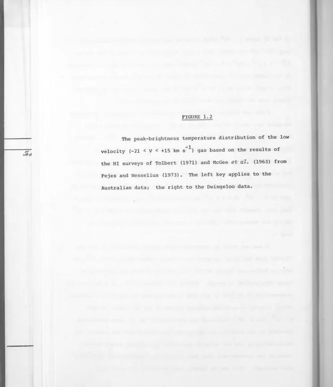
FIGURE 1.2

The peak-brightness temperature distribution of the low

-1

velocity (-21 < V < +15 km s ) gas based on the results of the HI surveys of Tolbert (1971) and McGee

et al.

(1963) from

Fejes and Wesselius (1973). The left key applies to the

[image:15.694.9.678.17.793.2]

FIGURE 1.3

Map of HI column density for the low

(lvl

~

20 km s-1)

velocity gas outside

JbJ

~

10°,

o

< -30° from Heiles and

reproduction of the hydrogen column density map of Heiles and Jenkins

(1976) for the velocity range -20 to +20 km s-l

7

On comparison of these new maps with the 820 MHz survey of

Berkhuijsen (1971), Heiles and Jenkins show that in the region of the

North Polar Spur the low velocity HI and the radio structures "are both

elongated and aligned in roughly parallel directions, with the HI lying

at higher longitudes than the radio-continuum", the association being

particularly good in the region£ ~ 30°, 10

~

b

~

60. At higher

latitudes the angular separation between the HI and continuum emission

increases to about 15° but the association nonetheless continues through

the polar regions and both the HI and continuum ridges curve back down to

b

=

50° with the HI lying some 30° towards earlier longitudes. They question the suggestion made by Wesselius and Fejes that the southern

hemisphere filament a t £ = 286°, b

=

-26° may also be associated with Loop I because of the apparent lack of associated continuum emission in

this region. They find no evidence to support the suggestion of

Berkhuijsen

et

al

.

(1971) that intermediate velocity gas is associated

with Loop I; the shape of the intermediate velocity filaments bear little

-1 0

relation to the non-thermal loop and the 40 km s component near £= 30

decreases smoothly with latitude, disappearing by b

=

40° suggesting this

material is associated with a distant spiral arm.

Heiles and Jenkins find no evidence of any correlation of HI with

-1

Loop II but show a convincing correlation of high (V ~ 70 km s ) and int rmediate negative velocity gas with the outer edge of Loop III; in both cases the HI features curve around with the edge of the non-thermal

loop.

On comparison of the HI results with optical polarization data

(Mathewson and Ford 1970; Heiles and Jenkins 1970) , show very clearly the

I

8

the local magnetic field and draw particular attention to the many

fila-ments in the region of the North Polar Spur where the polarization vectors

are very precisely aligned with the arching HI filaments. This is clearly

illustrated in Figure 1.4, taken from Heiles and Jenkins (1976) in which

the optical polarization vectors of Mathewson and Ford (1970) are

super-imposed on the hydrogen column density map for the velocity range -20 to

-1

+20 km s . From an examination of Mathewson and Ford's (1970) plots of

polarization for stars in different distance intervals they conclude that

these HI features are less than 200 pc from the Sun, a result which is

supported by interstellar Lyman-a absorption measurements in that

direc-tion (Savage and Jenkins 1972; Jenkins and Savage 1974).

Mathewson (1968) had already shown that the radio-continuum spurs

follow the flow patterns of the optical polarization vectors and used

this association to suggest that the spurs were the "radio-tracers" of

the local magnetic field, which he suggested was helical on the basis of

extensive optical (Mathewson and Ford 1970 and others referred therein)

and radio (Westerhout

et

aZ

.

1962; Wielebinski

et aZ.

1962; Brouw

et aZ

.

1962; Berkhuijsen and Brouw 1962; Wielebinski and Shakeshaft 1964;

Berkhuijsen

et

aZ.

1964; Mathewson and Milne 1965; Bingham 1966)

polarization data. He pointed out that the direction of the magnetic

field derived from optical polarization data was in agreement with that

derived from the radio polarization data in support of the Davis-Greenstein

(1951) mechanism for the alignment of interstellar grains. The optical

polarization vectors were aligned with the North Polar Spur indicating a

magnetic field tangential to it's whole length and Bingham (1967)

suggested that this was confirmed by the radio polarization data although

from his results it is not clear that the field is parallel for b

~

50°. Spoelstra (1971) has mapped the polarization in the North Polar Spur at

FIGURE 1.4

Complete sky distribution of starlight polarization

(Mathewson and Ford 1970) superimposed on the map of HI column

density for the low

<Iv!

~

20 km s-1) velocity gas, from

[image:21.700.10.674.17.806.2]

10

for b} 50° and perpendicular for b

~

50°. This field reversal he claims

(Spoelstra 1972) can be explained by an expanding shell model for Loop I

but the disparity between the field directions for b ~

so

0 inferred from

optical and radio polarization remains unexplained by any current model.

Bingham (1967) using measurements by Behr (1959) , and Mathewson (1968)

noted that in the region of the North Polar Spur, the optical

polariza-tion increases rapidly for stars at distances >100 pc and suggested that

the spur was located at a distance of 100 ± 20 pc.

Mathewson's (1968) helical interpretation of the local magnetic

field was at variance with the observed distribution of the Fraday

rota-tion measures of extragalactic radio sources (Berge and Seielstad 1967;

Gardner and Davies 1966; Gardner

et al

.

1967) , which suggested that the

magnetic field was longitudinal, directed approximately towards£= 90°

but pointed in opposite directions on opposite sides of the galactic

plane. To explain both the polarization and Faraday rotation results

Mathewson and Nicholls (1968) suggested that the helical field was

domin-ant only within about 300 pcs of the Sun, and that outside this region,

0

the field was longitudinal and directed towards £= 90 . This combination overcame the problem of the field reversal above and below the plane

-which is a natural consequence of the helical model. Gardner

et al

.

(1969) , on the basis of a more complete survey of Faraday rotation for

extragalactic sources concluded that the field was longitudinal and

directed towards£= 80° both above and below the plane with the

excep-ion of th region between £= 300° and£= 60°, where there was an

obvious deformation in the field which they suggested was probably related

to the North Polar Spur. Manchester (1972), from Faraday rotation

results for 21 pulsars concluded that the field was longitudinal and

directed towards £= 90° and in a subsequent paper (Manchester 1974) based

11

d n -- 940.

field direction towar s ~ However, in his model , results from the

region of Loop I , where the observ d rotation measur s were opposite in

sign from those expected, were excluded, and i t is essentially in this

region alone that the he~ical and longitudinal models differ.

Both the polarization and Faraday rotation results suggest there

is a local deformity in the galactic magnetic field which may be related

to Loop I, or more specifically to the low velocity gas thought to be

associated with the North Polar Spur section of Loop I.

Weaver (1977) has addressed the problem of these low velocity

filaments and their possible relation to Loop I and he shows quite

convincingly that both the low velocity gas and the local magnetic field

in this region can be understood in terms of a huge interstellar bubble

6 -1

containing some 10 M of hydrogen which is expanding at 3 km s . He

0

suggests that this bubble was produced by mass-loss from the collective

stars of the Scorpio-Centaurus association of early type stars (centred

at £ = 330°, b = 15° at a distance of· 170 pc) in agreement with the

prediction of Castor

et

aZ

.

(1975) that energetic stellar winds from early

type stars can blow bubbles in the interstellar medium. In this inter

-pretation, the (longitudinal) magnetic field, initially trapped in the

gas because of the imbalance of magnetic and hydrostatic pressure, was

drawn out along the spherical surface of the expanding shell giving rise

to the unusual distribution of the optical polarization results in this

region. The radius of this bubble is somewhat ill-defined because of the

very inhomog nous distribution of gas within the shell which Weaver

suggests is about 50 pc thick. He has assigned an average outer radius

of the order of 160 pc to the bubble, but in order to reproduce the

0ptical polarization patterns in the region 30°

~

£

~

90°, -60°

~

b

~

10°

(Mathewson and Ford 1970) , he suggests that at least part of the shell

12

this bubble from CaII interstellar absorption line data is presented in

Chapter 3. The outline of the bubble with a radius of 160 pc is

schematically shown in Figure 1.1.

Weaver (1977) has also investigated the possible relationship

between this low velocity HI shell and Loop I. He has shown that although

there is a reasonable positional correlation in the distribution of the low velocity HI features and the non-thermal emission in the North Polar

Spur section of Loop I, this correlation does not extend further around

the non-thermal loop; the centres and angular radii of the HI and

non-thermal shells differ by 6 and 15 degrees respectively and therefore they

do not project on one another. This is illustrated in Figure 1.5 in which

the other edge of the non-thermal loop is superimposed on the integrated -1 hydrogen colwnn density map for the velocity range -20 to +20 km s

(Weaver 1977). Weaver concludes that the two are not causally related and suggests that the non-thermal loop may have been dependently produced by a supernova event in the Scorpio-Centaurus association.

This correlation of an excess of neutral hydrogen with a stellar association is not unique to the Scorpio-Centaurus association. Dieter (1960) has investigated the correlation of HI with stellar associations.

She found that in 31 of the 40 associations studied, there is an excess

of HI with velocities similar to those of the associations. Heiles and Jenkins (1976) also noted the general tendency for the HI column density to be large in regions containing young stars and stellar associations, in particular the I Ori association a t £ = 205°, b = -15°, II Per at £ = 160°, b = -15° and the Sco-Cen association a t £ = 330°, b = 15°. As these associations all belong to Gould's Belt (Clube 1967), they suggest that the HI concentrations are also located within Gould's Belt.

0 0

FIGURE 1.5

Superposition of the outer edge of Loop I (black line)

on a map of the integrated HI column density for the low velocity

14

substantially older than those above, is not associated with an excess

of HI.

Heiles (1976) suggested the existence of an expanding shell of HI

in the approximate direction of the Orion and Perseus associations. This

shell, which is approximately 19° in angular radius, is centered in the

direction

i

=

198°, b

=

-40°. Heiles determined the distance to the shell

from (1) comparison of La and 21-cm column densities which placed the

shel l closer than 540 pcs, and (2) Carr interstellar absorption line data which implied that the positive velocity gas was closer than 220 pc and

the negative velocity gas was closer than 340 pc. No optical counter -parts of either the positive or negative velocity HI gas were found in

the spectra of stars closer than 130 pc and no counterparts of the

nega-tive velocity gas were found in the spectra of stars closer than 340 pc

which suggested to Heiles that (1) the shell was more distant than 130 pc

and (2) that interstellar lines are not necessarily reliable indicators

of shell material. These observations are however consistent with a

contracting rather than expanding shell as are the HI velocity patterns,

which alone do not enable a distinction to be made between expansion and

contraction.

In either event, if the interstellar lines give true estimates of distance, i t is unlikely that the shell is associated with either the

Orion or Perseus association which are located 300-500 pc from the Sun.

Heiles adopts a distance of 150 pc to the centre of the shell

(ther by placing it in Gould's B lt) and considers both a mass-loss and

supernova interpretation. The mass-loss rate required to produce the

-5

shell is 3.2d x 10 M /yr, where d i s the distance to the centre of

150 0

the shell in units of 150 pcs. This is a prohibitively high mass loss

rate for a single star unless i t is a supergiant (Hutchings 1976). Heiles

r

_ 1

15

located in the direction of the centre of the shell at a distance of 340

pc. If this star is responsible for the HI shell, i t should have a mass

-5

loss rate of 7.2 x 10 M /yr. This severe energy requirement led Heiles

0

to favour a supernova interpretation where the required energy

51 2 E

0

=

3.6 x 10 d150 ergs was more acceptable. Both interpretations are

supported by the presence of (1) Ha emission (Sivan 1974; Reynolds

et

al.

1974) , (2) diffuse soft X-ray emission (Williamson

et al

.

1974;

Naraman

et

al

.

1976) and (3) 0 VI absorption (Jenkins and Meloy 1974) in

the direction of the shell. The position of this shell is also

schem-atically shown in Figure 1.1.

Sancisi (1974) has detected expanding HI shells connected with the

associations Per 082 and Seo 082, which have radii of 20 pc and 13 pc

and expansion velocities of 5 and 3 km s-l respectively. The positions

of these shells are schematically shown in Figure 1.1. Unlike Weaver's

(1977) interpretation of the large HI shell associated with the Sco-Cen

association where the shell is produc~d as a result of mass loss from the

collective stars of the asso-iation, Sancisi (1974) suggests the reverse

generic relationship between the stars and gas: in his interpretation

the stars in the Per 082 and Seo OB2 associations were formed from

con-densations in the dense expanding shells which he suggests were produced

by supernova remnants. In both these associations the stars are located

on the outside of the expanding HI shells and although both stars and

gas expand from a common origin, the stellar component has a higher

expansion velocity than the HI component. The difference between the

expansion velocities of the stars and gas for the Per 082 and Seo 082

-1

associations is 10 and 3 km s respectively. Sancisi suggests that

~his is simply due to the fact that the HI shells will be decelerated as

they expand into the interstellar medium whereas the stellar component

will be unaffected.

r

16

Another possible coincidence between an expanding HI shell and a

stellar association was reported by Katgert (1969) who found an expanding

HI shell in the direction of the Vulpecula I association. The estimated

centre of the shel l is at a distance 2 ~ d ~ 8 kpc in the direction

0 0

£ = 61.5 , b = -0.3 ; the Vulpecula I association is located at a distance

of 2.3 kpc (Kopylov 1958) in the direction£= 60.3°, b = 0.1°.

The association of HI with the· Gould Belt system of early type

stars was pointed out by Heeschen and Lilley (1954) and Davies (1960).

It has since been confirmed by the results of McGee and Murray (1961),

Fejes and Wesselius (1973), Lindblad (1967) , Hughes and Routledge (1972),

Lindblad

et

al

.

(1973), Heiles and Habing (1974) and Weaver (1974).

Lindblad has shown that there is a ring of gas expanding in the region of

the galactic plane in the local neighbourhood. Hughes and Routledge

(1972) provided additional evidence for such an expanding ring and

Lindblad

et al

.

(1973) suggest a model in which this ring of gas is

0

expanding from a point in the direction£= 150, at a distance of 140 pc. -1

The initial expansion velocity of this ring is 3.6 km s and the

expansion age is 6 x 107 years. All investigators have associated this

expanding ring with Gould's Belt and with the expansion of the local

group of early type stars discussed by Blaauw (1956), Bonneau (1964),

Clube (1967), Lesh (1968, 1972) and Stothers and Frogel (1974) .

In an extensive study of the kinematics of stars of type 85 and

earlier north of declination -20° and within a distance of 600 pc, Lesh

derived two possible solutions for the expansion age of Gould's Belt;

when all stars were taken into account an overall expansion age of

7

9 x 10 years was found, and from an interpretation in which the

associa-tions constitute an expanding subset, an xpansion age of 4.5 x 10 7 years

was determined. Clube (1967) suggests an expansion age of 3.7 x 107 years

17

while Stothers and Frogel (1974) determine an evolutionary age for the

system of 3.0

~

0.7 x 107 years from the spectral type of the broad main

sequence turnoff near B2.5. The suggested diameters for the system are:

1200 pc (Lesh 1968), 1000 pc (Clube 1967) and 750-1000 pc (Stothers and

Frogel 1974). Stothers and Frogel suggest on the basis of the

distribu-tion of the OBl stars that the centre of Gould's Belt is located at a

distance of 212 ± 34 pc in the direction£= 180° ± 13°, b = -16° ±

s

0•

A schematic representation of this ring and the other HI shells within

Gould's Belt projected onto the galactic plane is presented in Figure 1.6.

Also shown in this figure are the positions of the six OB associations

within 500 pcs of the sun and the open Sco-Cen cluster which is

responsible for Weaver's (1977) low velocity bubble. The latter is

drawn to scale, the others are not due to lack of information. The nwnbers in brackets beside each cluster refer to the latitude of the

approximate centre of the associations.

Weaver (1974) has reexamined the model of Lindblad

et al.

(1973)

using the results of an intermediate latitude HI survey made by Weaver and Williams at Hat Creek and finds a good overall agreement with

Lindblad's hypothesis. However, at higher latitudes (-30°

~

b

~

-20°) in the longitude range 90°

~

£

~

200°, Weaver finds large amounts of negative

velocity gas which can not be explained by Lindblad's model in which the

velocities of the gas are all positive due to the fact that the Sun is

located just inside the edge of the expanding ring (see Fig. 1.6). To

explain these negative velocities, he suggests a model in which the

masses of gas which are known to exist at high z distances above the

plane (see for example Kepner 1970) become unstable and fall back to the

plane. Streams of decending gas from above and below the plane collide

and form the expanding HI ring which is observed in Gould's Belt. This

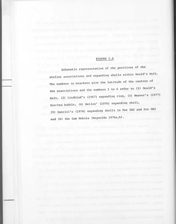
FIGURE 1.6

Schematic representation of the positions

of

the

stellar associations and expanding shells within Gould's Belt.

The numbers in brackets give the latitude

of

the centres

of

the associations and the numbers 1 to 6 refer to

(1) Gould's

Belt,

(2)

Lindblad's

(1967)

expanding ring,

(3)

Weaver's

(1977)

Sco-Cen bubble,

(4)

Heiles'

(1976)

expanding shell,

(5)

Sancisi's (1974) expanding shells in

Per OB2 and

Seo

OB2

[image:32.667.11.622.17.794.2]

-270

100

pc

1

Monoceros 081

(0)

o

1,-

~ ~

74~

\-../.

I

I

l1ao

-P,

(-17)

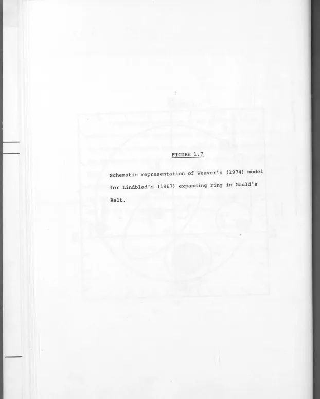
FIGURE 1.7

Schematic

representation

of Weaver's (1974) model

for Lindblad's (1967) expanding ring in Gould's

[image:34.684.12.634.16.791.2]

____________

-....

.

c:>

~~

0

20

supported by the presence of negative velocity gas in the region of both galactic poles (McGee and Murray 1961; Dieter 1964; Weaver 1974). In Weaver's interpretation, the collision of the downflowing gas streams promotes cloud formation and subsequent gravitational collapse to form stars. These new born stars reflect the motion of the gas from which they evolved thereby explaining the common expansion of stars and gas observed in Gould's Belt.

The Gum Nebula may also be another interstellar bubble produced by mass loss within Gould's Belt. Since the discovery of the Nebula

(Gum 1955) there has been considerable controversy about its origin and source of ionization.

Gum (1956) and Beuermann (1973) have suggested that it is an extended H II region ionized by the ultraviolet flux from

s

Pup, an 05 star with an effective temperature near 50,000 °K (Conti 1973) , and

y

2

Vel, a Wolf Rayet star with an 09 companion (Conti and Smith 1972). Brandt

et al

.

(1971) and Alexander

et

al.

(1971) have argued that the ultraviolet radiation from these stars is not sufficient to produce the ionization and suggest that the nebula may be a highly ionized "fossil Stromgren sphere" which was initially heated and ionized by a supernova

and is now in the process of cooling and recombining. Reynolds (1976a) has shown that the observed flux from ~ Pup and y2 Vel seems to be capable of producing most of the observed ionization and he has also shown that most of the emitting gas in the nebula is confined to an expanding shell centred in the approximate direction

t

=

258°, b

=

-1° at a distance of 400 ± 60 pc (Brandt

et al

.

1971; Gott and Ostriker

1971). This sh 11 has a radius of about 125 pc and an expansion velocity of ap roxima ely 20 km s-l Reynolds (1976b) suggests that either a

21

the stellar wind models of Castor, Abbott and Klein (1975), Reynolds -5 (1976b) suggests that the mass loss rate of s Pup may be as high as 10 M yr-1, if its mass is as large as 100 M (Conti and Burnichon 1975).

0 0

This mass loss rate, combined with the observed high stellar wind

-1

velocity of 2700 km s for s Pup (Morton 1976) is capable of producing -1 an expanding shell with radius 125 pc and expansion velocity 25 km s if

6 -3

sustained for 3 x 10 years in an ambient medium of density 0.25 cm

according to the model for interstellar bubble formation by Castor, McCray and Weaver (1975). Reynolds does not definitely conclude that

s Pup is responsible for the Gum nebula because (a) the mass loss rate for

-5 -1

s Pup may be less than 10 M yr (Lucy 1974) and (b) s Pup is not 0

centrally located ·in the Nebula. It has been suggested by Upton (1971) that s Pup may be a runaway member of the same group of B stars to which y2 Vel belongs and which Brandt

et al

.

(1971) suggest is an association within the Nebula. It may be that the combined mass loss from s Pup and this association produced the shell which is now ionized by the

ultraviolet flux from s Pup and y2 Vel. Both the supernova and mass loss models for the Gum nebula are supported by the presence of O VI absorption

lines in that direction (Jenkins 1975) although Reynolds (1976b) suggests that since comparable O VI intensities are observed for nearby stars in other directions (Jenkins and Meloy 1974) these results cannot be taken as strong support for either model. This shell and its associated stars

are also shown in Figure 1.6.

Optical rings have also been detected in other galaxies. Hayward (1964) finds rings with diameters ranging from 100 to 5000 pc in the

22

to 330 pc, are possible supernova remnants. It is unlikely that all of

these objects are supernova remnants because those with diameters less

than 100 pc should have sufficient flux at 408 MHz, if they conform to

the empirical flux-diameter relationship for supernova remnants in the

LMC established by Mathewson and Clarke (1973), to be detected in the

408 MHz survey of the Magellanic Clouds by Clarke

et al

.

(1976) . About

50% of these objects fall into this category and of these only two

(0528-674 and 0547-697) appear in the Molonglo Catalogue of Clarke

et al

.

(1976). It therefore seems reasonable to suggest that these shells may

not have been produced by supernova remnants but by mass loss from early

type stars. This suggestion is supported by recent observations of some

of these ring-like nebulae in the LMC by Lasker (1977) which show that

-1

the nebulae have expansion velocities of -30 km s In most of these

nebulae Lasker observed

[s

II] (AA6716, 6731) lines with strengths of

the same order as Ha. While strong [S II] lines have traditionally been

regarded as supernova indicators, Lasker points out that supersonic

stellar winds could equally well be the origin of the 20-40 km s-l shocks

required to produce the strong

[

s

II].

Weaver's (1977) interpretation of the low velocity gas in the

Seo-Cen association in terms of an interstellar bubble can not, by itself

explain radio-continuum Loop I. It will be shown in this thesis that

there is another HI shell centred in the Sco-Cen association which is

-1

expanding at 60 km s which has the same centre and angular extent as

Loop I implying a causal relationship between the two. As this HI shell

is best explained in terms of a supernova i t seems appropriate to briefly

review here the problems which have traditionally been associated with

23

The idea that the continuum loops were produced by supernovae has

never been unanimously accepted. A number of criticisms have been

levelled at this interpretation (see for example Sofue

et al

.

1974)

which include:

(1) The probability of finding four supernovae within 400 pcs of the

Sun.

(2) The lack of supernova remnants observed between the apparent

diameters of 5° and 40°.

(3) The contribution of supernovae to the galactic continuum emission.

(4) The lack of associated optical emission.

(1) Berkhuijsen

et

a

l.

(1971) have shown that is probability of

find-ing four supernovae in the solar vicinity is in reasonable agreement with

an outburst rate for the Galaxy of one event per 30 years if the age of

the remnants is of the order of 106 years.

(2) Sofue

et

al

.

construct a plot·of linear diameters of observed

supernova remnants as a function of distance from the Sun and show a

clear lack of supernova remnaJ)tS between the apparent diameters of 5° and

40°. Ilovaisky and Lequeux (1972) have shown the existence of an

observational selection effect which acts against the detection of weak,

extended remnants with linear diameters greater than 30 pc and suggest

that because of this there may well be a missing class of supernova

remnants. Berkhuijsen (1973) has shown that the loops conform to the

revised empirical flux-diameter ([-D) relationship of Ilovaisky and Lequeux (1972) and suggests that they belong to this missing class of

24

(3) Milne (1970) has shown, using the results for the 39 supernovae observed within 3 kpc of the Sun, excluding the galactic Loops, that if supernovae are distributed over the galactic plane with the same con-centration as in the Solar vicinity, their total contribution to the galactic radio emission is about 1%. Berkhuijsen (1971),on the other hand,has pointed out that if the distribution of supernovae is based on an estimate including the galactic Loops then supernovae should account

for about 60% of the non-thermal disc component at 820 MHz.

This is in direct contradiction to the results for M51 (Mathewson

et al

.

1972) , where the non-thermal emission is observed, not in the

luminous arms, but along the dark lanes. Sofue

et al

.

(1974) suggest

that the same is true of M31 (Pooley 1969) although this is by no means such a clear-cut case as M51. Pooley suggests that the emission in M31 originates primarily in the luminous arms and is caused either by

energetic electrons from supernovae or by enhanced magnetic field strength. In a recent review article on the radio morphology of spiral galaxies, Van der Kruit and Allen (1976) suggest that of the ten galaxies mapped with sufficient resolution (M31, M33, M51, M81, MlOl, NGC 4258, NGC 4321, NGC 5055, NGC 2903 and IC 342) to delineate spiral patterns, M51 is an exceptional case. Only in IC 342 is there definite evidence that the radio ridge is displaced toward the inner edges of the optical arms.

25

well depend on the ambient relativistic electron density and magnetic

field compression. In those cases where the relativistic electrons injected by supernova remnants is small compared to the ambient density,

the radio emission will be strongest in those regions where the magnetic field compression is highest - which corresponds to the dark lanes in M51.

(4) The lack of associated optical emission has long been a serious

criticism of the supernova interpretation, particularly on comparison

with the Cygnus Loop, an established supernova remnant which has a

comparable radio brightness to the "galactic Loops".

The first optical correlation with any of the Loops was found by

Meaburn (1967) who detected an arc of filamentary Ha nebulosity some 25°

in length partially surrounding Loop II (alternatively known as the

Cetus arc) . He pointed out that although this filament lies 20-25°

outside the radio ridge, i t nonetheless resembles the optical emission

associated with the Cygnus Loop in structure and position relative to the radio ridge. It is however about 13 times fainter than the Cygnus

Loop nebulosity and radial velocity measurements of this emission

(Losinskaya 1967; Al Sabti 1970; Elliot 1973) are not consistent with

an expanding shell source even though a small velocity gradient is

apparent in Elliot's results.

No filamentary nebulosity was detected in the region of the North Polar Spur (Meaburn 1967) . A patch of very weak diffuse emission was detected at

i

=

30°, b

=

30° but there is no evidence to suggest i t is related to Loop I. No value of surface brightness is given for this

emission but Davies

et ai

.

(1963) give upper limits for three points on the spur, indicating that the optical emission, (if any) is weaker than

that observed in the Cygnus Loop by factors of 80-340. Cruddace

et al.

lower shock velocities associated with older remnants. The optical

emission problem in Loop I will be further discussed in Section 5.5.

No correlation of optical emission with Loop III has yet been

reported.

2

The detection of soft X-rays associated with the North Polar Spur

(Bunner

et aZ

.

1972; de Korte

et aZ

.

1974; Cruddace

et

a

Z

.

1976) lends considerable support to a supernova interpretation.

Bunner

et

aZ

.

have shown the existence of an X-ray spur coincident with

the North Polar Spur along i t's whole length. Cruddace

et al

.

have shown

that the X-ray results are consistent with a supernova remnant having

just entered the radiative cooling phase. They estimate the initial

5 energy of the event, which occurred,they suggest, between 1.4 x 10 and

5 51 53

3.8 x 10 years ago, was between 1.5 x 10 and 4. x 10 ergs. They

also note the presence of a weak X-ray source 3Ul439-39 close to the

0

centre of Loop I - the error boxes are 3.8 apart.

Although considerable theoretical and observational support has

now accumulated for the supernova origin of the galactic loops, the lack

of associated HI in the case of Loops I and II and associated optical

emission in the case of Loops I and III remains a serious difficulty.

Loop I cannot be fully investigated in HI until southern hemisphere

observations comparable to those of Heiles and Habing (1974) are available.

It is the purpose of this thesis to provide these observations and to

examine this problem further . It will be shown that there is an

associ ion of intermediat velocity HI with Loop I which can best b

explained by a supernova event which is consistent with the results from

synchrotron emission, X-ray emission, radio and optical polarization,

optical emission and the low velocity interstellar HI bubble (Weaver 1977)

27

CHAPTER 2

A

S O U T H

E

R

N

S K Y H I

S

U R V E Y

2

.1

IntI'oduction

An extensive, fully sampled neutral hydrogen (HI) survey of the

sky outside lbl ~ 10°, dee~ -30° within the velocity range -92 to +75

-1

km s was made by Heiles and Habing (1974) using the 85-ft telescope at

Hat Creek. Heiles and Jenkins (1976) presented the results of this

survey in the form of photographs of hydrogen column density for selected

velocity intervals which showed very clearly the complex distribution of

low and intermediate velocity gas in the northern hemisphere. Perhaps

the most striking result of this survey was the detection of many HI

features of large angular extent.

It is naturally of interest to establish whether or not this

type of structure is reflected in the southern hemisphere, but the

limited data available prior to 1974 for the southern sky was not

sufficiently comparable to the combination of sensitivity, velocity

coverage and velocity and spatial resolution used in the Heiles and

Habing (1974) survey to make a detailed comparison. The only fully

sampled HI survey of the southern sky, made by McGee and Murray (1961)

was sensitivity limited by a super-heterodyne receiver which had a

system noise temperature of 800°K. The high sensitivity Magellanic Stream

survey (Mathewson

et

al

.

1974) covered the southern sky south of

declination -37.5°, but had a coarse grid spacing (2.5°) and was recorded

on photographic film. Furthermore, because of the method of recording,

much of the information on the low velocity material was lost. A fully

sampled survey of the southern sky is underway at the Argentinian

high velocity resolution for the limited velocity range of

-1

-40 ~ V ~ 40 km s .

This thesis presents the results of a southern sky HI survey

south of declination -30°, excluding the strip bounded by lbl < 10°

28

(this strip has been surveyed by Kerr and Bowers 1977), which attempt s to

combine high sensitivity, large velocity coverage and reasonably high

spatial resolution. The results of this survey have been combined with

those of Heiles and Habing (1974) to produce total sky maps of the

neutral hydrogen distribution outside lbl < 10° for the velocity range

-90 to +70 km s-1.

2.2 Equi

pment

The survey was made using the 60-ft telescope at Parkes Radio

Observatory, CSIRO, which has a HPBW of 48 min arc at 21-cm. The H-line

receiver had a parametric front end which gave an average system noise

temperature of 100°K. The receiver back end was the Parkes 64-channel

spectrometer (Batchelor

et

al

.

1969) and the channel width and spacing

h b k 7 km S-1

were c osen to e 33 Hz or Profiles were obtained by

frequency switching between a signal and reference spectrum with the

reference spectrum located on the negative velocity side of the signal

spectrum to prevent signal contamination from the Magellanic Stream

(Mathewson

et

al

.

1974). The system was calibrated approximately once

every two hours using a noise diode at the vertex of the paraboloid

which was calibrated at four day intervals against Virgo A and was found

to remain constant to within 8% over the duration of the survey. From

an analysis of the records, the minimum detectable signal was found to

0

FIGURE 2.1

30

20

OK

Tb

10

1=297.L.

b=-27.0

-210

-140

-70

0

70

140

VELOCITY

(km

s

1}

30

2

.

3

Ob

s

e

rvati

o

ns

Drift scans at constant declination were used with continuous

integration in right ascension for

-so

0

~

6

~

-30°. For

6

<

-so

0 , a

grid of positions spaced one degree apart in declination and one

beam-width apart in right ascension were observed. The integration time per

profile in both cases was 270 seconds.

The survey was made in two parts:

(1)

( 2)

b ) -25°,

b < -25°

6

~ -30 0

0

In part (1) the scans were spaced at 1 intervals in declination

-1

and the velocity coverage was from -148 to +300 km s . In part (2) the

0 -1

scan spacing was 2 and the velocity coverage was from -230 to +218 km s .

The parameters of the survey are sununarized in Table 2.1; those of Heiles

and Habing (1974) are included for comparison. Profiles from the regions

of overl p between the two surveys were used to standardize the southern

survey against the northern survey which in turn was standardized against

the standard region SB (Harten

et al

.

1975) .

2

.

4

Data Reduction

The original profiles contained an instrumental second order

base-line which was removed by the following procedure.

The profiles were obtained using drift scans at constant declina

-tion ov r periods in right ascention which were typically about six hours

in length; each such group of profiles constitutes a file, of which there

numbered 181 with an average of about 80 profiles per file. These

profiles ar , of course , in time order and i t was assumed that the

instrum ntal baseline B. (f) for profile number i could be expressed as

TABLE 2.1

SUMMARY OF OBSERVATIONAL PARAMETERS FOR THE SOUTHERN SKY HI SURVEY AND THE HI SURVEY OF HEILES AND HABING (1974)

HPBW Integration Grid Velocity Velocity Region

Survey (min time spacing coverage resolution surveyed

arc) (secs) ( 0) (km s- 1) (km s-1) co)

Intermediate

48 270

M

=

1 -148:,: V:,: 300

0

:,: -30

latitude

7.0

lbl

~ 10

b

~ -25

High

48 270

M

=

2 -230 :;:: V:,: 218 7.0

0

:;:: - 30

latitude

b

< -25

t,Q,

=

0.3 - 42 :,: V :,: 43 1. 2 Heiles and

36 80 cos

b

- 92:;:: V < -42

0

> -30

Habing

_D.b

₌

_{0.6 43 < V :,: 75} 6.4

l

b

l

~ 10

w

32

B. (f)

=

z.

+ S(t)(f-f ) + C(t) (f-f ) 2

l l 0 0 (1)

where S(t)

=

s

+ Sit+ S2t2

0

(2)

and C (t) C +Cit+ C2t2

0

That is, the slope S(t) and the curvature C(t) were assumed to be smooth functions of time but the zero level Z. was assumed to fluctuate randomly

l

from one profile to the next; these assumptions were based on visual inspection of the original profiles and in the kind of receiver instabilities to be encountered. Z, Sand C were computed for each profile, as described below, and the parameters in equation (2) were fit using the least squares technique. Sand C were plotted and visually examined for each file; for many files these quantities suffered one or more discontinuities within the file, and the least squares technique was performed in a piece-wise fashion. The second order terms 52 and C2 were included only for a small minority of files, based on visual inspection

of the plots of Sand C.

Sand C were computed for each profile in the following way. For each file a "safe" velocity range was selected in which there should be little HI, based on the knowledge obtained by the previous coarse grid

7 0 .

HI surveys in the southern sky (Mathewson

et

a&

.

1974 and a 2.5 grid

survey made by the author of the region -75°

~

O

~

-30°, 06 00 ~RA~ 20 00) . Sand C were obtained by a least squares fit to the channels within the safe velocity range. For some files, the plots of Sand C displayed systematic trends which might have resulted from the 21-cm line; these profiles were not included in the fit for equation (2) unless visual inspection of the profiles proved that the trends were of instrumental origin. For all least-square fits, data points having residuals larger

33

The zero level for each profile Z. was derived by first applying

1

the corrections S(t) and C(t) and then averaging the first four good channels at the end(s) of the profiles. For profiles in files for which the safe velocity range included channels on both extreme ends of the profile, channels on both ends were included. However, for some files, the safe velocity range included only the channels on the negative velocity side of the profile, and for these only channels on that end were included so that their baseline errors are larger.

For most profiles baseline curvature and slope amounting to

. 0 0

typically about 1 K were reduced to less than 0.2 K; in some cases, mainly where the receiver was particularly unstable or near the most

intense parts of the Magellanic Clouds, the baseline is less accurate.

2

.

5 Data Presentation

The data were used to generate complete sky photographs of the neutral hydrogen column density outside lbl < 10° for selected velocity intervals compatible with the data of Heiles and Habing (1974). The photographs were produced on the PDS microphotometer at U.C. Berkeley using the technique outlined by Heiles and Jenkins (1976). Each map is shown in two projections; a longitudinal projection and stereographic projections centred on the Galactic poles. In the stereographic

projection, the outer edge of the picture is lbl

=

10° and longitude is measured anticlockwise around the edge. Each of these stereographic projections is enclosed by a frame of dots. All four sides are identical with each side consisting of a series of seventeen dots. The central, or ninth dot on any side corresponds to lbl

=

10° and the first or last dot on the same line corresponds to lbl

=

90°. The interval between

34

The total sky distribution of the HI column density for the low, and positive and negative intermediate velocity gas is shown in longitud-inal projections in Figures 2.2 and 2.3a,b respectively. The velocity

-1

range for the low velocity gas is -20 ~ V ~ +30 km s This rather high -1

upper limit of +30 km s was selected for the low velocity gas because -1

the +20 km s limit used by Heiles and Jenkins (1976) was not adequate

for all areas in the southern hemisphere, in a few cases, for example at

0 0 -1

t

=

240, b

=

-21 , velocities at peak temperature of up to +20 km s are observed for the low velocity gas. The velocity limits for the positive and negative intermediate velocity gas are +30

~

V

~

+70 km s-l

-1

and -90 ~ V ~ -20 km s respectively.

These same total sky maps are presented in stereographic project-ions in Figures 2.4a-d and 2.5a-d for the northern and southern galactic

hemispheres respectively. Working clockwise from the top left hand corner of these pictures are (a) the low velocity gas; (b) negative

intermediate velocity gas; (c) positive intermediate velocity gas and (d) positive and negative intermediate velocity gas. A coordinate system for these stereographic projections is presented in Figure 2.6.

The above pictures give little information regarding the hydrogen column density at a given position. A contour map of the hydrogen column

-1

density for the complete velocity range (-92 ~ V ~ +75 km s ) of the Heiles and Habing (1974) survey was presented by Heiles (1975). Contour maps for selected velocity ranges in the southern hemisphere are presented

in Figures 2.7 to 2.10. The longitudinal projections (Figs. 2.7a to

20 -2 o

2.10a) show the column density in units of 10 atoms cm down to b

=

-75 and the polar projections (Figs. 2.7b to 2.10b) cover the latitude range -90°

~

b

~

-75° for the corresponding velocity intervals. These are: -20 ~ V ~ +20 km s -1 (Fig. 2.7), -40 ~ V ~ +40 km s -1 (Fig. 2.8),

-1 -1

FIGURE 2.2

Longitudinal projection for the total sky distribution of

the HI column density in the velocity range -20 { V {

+

30 km s-l

from the combined results of the Hat Creek Survey (Heiles and Habing

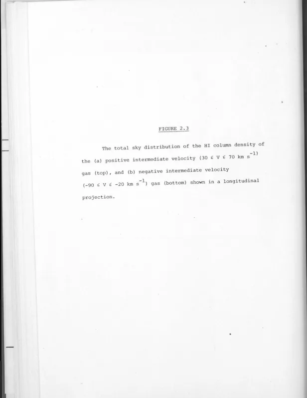
FIGURE 2. 3

The total sky distribution of the HI column density of

the (a) positive intermediate velocity (30

~

V

~

70 km s-l)

gas (top) , and (b) negative intermediate velocity

(-90

~

V

~

-20 km s- 1 ) gas (bottom) shown in a longitudinal

[image:54.668.1.617.16.815.2]

FIGURE 2.4

Stereographic projections of the N

8 distribution of low and intermediate velocity gas in the north galactic hemisphere.

Working clockwise from the top left hand corner are: (a) the low

velocity gas (-20

-1

~ V !; 30 km s ) ; (b) negative intermediate

velocity gas (-90

~

V !; -20 km s-1); (c) positive intermediate

velocity gas (30

~

V !; 70 km s-1) and (d) positive and negative

[image:56.688.0.671.13.806.2]

FIGURE 2.5

Stereographic projections of the NH distribution of the

low and intermediate velocity gas in the south galactic

hemisphere. working clockwise from the top left hand corner are: -1

(a) the low velocity gas (-20 f V f +30 km s ) ; (b) negative -1

intermediate velocity gas (-90 f V f -20 km s ) ; (c) positive intermediate velocity gas (30

~

V

~

70 km

s-1

) and (d) positive

[image:58.678.1.618.18.801.2]

[image:60.699.11.681.16.783.2]

FIGURE 2. 6

.

270

0

1-t-+-+-+-+-t-~~-+-+-+-+-+--+--1 180

-t

FIGURE 2.7a

Contour map of the integrated HI column density for

-1

the velocity range -20

~

V

~

+20

km

s

, for

20

0 o 2 , 6 a 10 11 a ,a

l•10"o1orn1 crn 11

-20

-40

-60

FIGURE 2.7b

Contour map of the integrated HI column density for

the velocity range -20 { V {

-1 0

+20 km s , for b { -75

0

0

"'

0

"

...

..,

I

I

\

0

0

"'

~-1

,D

"'

E

~2

0

0

N~

)(

o-0

"'

..,

I

\

\

-~

0

\

\

0

0

0

"

N

•o

FIGURE 2.Ba

Contour map of the integrated HI column density for

-1 0

the velocity range -40 ~ V ~ +40 km s , for b ~ -75

of the Southern Sky Survey.

FIGURE 2.Bb

Contour map of the integrated HI column density for

-1 0

o"'

"

I

-00

FIGURE 2.9a

Contour map of the integrated HI column density for

-1 0

[image:70.691.4.663.20.805.2]

4

0

20

0

-

20

-

40

•

- 60