Risk sharing and EMU

S

TRATHCLYDE

D

P

E

RISK

SHARING

EMU

B

JACQUES

MÉLITZ

UNIVERSITY OF STRATHCLYDE

,

-

&

N

.

04-02

D

E

U

S

RISK SHARING AND EMU

Jacques Mélitz

University of Strathclyde, CREST-INSEE, and CEPR

Late February 2004

Abstract: What are the prospects that risk-sharing in the EMU will ever attain the

levels in the U.S.? So far as the risk-sharing in the U.S. depends on in-terregional transfers through the budget of the federal government, those prospects are poor. So far as the risk-sharing in the U.S. takes place though market channels, they are much better. The paper ad-dresses the theory and evidence on the subject. Asdrubali, Sørensen and Yosha provide a general framework of analysis. One issue is the adequacy of the framework. With respect to the evidence, the EMU still lags far behind the U.S. as regards the pooling of risks through portfolio diversification. But there already seems to be little to distin-guish the euro zone from the U.S. concerning the ability to borrow to smooth shocks. Thus, the extent of risk-sharing via credit – a matter that Asdrubali, Sørensen and Yosha raise – is of special interest. Fur-ther, the empirical evidence indicates that the progress of European economic and monetary integration over the last decade has increased the symmetry of business cycles. However, this could be a sign of re-maining capital-market imperfections, though that is only one interpre-tation.

JEL Classification: F02, F15

Keywords: Risk sharing, EMU, fiscal federalism, portfolio diversification, current account balance.

In rich countries, the separate regions share risks with one another to an important degree. On

the other hand, the member countries of the EMU do not pool risks nearly as much as regions

within countries do. The main point of comparison is always the United States. When a

re-gion of the U. S. suffers an adverse shock, its tax contributions to the federal budget diminish

and it receives federal help in other ways. Federal transfers and grants stay up, and some of

them may even rise. The region thereby obtains relief. In the case of an EMU member in

dif-ficulty, no similar assistance will come from the EU budget. In this respect, the member

coun-tries of the EMU are at a distinct disadvantage relative to the regions of the U.S. Short of an

unforeseen reform in the EMU, this will continue.

However, Americans also share risks in other ways that Europeans can hope to emulate in the

future. There is a significant cross-ownership of claims to property in the U.S. When an

ad-verse shock hits a U.S. region, the residents will share the damage with the non-residents to

some extent because many holders of the income claims to the output live in different regions.

By promoting capital market integration, EMU may encourage risk-sharing of this sort. In

addition, the residents in a region in the throes of a recession will find it easier to borrow from

their compatriots in other sections because of a single money. EMU should clearly encourage

risk-sharing of that sort too. Many theorists would not refer to risk-sharing in this last

in-stance. They would reserve the term for insurance coming from portfolio diversification

(while occasionally allowing the term to cover also aforementioned transfers through the

cen-tral-government budget). However, under autarchy, residents would not be able to smooth

shocks via credit. Therefore, there is little harm in broadening the concept of “risk-sharing” to

encompass credit transactions as well.

An important contribution by Asdrubali, Sørensen and Yosha (1996) (hereafter ASY)

pro-poses a framework that is capable of analyzing all three previous mechanisms of risk-sharing

in an integrated way: namely, (1) transfers through the upper-government budget; (2)

insur-ance or cross-ownership of income claims to output; (3) credit or borrowing and lending. The

authors estimate the risk-sharing via these three mechanisms to be, respectively, 13, 39, and

23 percent in the U.S. The last two of these numbers – those regarding the risk sharing

through market channels – add up to 62 percent, implying considerable smoothing of output

shocks. If these estimates can be taken seriously, the prospects for risk-sharing in the EMU

are much better than they otherwise appear. Thus, the logic and the accuracy of ASY’s

esti-mates are important.

In the first section, this paper will consider the extent of risk-sharing via the federal budget in

the U.S. Some basic related questions still remain open on this subject. The next section will

proceed to examine the risk-sharing in the U.S. via cross-ownership of claims to output and

via credit. The discussion will then take up the prospects for higher risk-sharing through the

two market mechanisms in the EMU. The final section will move on to examine the impact of

EMU on the total insurable risks. This next matter will bring us into familiar territory,

con-cerning the degree of asymmetry of the shocks.

The major conclusions – at least a few of them – may be mentioned at once. First, the broad

differences in the literature in the estimates of risk-sharing via the federal budget in the U.S.,

going from 40 percent to only 10, are still ill-understood. These differences really have little

to do with the use of levels or first differences in the econometric analysis, or redistribution as

opposed to stabilization. They stem from the accounting instead. However, the accounting

raises some basic and neglected conceptual issues. The smoothing of regional shocks coming

from this public source is around 12-15 percent overall. With respect to the market channels

of risk-sharing, ASY’s numbers for the U.S. are probably exaggerated. The pooling of risks in

the EMU still lags behind the U.S. and will do so for a long time to come. But there already

seems to be little to distinguish the euro zone from the U.S. in regard to the ability to borrow

to smooth shocks. Thus, the extent of risk-sharing via credit – an issue that ASY do very well

to raise – is of considerable importance. Finally, the empirical evidence indicates that the

pro-gress of European economic and monetary integration over the last decade has increased the

symmetry of business cycles. But this poses a general conceptual problem. With the advance

of capital market integration, people should be willing to accept more output risks since they

can share the risks more easily. From this perspective, the increase in the symmetry of

busi-ness cycles in the EMU could be a sign of remaining capital-markets imperfections. This is

not the only reading, but it is a possible one. The interpretation would mean that the

increas-ing symmetry of business cycles in the Euro zone signals a poor allocation of the risks

be-tween individuals.

I. Risk-sharing via the central government budget in the U.S.

General downturns in economic activity in a country tend to raise deficit spending by the

cen-tral government. Such responses by the government obviously say nothing about the

smooth-ing of regional shocks, or the smoothsmooth-ing of movements in the output of some regions relative

to others. All relevant studies of regional stabilization through the federal budget in the U.S.

necessarily try to control for this problem. They do so either by introducing a separate fixed

effect for each period (von Hagen (1992), ASY (1996)) or else by using ratios of regional

values to national averages (Sala-i-Martin and Sachs (1991), Bayoumi and Masson (1995)).

Either procedure comes to about the same. The studies also proceed mostly by regressing a

regional output variable or a regional income variable following net federal transfers on the

same regional variable, prior to net transfers. Sala-i-Martin and Sachs (1991) (hereafter

SiMS), who opened the discussion, measured both the aforementioned dependent and

inde-pendent variables in levels. These two authors also used personal income figures. They

re-ported 40 percent stabilization. An influential contribution by von Hagen (1992) then

fol-lowed quickly, and used first differences and real gross product figures. von Hagen got 10 per

cent stabilization instead. He also ascribed the enormous difference in his results to his use of

first differences rather than levels. Further, he suggested that his choice of first differences is

the appropriate one in studying stabilization, whereas SiMS’s choice of levels pertains more

closely to redistribution instead. This diagnosis has made a lasting impression. To the

con-trary, however, the use of levels or first differences is not central. Moreover, there is little

difference between redistribution (properly measured) and stabilization in the U.S.

I will now briefly display the validity of these conclusions. Let Xit be either per capita

sonal income in region i in year t divided by per capita personal income across the nation in

year t, or else per capita gross product in region i in year t divided by per capita gross product

in the nation. In either instance, the weighted sums of Xit values across the regions, based on

population weights, equal one. Let Yit be the corresponding values of Xit after the addition of

net transfers per capita by the national government. Consider next equations (1) and (2),

con-taining a disturbance term (µit or νit, as the case may be).

Yit = αi + βsXit + µit (1)

∆Yit = di + βs∆Xit + νit (2)

Equation (1) reflects SiMS’s choice in analyzing stabilization in the U.S. Equation (2) reflects

von Hagen’s. In both cases, βs relates to stabilization. If we take equation (1) in first

differ-ences, all the regional constants αi drop out. Therefore, equation (2) does not follow exactly

from equation (1), but rather supposes a possible regional drift or trend, di, in the Xit values

over time. However, in the absence of such drifts or trends in the Xit terms (if di = 0), equation

(2) is simply equation (1) in first differences (with ∆µit = νit). Further, if, in addition, the

dis-turbances µit possess certain well-known statistical properties, then the estimates of equations

(1) and (2) will yield identical estimates of βs. Suppose that a rise (fall) of $1 in Xit always

yields a rise (fall) of Yit of 90 cents. Then βs is 0.9, and stabilization is 0.1. The measure of

stabilization is therefore 1–βs.

Table 1 provides separate estimates of 1–βs for equations (1) and (2), and reports these

esti-mates separately in case of SiMS’s measure of Xit and von Hagen’s. In all the estimates, the

U.S. is broken up into 48 regions: the 50 states minus Alaska and Hawaï. The interpretation of

transfers from the central government is always the same: namely, direct taxes plus social

insurance plus transfers to persons and grants to states. As can be seen, in the event of the

gross product measure (von Hagen’s), the estimates in levels and first differences are virtually

identical. In case of the personal income one, the two estimates differ by 7 percent or less than

half of the total (whether 0.2 or 0.27). But the differences between the two measures of Xit

look important on the whole. We will come back to this last point shortly.

There is a third estimate in the table resting on a separate equation, owing to Bayoumi and

Masson (1998):

(3) Y_i=α_d +β_dX_i +η_i (3) In this next example, X_iand Y_i represent averages of Xit and Yit over the whole study period.

Consequently, unlike βs, the coefficient βd does not reflect any movement over time, but

re-lates strictly to cross-sectional differences between regions over the entire study period.

Ac-cordingly, the coefficient can be seen as pertaining to redistribution.1 _{The idea of separate}

coefficients βs and βd, for stabilization and redistribution, also makes perfect sense.

It is easy to imagine countries where taxes would be moderate yet highly progressive,

redis-tributive spending would be high, and there would be no unemployment compensation, no

temporary subsidies, no temporary tax breaks. Consequently, redistribution (βd) would be

strong and stabilization (βs) weak. Alternatively, we can imagine the opposite: countries with

strictly proportional taxation, lots of temporary aid in case of disasters but no permanent

as-sistance to the poor. Then βs would be high and βd low. It is clear from the table that the U.S.

belongs to neither of these two instances. For this country, βs and βd are much the same.

Therefore, not only is there little notable difference in levels and first differences for

stabiliza-tion in the U.S., but there is little indicastabiliza-tion of higher redistribustabiliza-tion than stabilizastabiliza-tion.

On the other hand, depending on personal income or gross product data, the stabilization and

redistribution estimates in Table 1 do differ widely. They go from 12 to 14 percent to 20 to 27

percent. The major contributors to the discussion of stabilization in the U.S. also divide right

down the middle about the right measure to use. Bayoumi and Masson (1995) and Obstfeld

and Peri (1998) follow SiMS in adopting the personal income measure, while Goodhart and

1 _{As noted by Mélitz and Zumer (2002), equations (1) and (3) can be jointly derived from the}

more general hypothesis:

Y_it=α_d+β_dX_i+β_s(X_it −X_i)+ε_it

(The sum of equations (1) and (3) gives rise to this last equation with αi equal Y X_i − β_{s i}and

ηi+µit equal εit.) As is also well known from panel data econometrics, estimates of this more

general equation or separate estimates (“within” and “between”) of equations (1) and (3) yield identical estimates of βs and βd .

Smith (1993) and ASY (1996) opt for von Hagen’s gross product one. There is also an

occa-sional difference in the measure of net transfers. Those accounting choices are the critical

ones. The combination of a narrow measure of net transfers and a wide measure of regional

activity (gross product) leads to low estimates of stabilization, while the combination of a

wide measure of net transfers and a narrow one of regional activity leads to high estimates of

stabilization. Table 2 makes the point.

The top half of the table relates to stabilization, the bottom one redistribution; the left-hand

side relates to personal income, the right-hand one to gross product. In the case of either top

or bottom half, lower rows (numbered 1, 2, 3) concern successively larger measures of net

transfers. If we look down to lower rows, we find that the estimates of βs and βd successively

rise. As regards the differences left and right, the figures for gross product are far higher than

those for personal income. If we compare the columns on the left with the corresponding ones

on the right, we find the estimates of βs and βd on the right consistently lower. SiMS

com-bined the highest measure of net transfers (rows 3) with the lower measure of Xit. von Hagen

combined a lower measure of net transfers (rows 2) with the higher measure of Xit. That is the

key to the difference in the estimate.

It might seem that the critical choice is really that of Xit, and the measure of net transfers is

subordinate as long as we limit the choice to rows 2 and 3. But that is an accident of the U.S.

example. With regard to Canada, for instance, including or excluding federal grants to the

provincial governments (choosing between rows 2 or 3) makes as much difference as

choos-ing personal income instead of gross product accountchoos-ing. In the case of gross product

ac-counting (von Hagen’s choice), the estimate of βs is only 3 to 4 percent for Canada under the

narrower measure of net transfers in rows 2, while adding the federal grants to the provincial

governments raises the estimates of βs to 13 or 14 percent (depending on levels or first

differ-ences). Likewise, when we pass from the measure of net transfers in rows 2 to the wider one

in rows 3, βd goes from 16 to 30 percent in Canada (see Mélitz and Zumer (2002)).

What then is the right choice of accounting? We can think of regional income as the

produc-tion in the region. Then the income belongs partly to the residents of other regions. Or else we

can think of regional income as the income of the residents. Then some of the income stems

from production in other regions. It is difficult to see why one choice or the other should be

the only right one. For example, consider a state like Louisiana where the population is poor

but the output per head is high relative to the rest of the U.S., or another like Florida where

much of the population is retired and living on income coming from elsewhere. To focus

exclusively on gross product is to put the emphasis on the activity in the region: the

productivity of firms, employment, infrastructure, etc. But that glosses over the issue of the

welfare of the residents. Why not consider the stabilization and redistribution in the region

from the standpoint of smoothing and equalizing these people’s revenues and their

consump-tion instead? Investigators take one view or the other, but there is much to be said for either

view, and it may therefore be best to keep both of them in mind. The next question is whether

regardless of the choice of measure of Xit, the same measure of net transfers should serve.

If the issue is the redistribution and stabilization of the disposable gross product of the

re-gions, it seems clear that all the central-government net transfers are relevant. Regardless

whether the transfers are direct or indirect, all of them support local activity. However, if the

question relates to the redistribution and stabilization of the disposable personal income of the

residents, then including the transfers to the regional governments is not necessarily correct.

True, the residents of a region derive benefits from central-government subsidies to their local

governments as well as such direct subsidies to themselves, since the ones to the regional

governments provide them with better services of transportation, recreation, communication

and so forth. But so do tourists, transients and commuters. More important, if the net

trans-fers to the regional governments are to be included in the residents' disposable income, the

question is why the entire flow of similar services that the residents get from local firms is not

incorporated there as well (but only in so far as those services correspond to payments of

wages and interest to residents). Much of the capital in a region belongs to the residents.

Therefore, the retained earnings of local firms belong disproportionately to them too. Yet

those earnings do not enter into their personal income. If there are to be any imputations for

transfers, should not those retained earnings be imputed to them too? Finally, it seems

incon-testable that if purchases from local firms by municipal and state governments are included in

the residents' disposable income when the central government subsidizes them, those

pur-chases must always be included there.

In other words, the issue is one of coherence in accounting: the concepts of income before and

after net transfers must agree. The choice of a broad measure of net transfers requires a

corre-spondingly broad measure of income. As already shown, combining a broad measure of net

transfers with a narrow measure of income will systematically swell the estimates of βs and

βd. On these grounds, the proper measures of βs and βd would seem to be those in rows 2 in

case of personal income accounting and in rows 3 in case of gross product accounting. If we

also accept the usual preference for the estimates of stabilization in first differences, that puts

the estimates for the U.S. in the range of 12 to 15 percent for βs and 14 to 18 percent for βd.2

II. Interregional risk-sharing via credit and cross-ownership of property in the U.S.

High estimates of interregional risk sharing via the federal government in the U.S. possibly

dash any hope that risk-sharing in the EMU will ever attain the U.S. level. However, similarly

high estimates of risk-sharing through market channels can even kindle such hope. Let us then

examine the basis for ASY’s estimate that the U.S. regions share over half of the insurable

2 _{Decressin (2002) raises an important separate issue. National governments make many}

pay-ments to national civil servants, and public and private firms rather than households and lower-level governments. These payments do not always show up in the official regional ac-counts – less so in centrally organized countries than federally organized ones. Furthermore, some of the spending in question may be on private goods, such as health and education, and those goods (or services) may be distributed based on a principle of equal access by everyone. Consequently, some redistribution may result from the relevant spending and possibly some stabilization too. But without a special decomposition of the relevant national spending by region, the analyst will miss the associated regional redistribution and stabilization. Decressin makes the right correction for Italy. He also thinks that the correction argues in favor of gross product accounting. The latter is difficult to see. Sicilians benefit greatly from education and health services that they receive privately from teachers and medical workers at national ex-pense. Why should this lead us to favor analyzing the stabilization and redistribution of Sicil-ian output per head rather than SicilSicil-ian personal income?

risks to output with one another via private channels.

Consider a panel of regional data consisting of per capita output Yi, per capita personal

in-come PIi, per capita disposable income DIi, and per capita consumption Ci, all stated in real

terms. The index i refers to the region. ASY start with the identity

Y Y PI

PI DI

DI C C

i i

i i i

i i

i

= (4)

Next, they take logarithms and first differences:

∆log Y_i= (∆logY_i −∆logPI_i) + (∆logPI_i −∆logDI_i )

+ (∆logDI_i −∆logC_i) + (∆logC_i ) (5)

Then they multiply both sides of equation (5) by ∆log Y_i, and subsequently subtract the means of all five terms over the study period, the one on the left and the four in parentheses

on the right. Following, they take expected values. The result is the variance of the change in

the log of Yi on the left and the sum of the covariances of this term with, respectively,

∆logYi−∆logPIi, ∆logPIi −∆logDIi, ∆logDIi − ∆logCi, and ∆logCi, on the right. Finally, they

divide both sides of the last equation by the variance of ∆logYi. This yields:

1=β_K+ β_G +β_C+β_U (6)

The covariance/variance β terms in equation (6) correspond exactly to OLS estimates

of the following regressions:

∆logY_i −∆logPI_i =α_K+β_K∆logY_i +µ_iK

∆logPI_i −∆logDI_i =α_G+β_G∆logY_i +µ_iG (7)

∆logDI_i −∆logC_i =α_C+β_C∆logY_i +µ_iC ∆logC_i =α_U+β_U∆logY_i +µ_iU

Consequently, ASY estimate all four equations. Before doing so, they introduce a fixed effect

for each year in order to take account of the general growth rate in per capita output over all

of the regions at each date. Then as a final and separate step, they assign a specific empirical

interpretation to βK, βG, βC and βU. They interpret βK as a measure of the smoothing of

re-gional shocks to per capita rere-gional output through the cross-rere-gional ownership of claims to

output; βG as a measure of the smoothing of these shocks through the central government

budget; βC as a measure of the similar smoothing coming from interregional credit; and βU as

a measure of the unsmoothed portion of the regional shocks. The value of the whole exercise

evidently depends on these last interpretations.

Upon consideration, it is clearly possible to question the interpretations. Take the equation

for PIi/Ci, concerning household saving. Suppose there are changes in the age structure of

households between regions. This is only reasonable since ASY’s study covers 37 years

(1963 to 1990). Those demographic changes may well induce changes in PIi/Ci independently

of any movements in Yi. Subsequently (and as a separate point), those changes can also have

some reverse effects on Yi. So far as this happens, the estimate of βC will evidently not

con-cern smoothing of output shocks at all. As regards Yi/PIi, suppose that firms sometimes make

investment decisions based on anticipated changes in relative demand for their produce. Once

again, Yi/PIi may change independently of changes in Yi and, additionally, there may be

re-verse effects on Yi. Then a similar problem as before arises: the estimate of βK will not reflect

any smoothing by firms. Yet ASY do provide notable support for their interpretation.

First, as regards βG, their procedure evidently nearly reproduces the one described before for

estimating risk-sharing through the federal government budget based on gross product

ac-counting (and the use of first differences). Quite apart from this mere issue of precedent, the

difference between personal income and disposable income is indeed likely to reflect

essen-tially the rules governing taxes and transfers.3 _{The problem of interpretation is far more}

se-vere with respect to βC and βK. As regards these two coefficients, underlying ASY’s

interpre-tation is the idea that all risks associated with asymmetric shocks to output should be possible

to pool since they are perfectly negatively correlated with one another. However, as ASY

explicitly point out, so far as such risks are not pooled and remain uninsured, it should be

3 _{Nonetheless, there does remain a possibility of reverse causation or simultaneity bias in}

es-timating βG based on equations (7) the way ASY do, just as there was before (unmentioned)

in estimating βs based on equations (1) or (2) like earlier authors. As a result, both SiMS and

Bayoumi-Masson used instrumental variables to correct for the problem. But Mélitz and Zumer (2002) found that the correction makes hardly any difference.

ier to obtain credit for smoothing those of the associated shocks to output that are temporary.

Hence, less persistent shocks should lead to higher estimates of smoothing via credit. Based

on this logic, ASY use the Campbell-Mankiw (1987) index to distinguish the persistence of

shocks affecting different states. They also employ averages over successively longer periods

to do the same. In addition, they classify the U.S. states according to the degree of the

sensi-tivity of their industrial structure to cyclical movement and therefore their proneness to short

swings. These tests generally confirm ASY’s hypothesis that more persistent shocks increase

βK relative to βC. This would then seem to indicate that higher values of the ratio βK/βC

sig-nify greater reliance on insurance relative to credit in smoothing regional output shocks. On

this ground, ASY’s estimates of risk-sharing through market channels in the U.S. deserve

serious attention.

Nonetheless, there are two reasons why those estimates are too high. First, ASY understate

βU. Second, they neglect the fact that βK and βC partly reflect autonomous smoothing within

the regions themselves having nothing to do with risk-sharing.

On the first point, the importance of βU in assessing βK + βC should be clear. Based on the

identity (6), βK + βG + βC + βU equals one, and therefore every percentage point of βU means

a percent less risk sharing. In order to estimate βU, as mentioned, ASY simply regress the

fourth equation in the set (7). However, to do so is to treat the extent to which regional

con-sumption responds to output shocks as a structural parameter. In effect, it supposes that there

is a structural tendency to smooth shocks from which deviations yield a random term

averag-ing zero. But this is a strong assumption (compare Athanasoulis and van Wincoop (2001)).

Most of the discussion of unsmoothed output shocks in the literature simply draws inferences

directly from the correlations between the series for consumption and output or else from the

ratios of the variances or standard deviations between the two series. Proceeding in this

man-ner, the lowest figure that Mélitz and Zumer (1999) obtain for βU in ASY’s data series is

0.39.4 _{This then implies a maximum of 0.61 interregional smoothing. Del Negro (2002)}

de-votes an entire study to the calculation of interregional smoothing of output shocks by

indi-vidual states based on factor analysis, in which he tries to identify taste shocks separately.

Consequently, when he uses ASY’s data set, his figure for βU is .68 (see his Table 3). In sum,

only by treating βU as a structural parameter rather than as a mere statistical feature of the

data is it possible to come up with a figure for βU as low as ASY’s.5

The other reason why ASY overestimate risk-sharing through the market is their assumption

that βK + βC solely reflects risk-sharing between states. But a state can obviously smooth an

idiosyncratic shock by saving or dissaving, without any commerce with other states or

inde-pendently of any crisscrossing of outstanding property claims. Indeed, in the international

application of ASY’s framework, Sørensen and Yosha (1998) make a good deal of this very

point. There they introduce a new term βS, relating to smoothing via domestic saving. Yet

they never return to the issue how much of βK + βC in their U.S. study with Asdrubali truly

represents risk-sharing as opposed to smoothing via within-state (or “domestic”) business and

household saving.

It is interesting to go further and to ask whether there is possibly also some confusion of

in-surance and smoothing of uninsured shocks through credit in ASY’s estimates of βK and βC.

Take the extreme case of perfect risk sharing: that is, suppose the pooling of all risks

associ-ated with asymmetric (regional) shocks to output. ASY would then assume βK equal 1–βU,

and βC and βG equal zero. But is this what theory says? Not necessarily. According to the

Modigliani-Miller theorem, the use of dividends policy by firms to smooth shocks is entirely

irrelevant. In the present context, such policy by firms could be super-irrelevant. Not simply

4 _{The figure obtains by taking the ratio of the variance of regional consumption (not the log)}

to the variance of regional product (not the log) for each year and then averaging over the years during the study period. Despite Mélitz and Zumer’s (1999) emphatic departure from ASY on this score, Del Negro (2002) manages somehow to treat them not only as supporting ASY’s procedure, but even as “confirming” their figure of 0.25 for βU (p. 274).

5 _{This low figure could well result from the fact that a regression yields a positive constant}

term, which then reduces the slope of the regression line in a univariate regression.

might shareholders not respond to dividends policy because the policy has no impact on their

present wealth, but because the policy does not even affect their present income. The

divi-dends, as such, could be sufficiently diversified for this outcome. Let us assume, in line with

much evidence, that the business sector does systematically stabilize dividends (uselessly

according to the ordinary theorem, super-uselessly in the event of perfect risk sharing). And

suppose also that dividends are not sufficiently diversified to prevent an impact of the

divi-dends policy on regional personal income. Under this pair of circumstances, there must be

some inverse correlation between business and household saving, since household

consump-tion stays the same independently of the dividends policy.

In fact, many region-specific risks are not insured. The risks pertaining to labor income

can-not be so since the proper contracts cancan-not even be written. To that extent, the irrelevance

theorem itself is irrelevant. In addition, even as concerns capital income rather than labor

in-come, we know that the diversification of asset portfolios is imperfect within regions (see

Hess and van Wincoop, eds. (1999)). Still, so far as the irrelevance theorem holds and there is

any impact of dividends policy on regional personal income, there must be some inverse

cor-relation of risk smoothing between firms and households. ASY’s estimate of βK must be too

high.

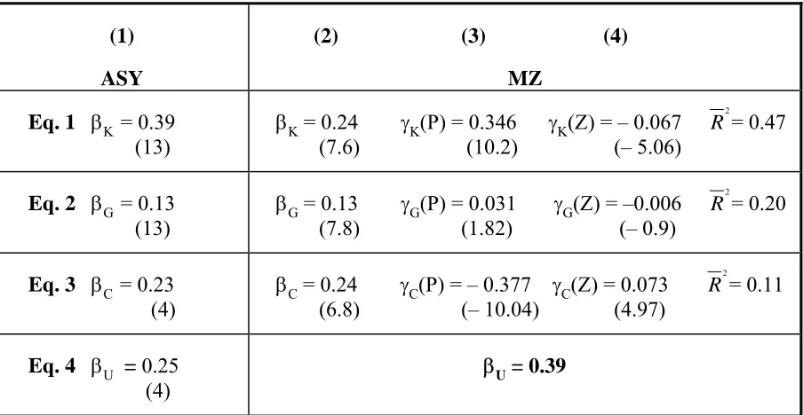
Mélitz and Zumer (1999) offer some relevant evidence. Table 3 shows ASY’s aforementioned

estimates of βK, βG,βC and βU in the first column. These estimates rest on pooling of

equa-tions (7) and generalized least squares. The next three columns provide revised estimates by

Mélitz and Zumer (MZ) based on the identical data. There are four notable differences. First,

instead of time fixed-effects, MZ use ratios of regional values to national values to correct for

movements in the aggregates. Second, they add regional fixed effects (to allow for possible

drift or trend in regional ratios). Thus, the equations are not the same. Nevertheless, these first

two departures yield no difference of note in estimates for the U.S. Third, MZ suppose βU

equal to 0.39, as mentioned before. Consequently, they estimate only the first three of the

equations (7) as a system, and impose the cross-equation restriction βK + βG +βC = 1–0.39.

Last, and most relevant at present, they add a few variables to reflect influences that condition

the effects of the regional output shocks. (Conformably, they impose a separate

cross-equation restriction requiring the trio of coefficients associated with each of the influences to

sum to zero, so that the restriction βK + βG +βC = 1–0.39 still remains the right one.) The table

reports the results concerning two of the extra influences: the Campbell-Mankiw index of

persistence of the asymmetric shocks (P); and the degree of asymmetry of the individual-state

business cycle (Z) (as inferred with the use of a Hodrick-Prescott filter).6 _{The results relating}

to Z, or the smoothing of short run shocks, imply some offsetting behavior by households in

response to dividends policy. Therefore, these results confirm the possibility that ASY

over-estimate βK and the smoothing by firms. But this requires some explanation.

The last column in Table 3 (concerning Z) shows that in the event that shocks reflected

strictly the (state-specific) business cycle, household saving would explain 7 percent more of

the smoothing (7 percent less would be done by firms). This in itself could simply issue from

the fact that the only uninsured shocks that households are able to smooth through credit are

transitory ones (ASY’s interpretation). But as is not directly inferable from the table, omitting

the variable Z from the analysis also raises βK relative to βC by the full 7 percent. In other

words, the failure to isolate short run influences in any way leads to a greater attribution of

smoothing to firms relative to households. That suggests more: namely, the earlier

6 _{The estimated system is:}

iK i i ,j j , K i K K i

i logpi logy (logX ) logy

y

log −∆ =α +β ∆ +γ ∆ +µ

∆ iG i i ,j j , G i G G i

i logdi logy (logX ) logy

pi

log −∆ =α +β ∆ +γ ∆ +µ

∆ (5)

iC i i ,j j , C i C C i

i logc logy (logX ) logy

di

log −∆ =α +β ∆ +γ ∆ +µ ∆

subject to β_K+β_G+β_C= −1 β_U, 0<β_U<1 and for all j, j=1,...,n, γ_{K j,} +γ_{G j,} +γ_{C j,} =0

where the Xj variables are new influences in the econometric analysis. The use of lower-case

letters instead of the upper-case ones in equations (7) serves to indicate that the variables are no longer per capita values, as before, but ratios of per capita values to per capita national averages (adding up to one with appropriate weights). Table 3 only reports the results for P and Z, but there are two other Xj variables in the study.

tion: that households offset some unnecessary smoothing of shocks by firms via dividends

policy.7

As seen by comparing columns 1 and 2, the sum outcome of MZ’s revisions is to lower βK

and to keep βG and βC unchanged. Because of these changes, the regional smoothing of

shocks via adjustments in the income households receive from firms no longer seems larger

than the regional smoothing of shocks via household saving.

In short, two basic conclusions emerge: first, ASY exaggerate the extent of risk sharing;

sec-ond, they ascribe too much of the smoothing of output shocks to portfolio diversification and

to firms and too little to household saving. In the international application, further doubts will

set in about the proper measure of risk-sharing via credit as such.

III. Risk-sharing via credit and cross-ownership of property in the EMU

In the case of international evidence, ASY’s method becomes easier to apply. The data are

superior. ASY even needed to infer consumption by individual state in the U.S. from retail

sales. On the international front, the national accounts provide the required series for

con-sumption. Moreover, the current account statistics offer figures for net foreign lending or the

accumulation of claims on foreigners. In addition, the difference between gross national

product and gross domestic product yields net income on foreign property claims.

Accord-ingly, we can begin from the following identity:

Y Y GNP

GNP A

A C C

i i

i i i

i i

i

= (8)

where Yi is gross domestic product (as before), GNPi is gross national product, Ai is home

7 _{With respect to P, column 3 shows, in conformity with earlier discussion, that if all the}

shocks were persistent, the smoothing via business saving would be about 35 percent greater. However, very significantly, removing P, and thus treating all shocks indifferently without regard to degree of persistence, does not affect the respective estimates of βK and βC. There is

therefore no evidence that households offset the smoothing of persistent shocks by firms. In terms of Modigliani-Miller, this means that the smoothing of persistent shocks via business saving may reflect optimal policy and may be in the shareholders’ best interests. If so, the households would have no cause to offset the smoothing of the permanent shocks by firms.

absorption, Yi − Ai is therefore the export surplus on current account, and finally, Ci is the

sum of private and public consumption. Proceeding as ASY did before, we then have:

iK i 1 K K i

i logGNP logY

Y

log −∆ =α +β ∆ +µ

∆ iC i 1 C C i

i logA logY

GNP

log −∆ =α +β ∆ +µ

∆ (9)

iS i S

S i

i logC logY

A

log −∆ =α +β ∆ +µ ∆

∆logC_i =α_U+β_U∆logY_i +µ_iU

In this case, βK1 concerns much more precisely what ASY intended before by βK, and the

same may be said for βC1 with regard to βC. But, of course, a separate term must enter, βS,

relating to smoothing of output shocks via strict domestic saving, some of it by firms, some of

it by households. There is one basic qualification to this general idea of the superiority of

equations (9) to equations (7) in analyzing risk-sharing. The differences between GDP and

GNP may cover income flows, but they do leave out capital gains and losses on international

claims. Therefore, any smoothing of output shocks that would be associated with such gains

and losses would not enter in βK1, where in principle it belongs. It would affect βS instead. In

addition, equations (9), as they are now stated, ignore any term for βG, thus any role for

stabi-lization by a super-government. True, the EU Commission has a budget, but it is small in

rela-tion to GDP, and the EU structural funds program relates essentially to redistriburela-tion rather

than stabilization.

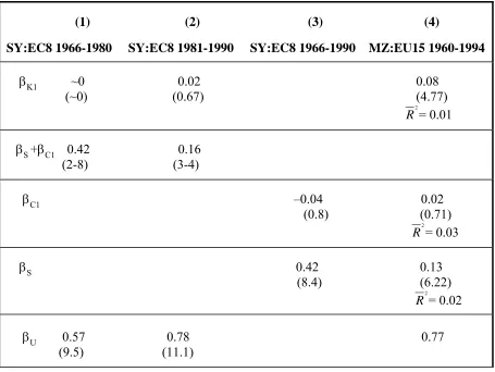
Table 4 provides estimates of equations (9). In this case, the sources are Sørensen and Yosha

(1998) (hereafter SY) and MZ. In both instances, the table reports the results relating most

closely to the current EMU members: namely, the EU8 (Belgium, Denmark, France,

Ger-many, Ireland, Italy, the Netherlands and the UK) in the case of SY and the EU15 in the case

of MZ. In both cases, the reported results also cover the period that compares best with the

one in ASY (1964 to 1990). Like ASY, SY estimate βU by running the last of the regressions

in equations (9) while MZ impose βU based on the same ratio of variances as was noted

be-fore in discussing their work (footnote 4). SY also deal with βC1 strictly in the context of a

separate decomposition of βS + βC1. For SY, 22 to 43 percent of the asymmetric output shocks

are smoothed; for MZ only 23 percent. For SY, the smoothing is entirely domestic, and there

is no risk-sharing. For MZ, there is some risk-sharing, 8 percent, coming from the

cross-ownership of claims to property, but most of the smoothing is domestic. In both studies,

cur-rent account balances explain nothing: there is no international smoothing of asymmetric

shocks via credit.

These results about risk-sharing may seem reasonable on the surface. We would not expect

much crosscountry insurance against asymmetric shocks in light of the importance of home

preference in portfolios of equities. Ratios of foreign direct investment to total home

invest-ment are also generally small. Even MZ’s estimate of 8 percent for insurance via international

portfolio diversification may look high. In addition, the Feldstein-Horioka puzzle speaks

pre-cisely about the small contribution of foreign saving to the financing of domestic investment.

Correlations between domestic saving and domestic investment (both as percentages of GDP)

over periods of five to seven years or over are much higher than we would expect under

per-fect risk sharing. Feldstein and Horioka (1980) found those correlations to be close to one in

the OECD in their initial study, covering the 60s to mid-70s. The correlations have dropped

since. But as Obstfeld and Rogoff (2000) stress, the correlations are still 60 percent in the

OECD over 1990-97; and nothing resembling similarly high numbers exists in corresponding

studies of regions within countries (Helliwell (1998)). Thus, it seems reasonable too that βC1

would be negligible in table 4.

However, there are other sources of evidence about risk-sharing in the EMU. The system now

exists since 1999. What are the other indications thus far?

I cannot pretend to do justice to the question. That would require a separate study. One

vol-ume of the recent report of the British Treasury (2003) about entry into EMU, titled EMU and

the cost of capital, provides a summary of the evidence. Some increase in the diversification

of equity portfolios has occurred in the membership since the run-up to EMU. Cross-country

correlations between returns on equities have risen. The total variance of equity returns in the

EMU now seems to depend less on country-specific factors and more on common industry

factors. There have also been a number of cross-country mergers and acquisitions, though

fewer than expected. To all evidence, though, as regards the diversification of property

claims, the EMU still has a long way to go before approaching the degree of capital market

integration in the U.S.

On the other hand, with respect to the availability of credit from the rest of the membership,

the closing of the gap between the euro zone and the US has gone very far. The bond market

in euros took off as soon as it appeared. Gross international issues of bonds and notes in euros

just about tripled between the end of 1997 and the end of 1999 (H.M. Treasury (2002), chart

4.1), as compared with issues in predecessor currencies. Before the appearance of the euro,

bond issues by firms and public agencies in the euro zone had been predominantly triple A

and double A (80 percent of them as late as 1998). Since then, single A and triple B issues

have become a high percentage of the total: over 40% in 2001 (ibid. table 4.1). Evidently,

numerous borrowers in the euro zone who had previously relied exclusively on banks now

issue bonds in euros. Holdings of bonds of the major governments in the euro zone are also

now widely held in the membership and internationally. Most significant of all perhaps, little

remains of the Feldstein-Horioka puzzle. Blanchard and Giavazzi (2002) report a value of

0.14 for the relevant coefficient in the regression for domestic investment for the euro area

over 1991-2001, down from 0.41 in 1975-1990. In addition, the current account deficits of the

two present members of EMU who are still in a catch-up phase, Portugal and Greece, rose to

10 and 6-7 percent of GDP, respectively, in 2000-2001.

How much more smoothing of asymmetric shocks has already come from this rapprochement

with the U.S. in the euro zone and how much is still to follow? The very nature of the

ques-tion is important: it poses the matter differently than we encountered it before. The issue is

not how much of the risk-sharing already results or will result in the future from credit, but by

how much credit already reduces or will reduce the fraction of the shocks that remain

unsmoothed. We might think that we should get roughly the same answer either way. If a

mechanism accounts for a particular percentage of the smoothing, its absence should reduce

the smoothing as much. As regards risk sharing through property claims, Athanasoulis and

van Wincoop (2001)’s results go in this direction. These authors, in fact, approach the issue

of insurance (or risk-sharing via asset diversification) precisely from the angle of a reduction

in βU. Despite some difference in their measure of βU (in the same spirit as the one in MZ)

and despite their strict focus on the long-term horizon (to eliminate transitory shocks), they

get analogous figures for βK in the U.S. (and for βG too for that matter) to those in ASY.8 But

as regards risk-sharing through credit, some reflection will show that a focus on the negative

impact on βU is almost bound to make a difference: the very sign of βC1 is ambiguous.

In reasoning about βC, in fact, ASY reason strictly about βC1, since their analysis relates

strictly to borrowing and lending. They conclude that the sign must be positive because a

permanent asymmetric shock to output should have no effect on lending or borrowing,

whereas a transitory one should raise lending if the shock is positive and borrowing if the

shock is negative. Thus, in case of a mix of permanent and transitory shocks, positive values

follow for βC1. However, the examples of Portugal and Greece reveal the precariousness of

this reasoning. Suppose that a positive permanent shock implies a rising profile of output in

the future (catch-up). Then the country ought to borrow and βC1 can be expected to be

nega-tive. There is also a major difficulty in regard to transitory shocks. Assume a recession. The

affected country should save less, or in terms of SY, the sign of βS should be positive.

How-ever, imports will fall with the drop in income, and may do so more than exports (which

might have dropped under the initial impact of the shock). Indeed, if the shock lowers the

terms of trade enough and shifts demand sufficiently in favor of home goods, then a fall in

imports minus exports is to be expected. Once again, the sign of βC1 will be negative. This

last example actually fits well with usual macroeconomic modeling – better than ASY’s logic

8 _{Their estimates vary from 0.35, almost exactly ASY’s figure, to 0.215, close to MZ’s,}

de-pending on the presence (0.35) or absence (0.215) of interest and dividends in personal in-come. Athanasoulis and van Wincoop (2001) also consider those figures to pertain strictly to regional insurance, or βK1 rather than βK. In so doing, though, they disregard the fact that

many firms are owned entirely by state residents and operate strictly within state borders. These firms’ saving behavior would affect their estimate but have nothing to do with insur-ance and the sharing of risks between states.

in favor of a positive sign for βC1. Our models often say that recession yields a short run

im-provement in the current account balance in light of the size of the fall in imports. Thus,

re-gardless whether shocks are permanent or transitory, the sign of βC1 is ambiguous.9

In sum, it is already a live issue today to know how much extra risk-sharing there is and how

much is still to arrive in the euro area because of greater ease of borrowing and lending. But

unfortunately, ASY, SY and MZ offer little guidance. Their method of investigation will not

allow us to answer the question.

IV. The impact of EMU on total insurable risks

Discussion of EMU often focuses on the degree to which shocks are symmetric. In the present

context, this concerns the extent to which the risks are insurable by the market. So far as risks

are common and cannot be insured, of course, they can be managed through joint monetary

policy. This is the usual emphasis. But it is important to consider the issue of the extent of

common risks from the perspective of the potential for risk-sharing through market channels

as well.

A frequent starting point is Krugman’s (1991, 1993) prediction that EMU would lead to more

region-specific shocks and thereby less scope for smoothing shocks through monetary policy.

According to his assessment, the U.S. regions are more specialized than the EMU countries of

comparable size, probably because of the closer approximation to a single market in the U.S.

Hence, as impediments to trade diminish and capital markets become more integrated in the

EMU, the members can expect to move toward greater industrial specialization. These

coun-tries will then experience increasing asymmetry of shocks.

9 _{In both of the previous examples of a negative sign of} β_{C1, credit is also likely to smooth}

consumption and therefore to reduce βU. This is capital. In the example of a permanent shock

yielding a rising profile of output over time, the borrowing permits a smaller upward tilt in consumption. In that of the adverse transitory shock, the lending abroad moderates the drop in output, and thereby may cushion the fall in current consumption. Repairing the problem in ASY’s analysis in the latter case, pertaining to the transitory shock, would clearly mean re-moving their identification of the exogenous shock with the observed change in output.

Subsequent empirical investigation does not particularly agree with Krugman’s analysis. He

had compared U.S. data for 1977 with European data for 1985. But Kim (1995) shows that

the trend in the U.S. has been going the other way for years beforehand: “regional

specializa-tion … fell substantially and continuously between the 1930s and 1987” (p.882).10 _According

to Peri (1998), by 1986, regional specialization was already no higher in the U.S. than in the

EU. Furthermore, Clark and van Wincoop (2001) report lower or equal specialization in the

eight census regions of the U.S. than in the EU14 over 1981-1997.

Recent empirical work on the symmetry of business cycles sheds further doubt on Krugman’s

views. To go back a bit, test results indicate that monetary union promotes bilateral trade

(Rose (2000)). Conformably, Micco, Stein and Ordoñez (2003)) show that EMU has already

brought a certain increase in bilateral trade since 1998. In addition, Frankel and Rose (1998)

display a tendency for business cycle correlations to rise with the intensity of bilateral trade in

the OECD. Still more recent research by Engel and Rose (2003) and Clark and van Wincoop

(2001) corroborates Frankel and Rose’s results, in the case of the former based on a

world-wide sample of countries, in the case of the latter, based on a narrower sample of countries

and regions in the OECD. Taken together with the Rose evidence, the inference would be that

EMU will tend to promote the symmetry of business cycles.

Studies by Firdmuc (2004) and Kalemli-Ozcan, Sørensen and Yosha (2001) are relevant too.

Firdmuc (2004) offers econometric evidence that intra-industrial trade raises symmetry of

business cycles, while inter-industrial trade does the opposite. This would imply that the

pre-vious evidence of the rise in the symmetry of business cycles with increasing trade reflects the

influence of intra-industry trade. For their part, Kalemli-Ozcan, Sørensen and Yosha (2001)

provide indications that industrial specialization reduces the symmetry of business cycles.

This is true both for regions within countries and between countries. These three authors’

10 _{Evidently aware of this evolution, Krugman (1993) put the evidence in doubt. See his note}

4.

sult would seem to support Krugman’s general intuition. But if we link the result to the

evi-dence that greater bilateral trade increases the correlation of business cycles, the implication

would be that with greater trade, regions and countries become less specialized.11

There is no difficulty explaining why EMU would promote intra-industry trade, reduce

na-tional specialization, and increase the symmetry of business cycles. As income rises, the new

trade may well predominantly concern goods that are highly income-elastic and price-elastic

in demand. This means more trade in differentiated products and increasing intra-industry

trade. If the same industries take foot everywhere, countries become less specialized.12 _The

rise in the symmetry of business cycles with advancing intra-industry trade can follow in

many ways. As intra-industry trade goes forward, industry shocks will become increasingly

common shocks. With greater market integration, all shocks may also spread more quickly, as

Frankel and Rose (1998) stress, and this can raise the covariance of aggregate business

activ-ity.

Notwithstanding, the previous evidence does raise a certain difficulty of interpretation.

Ac-cording to standard microeconomic analysis, individuals should be willing to bear more

pro-duction risks as capital market integration deepens. They can insure themselves better; and

they can borrow more easily. Hence, production risks should be less of a concern to them.

Based on a large literature, insurance opportunities encourage people to accept riskier, higher

return projects. (See, among many others, Obstfeld (1994) and Kalemli-Ozcan, Sørensen and

Yosha (1999, 2001).) How then do we reconcile this theoretical argument with a tendency of

EMU to lead toward higher symmetry of business cycles? Does such a tendency fly in the

face of theory?

There are two avenues of reconciliation. One is to ascribe the recent increase in symmetry of

11 _{Kalemli-Ozcan, Sørensen and Yosha’s own emphasis differs distinctly.}

12 _{But the diminished national specialization need not signify diminished regional}

specializa-tion, since with a reduction in some border costs – say, multiple money ones – but not others, firms may move their production closer to their neighbors without traversing frontiers.

business cycles to low capital market integration, low international insurance, and limited

international credit. On this view, as capital market integration advances and people pool their

risks more efficiently and obtain larger, more secure lines of credit, they will undertake riskier

output projects. Then the asymmetry of shocks in the euro zone will increase. Of course, this

will also expose uninsured workers in the euro zone to an increasing share of the risks. It will

therefore raise the urgency of increasing the flexibility of the labor market. The lack of any

system of transfer payments through upper-level government in the EMU will also possibly

become an increasing handicap. This line of reasoning evidently tends to take us back to

Krugman’s views and may underlie the appeal of his stand.

The other avenue of reconciliation is to argue that the euro has indeed already led to an

in-crease in production risks. But the new risks are common, and therefore consistent with

greater symmetry of business cycles. On this next view, there has been notable progress in

capital market integration in the euro zone. But the move to a more efficient allocation of

risks has not meant moving to greater specialization of output activities within national

fron-tiers. Presumably, in this case, the new technologies simply do not require notable increase in

individual plant size. Since the added risks are common, they are manageable through joint

macroeconomic policy. Of course, if so, the burden of responsibility on the European Central

Bank also rises. Consequently, greater flexibility of labor markets still helps, and may help a

lot, in attenuating shocks. But macroeconomic policy at the EU level has a larger role to play

in smoothing economic activity.

Evidently, the second view is far more optimistic. If the first view is right, then the euro zone

has not advanced much toward an efficient allocation of risks. Instead, the zone has largely

sought shelter against the winds of competition through increasing diversification at home.

Not only does this limit welfare, but market forces will tend to work in the future toward a

change in direction: that is, a move toward greater specialization on a national basis. The

zone will then eventually need to face the associated problem of inability to extend market

insurance to labor.

TABLE 1

STABILIZATION AND REDISTRIBUTION VIA FEDERAL TRANSFERS IN THE

U.S. 1977-1992: 48 REGIONS

STABILIZATION

Level: eq. (1) First difference: eq. (2)

REDISTRIBUTION

Eq. (3)

1–βs R

2

1–βs R

2

1–βd R

2

PERSONAL

INCOME

0.272 0.922 (0.008)

0.20 0.846 (0.012)

0.213 0.974 (0.019)

GROSS

PRODUCT

0.13 0.985 (0.004)

0.118 0.968 (0.006)

0.136 0.976 (0.02)

The standard errors in parentheses pertain to βd or to βs. Regional constants are omitted. Net

transfers consist of direct taxes and social insurance, transfers to persons and federal grants to state and municipal governments. See Mélitz and Zumer (2002).

TABLE 2

STABILIZATION AND REDISTRIBUTION VIA FEDERAL TRANSFERS IN THE

U.S. 1977-1992: 48 REGIONS

STABILIZATION: PERSONAL INCOME

Level First difference Eq.(1) Eq. (2)

STABILIZATION: GROSS PRODUCT

Level First difference Eq.(1) (Eq. (2)

NET

TRANSFERS

1–βs R2 1–βs R2 1–βs R2 1–βs R2

(1) DIRECT TAXES AND SOCIAL INSURANCE 0.086 (0.007) 0.977 0.063 (0.012) 0.898 0.03 (0.003) 0.998 0.031 (0.006) 0.979

(2) DIRECT TAXES, SOCIAL INSURANCE, AND TRANSFERS TO PERSONS

0.234

(0.007)

0.941 0.149

(0.012)

0.878 _0.097

(0.003)

0.99 0.089

(0.006)

0.974

(3) DIRECT TAXES, SOCIAL INSURANCE, TRANSFERS TO PERSONS AND GRANTS 0.272 (0.008)

0.922 0.20 (0.012)

0.846 _0.13

(0.004)

0.985 0.118

(0.006) 0.968

REDISTRIBUTION: PERSONAL INCOME Eq. (3) REDISTRIBUTION: GROSS PRODUCT Eq. (3) NET TRANSFERS

1–βd R2 1–βd R2

(1) DIRECT TAXES AND SOCIAL INSURANCE

0.0863

(0.009) 0.996

0.04 (0.021)

0.98

(2) DIRECT TAXES, SOCIAL INSURANCE, AND TRANSFERS TO PERSONS

0.181

(0.016) 0.982

0.124

(0.016) 0.984

(3) DIRECT TAXES, SOCIAL INSURANCE, TRANSFERS TO PERSONS AND GRANTS

0.213

(0.019) 0.974

0.136

(0.004) 0.976

The standard errors in parentheses pertain to βd or to βs. See Mélitz and Zumer (2002).

TABLE 3

ESTIMATES OF THE ASY (ASDRUBALI-SØRENSEN-YOSHA) AND THE REVISED ASY MODEL

USA 1964-1990

(1)

ASY

(2) (3) (4)

MZ

Eq. 1 β_K = 0.39 (13)

β_K = 0.24 γ_K(P) = 0.346 γ_K(Z) = – 0.067 R2= 0.47 (7.6) (10.2) (– 5.06)

Eq. 2 β_G = 0.13

(13)

β_G = 0.13 γ_G(P) = 0.031 γ_G(Z) = –0.006 R2= 0.20 (7.8) (1.82) (– 0.9)

Eq. 3 β_C = 0.23

(4)

β_C = 0.24 γ_C(P) = – 0.377 γ_C(Z) = 0.073 R2= 0.11 (6.8) (– 10.04) (4.97)

Eq. 4 β_U = 0.25 (4)

β_U = 0.39

Sources: Asdrubali, Sørensen and Yosha (1996); Mélitz and Zumer (1999). Student t’s are in parentheses, as in the original ASY article. For the interpretation of γ_K(P) and γ_K(Z), see foot-note 6 and the associated text.

TABLE 4

ESTIMATES OF THE ASY MODEL BASED ON INTERNATIONAL EVIDENCE

(1) (2) (3) (4)

SY:EC8 1966-1980 SY:EC8 1981-1990 SY:EC8 1966-1990 MZ:EU15 1960-1994

β_K1 ~0 0.02 0.08

(~0) (0.67) (4.77) R2= 0.01

β_S +β_C1 0.42 0.16

(2-8) (3-4)

β_C1 –0.04 0.02

(0.8) (0.71) R2= 0.03

β_S 0.42 0.13

(8.4) (6.22) R2= 0.02

β_U 0.57 0.78 0.77 (9.5) (11.1)

Notes: The sources are Sørensen and Yosha (1998) and Mélitz and Zumer (1999). The EC8 in columns 1 and 2 refer to Belgium, Denmark, France, Germany, Ireland, Italy, the Netherlands and the UK. The first two columns come from Sørensen and Yosha’s Table 1. β_K1 refers to their β_f, and β_S +β_C1 to their β_d and β_s combined. Column 3 comes from their Table 6. Column 4 relates to Mélitz and Zumer, table 10 (where β_S is denoted β_K2). Student t’s are in paren-theses.

REFERENCES CITED

Asdrubali, Pierfederico, Bent Sørensen and Oved Yosha (1996). "Channels of inter-state risk-sharing: United States 1963-1990," Quarterly Journal of Economics, 111, pp. 1081-1110.

Athanasoulis, Stefano and Eric van Wincoop (2001). "Risksharing within the United States: What have financial markets and fiscal federalism accomplished?" Review of Econom-ics and StatistEconom-ics, 83, pp. 688-698.

Bayoumi, Tamim and Paul Masson (1995). "Fiscal flows in the United States and Canada: Lessons for Monetary Union in Europe," European Economic Review, 30, pp. 253-274.

Blanchard, Olivier and Lawrence Katz (1992). “Regional evolutions,” Brookings Papers on Economic Activity, no. 1, pp. 1-75

Blanchard, Olivier and Francesco Giavazzi (2002). “Current account deficits in the euro area: The end of the Feldstein-Horioka puzzle?” Brookings Papers on Economic Activity, no. 2, pp. 147-209.

Campbell, John and Gregory Mankiw (1987). "Are output fluctuations transitory?" Quarterly Journal of Economics, 102, pp. 857-880.

Clark, Todd and Eric van Wincoop (2001). “Borders and business cycles,” Journal of Inter-national Economics, 55, pp. 59-85.

Decressin, Jörg (2002). “Regional income redistribution and risk sharing: how does Italy compare in Europe?” Journal of Public Economics, 86, pp. 287-306.

Del Negro, Marco (2002). "Asymmetric shocks among U.S. states," Journal of International Economics, 56, pp. 273-297.

Engel, Charles and Andrew Rose (2003). “Currency unions and international integration,” Journal of Money, Credit and Banking 34, pp. 804-826.

Feldstein, Martin and Charles Horioka (1980). "Domestic saving and international capital flows," Economic Journal, 90, pp. 314-329.

Fidrmuc, Jarko (2004). “The endogeneity of the optimum currency area criteria and intra-industry trade: implications for EMU enlargement,” in Paul De Grauwe and Jacques Mélitz, eds., Monetary Unions after EMU, MIT Press, forthcoming.

Frankel, Jeffrey and Andrew Rose (1998). "The endogeneity of the optimum currency area criteria" Economic Journal, 108, pp. 1009-1025.

Goodhart, Charles and Stephen Smith (1993). "Stabilisation," in EC, "The Economics of Community Public Finance," European Economy, Reports and Studies, 5, pp. 417-55.

Helliwell, John (1998). How Much do National Borders Matter? Washington, D.C.: Brook-ings Institution.

Hess, Gregory and Eric van Wincoop (2000). International Macroeconomics, Cambridge University Press.

HM Treasury (2003). EMU and the Cost of Capital: EMU Study.

Kalemli-Ozcan, Sebnem, Bent Sørensen and Oved Yosha (1999). “Risk sharing and industrial specialization: regional and international evidence,” working paper, University of Hous-ton, Federal Reserve Bank of Kansas City and Tel Aviv University.

Kalemli-Ozcan, Sebnem, Bent Sørensen and Oved Yosha (2001). “Economic integration, industrial specialization, and the asymmetry of macroeconomic fluctuations,” Journal of International Economics, 55, pp. 107-137.

Kim, Sukko (1995). “Expansion of markets and the geographic distribution of economic ac-tivities: the trends in U.S. regional manufacturing structure, 1860-1987,” Quarterly Journal of Economics, 110, pp. 881-908.

Krugman, Paul (1991). Geography and Trade, MIT Press.

Krugman, Paul (1993). "Lessons of Massachusetts for EMU," in Francisco Torres and Fran-cesco Giavazzi, eds. Adjustment and Growth in the European Monetary Union, Cam-bridge University Press, pp.241-261.

Mélitz, Jacques and Frédéric Zumer (1999). "Interregional and International Risk Sharing and Lessons for EMU," Carnegie-Rochester Conference Series on Public Policy, vol. 51, pp. 149-188.

Mélitz, Jacques and Frédéric Zumer (2002). "Regional redistribution and stabilization by the center in Canada, France, the United Kingdom and the United States: A reassessment and new tests," Journal of Public Economics, 86, pp. 263-286.

Micco, Alejandro, Ernesto Stein and Guillermo Ordoñez (2003). “The currency union effect on trade: early evidence from EMU,” Economic Policy , 37, pp. 317-356.

Obstfeld, Maurice (1994) "Risk-taking, global diversification and growth,” American Eco-nomic Review, 84, pp. 1310-1329.

Obstfeld, Maurice and Giovanni Peri (1998). "Regional Nonadjustment and Fiscal Policy," Economic Policy, 26, April, pp. 205-59.

Obstfeld, Maurice and Kenneth Rogoff (2000). “The six major puzzles in international mac-roeconomics: Is there a common cause?” In Ben Bernanke and Kenneth Rogoff, eds., NBER Macroeconomics Annual 2000, pp. 339-390.

Peri, Giovanni (1998). “Technological growth and economic geography,” mimeo., Bocconi University.

Andrew Rose (2000). “One money, one market: Estimating the effects of common currencies on trade,” Economic Policy, pp. 7-46.