Simulation of a model-based optimal controller for heating systems under realistic hypothesis

SIMULATION OF A MODEL-BASED OPTIMAL CONTROLLER FOR HEATING

SYSTEMS UNDER REALISTIC HYPOTHESES

Michaël Kummert

and Philippe André

1

_{École Polytechnique de Montréal, Dépt. de Génie Mécanique}

Case Postale 6079, succursale Centre-Ville, Montréal, QC H3C 3A7, Canada

michael.kummert

polymtl.ca

2

_{Université de Liège, Dépt. des Sciences et Gestion de l'Environnement – Arlon, Belgium}

ABSTRACT

An optimal controller for auxiliary heating of passive solar buildings and commercial buildings with high internal gains is tested in simulation. Some of the most restrictive simplifications that were used in previous studies of that controller (Kummert et al., 2001) are lifted: the controller is applied to a multizone building, and a detailed model is used for the HVAC system. The model-based control algorithm is not modified. It is based on a simplified internal model.

It is shown that the optimal controller's performance varies strongly with the zone that is considered and the reference zone that is used. However, it is never worse than the performance of a reference controller. The global performance at the building level depends on the selected reference zone and on the building sensitivity to overheating.

INTRODUCTION

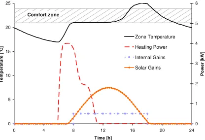
The problem of heating control in passive solar buildings or in modern, well-insulated buildings with high internal and/or solar gains, is characterized by a need of anticipation, which is illustrated in Figure 1.

0 5 10 15 20 25

0 4 8 12 16 20 24

Time [h]

Te

mp

er

a

tu

re [

°C]

0 1 2 3 4 5 6

Po

we

r [

k

W]

Zone Temperature Heating Power Internal Gains Solar Gains

Comfort zone

Figure 1: Typical building behavior, sunny mid-season day

If there is no cooling plant, overheating can occur during a sunny afternoon while heating was necessary in the morning. In this case, when overheating occurs, it is too late to take a control decision for the heating plant: the heat stored in the building structure cannot be removed. If a cooling

plant was present, the temperature could be maintained in the comfort zone in the afternoon, but this would increase the electricity load during on-peak hours. If afternoon overheating is anticipated, it is possible to reduce heating in the morning, saving heating energy and improving thermal comfort (or reduce cooling cost) at the same time.

Estimating the recovery time after night setback is another example where anticipation is required. Energy savings can be realized by applying an important setback and by warming-up the building as late as possible, but enough warm-up time must be given to prevent occupant complaints if the building is too cold. This situation expresses the permanent search for a compromise between energy concerns (low temperature during night, heating started as late as possible) and comfort concerns (warm building when occupants arrive).

The observations here above justify the interest for predictive optimal controllers in passive solar buildings.

LITERATURE SURVEY

Optimal control studies related to buildings can be subdivided in two categories: auxiliary heating (and sometimes cooling) control in solar buildings, and cooling system optimization. The first category finds its origin in the need for anticipation illustrated here above, while the second typically allows important savings in terms of money because optimal control can take advantage of time-of-day electricity rates. Some cooling optimization studies only address the cooling plant operation – in that case building loads are fixed and comfort is not part of the equation (Flake, 1998). This is also true for most studies on ice storage optimization where building loads have to be anticipated but where they are considered to be independent from the controller actions (Henze et al., 1997). Other studies (e.g. Keeney and Braun, 1996) consider the comfort issue as boundaries that must not be exceeded and optimize the operation of the cooling system in order to maintain the building at the desired setpoint.

significant savings compared to reference controllers (Nygard-Fergusson, 1990; Oestreicher et al., 1996). In both types of studies, the concept of reference zone is very often used (Braun, 1990): The controller optimizes the energy consumption while maintaining comfort in a reference zone. Most advanced controllers implement a model-based predictive strategy, which implies that they are based on an internal model of the system (building and/or HVAC plant). In simulation studies, the model that is used in the (detailed) simulation can be the same as the controller's internal model. However, it has been shown that the simulated performance of optimal controllers deteriorates when more detailed models are used to assess their performance (Kummert et al., 1996).

OBJECTIVE OF THIS STUDY

The present study aims at assessing the performance of an optimal controller developed to optimize the behavior of one reference thermal zone based on a simplified internal model. The performance at the building level is assessed using detailed models for the building and the HVAC system.

OPTIMAL CONTROL ALGORITHM

The principle of model-based predictive control is to use a model of the system and a forecast of future disturbances to simulate possible future control sequences and select the "best" one over a given forecasting horizon. This controller is also optimal in the sense that it minimizes a given cost function taking discomfort and energy use into account. The cost function is described in the "Performance Criterion" section.

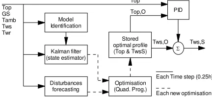
Figure 2 shows the implemented optimal controller (Kummert, 2001). The control algorithm was developed in Matlab (The Mathworks, 1999), which was then called from TRNSYS. Its principle is briefly described here under.

1. At each time step (0.25h) some variables are measured: zone operative temperature (Top),

radiator supply and return temperature (respectively Tws and Twr), ambient temperature

(Tamb) and solar radiation on southern façade

(GS).

2. These variables are passed to three different subsystems:

- A system identification routine that adapts the parameters of the controller's internal model using the latest available measurements. The internal model is described in the next Section. - A Kalman Filter (State estimator), which

estimates the state of the internal model. This provides the initial conditions for the optimization.

- A disturbance forecasting algorithm that predicts the ambient temperature and solar radiation for the next optimization period (e.g. 24 h). In this study the forecasting algorithm was just repeating the data from previous day.

3. At the beginning of each new optimization period, the optimization algorithm minimizes the cost function on the given horizon (NH hours). It

outputs an "optimal" 0.25h-profile of Top and Tws

(respectively Top,O and Tws,O). The optimization

uses the estimated state of the system, the newly identified parameters and the disturbance forecasting to simulate the next NH hours and

select the best future control sequence. The optimization uses a quadratic programming algorithm (Quad. Prog. in Figure 2).

4. After the optimal profile has been computed, the desired zone temperature profile is known (Top,O).

If the model and the disturbance forecast were perfect, that temperature would be obtained by providing a water supply temperature that matches the calculated profile (Tws,O). A PID is

cascaded with the optimal controller to compensate for modeling and forecasting errors. The PID tracks the setpoint for Top (i.e. Top,O). Its

output adjusts the setpoint for the water supply temperature (Tws,S).

Disturbances forecasting Kalman filter (state estimator)

Model Identification

Optimisation (Quad. Prog.) Stored optimal profile (Top & TwsS)

PID

Tws,O Top,O Top

Tws,S

Each Time step (0.25h)

Each new optimisation

Σ

Top GSouth Tamb Tws Twr

Figure 2: Optimal controller block scheme

CONTROLLER'S INTERNAL MODEL

The controller is based on a simplified model of the building and the HVAC system. This model is a key component of the controller, because it allows simulating future control sequences to select the optimal one. This internal model has to be simplified in order to keep the optimization algorithm computationally efficient.

(e.g. ambient temperature or adjacent zones). Ventilation is modeled through an additional flow path between the zone air temperature and the ambient temperature, with a resistance adjusted to match the outside air flowrate. Humidity is not taken into account in the controller's internal model. The radiator is modeled as a single node and heat emission characteristics are linearized. The average between the radiator temperature (which is assumed to be equal to Twr) and the water supply temperature

(Tws) is used to compute the power emission. Heat

flux is directed to air and to wall surfaces according to a fixed ratio. The simplified model only takes into account the inertia and the maximal power of the boiler (a constant efficiency is assumed), and pipes are neglected.

PERFORMANCE CRITERION

The notion of "cost function" is used to assess the performance of different controllers. The cost function must be an expression of the trade-off between comfort and energy consumption. The chosen indicator of thermal (dis)comfort is Fanger's PPD (Predicted Percentage of Dissatisfied – Fanger, 1972), while energy cost is considered to be proportional to the boiler energy consumption (Qb).

In the discomfort cost, Fanger's PPD is computed with default parameters for non-simulated aspects (air velocity and metabolic activity). Furthermore, it is assumed that occupants can adapt their clothing to the zone temperature. This method allows modeling a comfort range in which occupants are satisfied. With the chosen value for parameters, the comfort zone covers operative temperatures from 21°C to 24°C. The PPD is also shifted down by 5%, to give a minimum value of 0. This modified PPD index will be referred to as PPD'.

This gives, respectively for discomfort cost and energy cost (Jd and Je):

(

)

d

J =

∫

e b

J =

∫

The total cost (J) is a weighted sum of Jd and Je:

d e

J= αJ +J (3)

The role of the α parameter is to give more or less importance to comfort with respect to energy. It can be seen as a "comfort setting" of the controller. If a user increases the value of α, she/he is actually saying that comfort should have more importance in the trade-off that is made to control the HVAC plant. If we assume that the energy cost is expressed in kWh, the units of α will be [kW %PPD'-1_].

In other words, α is the energy quantity (expressed in kWh or in terms of environmental impact, financial cost, etc.) which may be used to reduce the

Predicted Percentage of Dissatisfied occupants by 1% during 1 hour.

Detailed versus simplified performance criterion

• The optimal controller uses a quadratic approximation of the cost function in the optimization algorithm. This approximation uses the net energy delivered to the reference zone for Je, and the quadratic approximation of the

discomfort cost is based solely on the operative temperature (i.e. Fanger's PPD is calculated with default values for all other parameters, including humidity). A similar quadratic approximation of the discomfort cost is used in (Mozer et al., 1997).

• In the detailed simulation study, the energy cost at the building level is the primary energy used by the boiler. This takes into account the energy delivered to all zones, the thermal losses in the water loops and the boiler efficiency (which is a function of the water supply and return temperatures). The discomfort cost is calculated using the simulated mean radiant and air temperature, as well as the humidity. Other parameters (air speed, metabolism, clothing) use default values. One of the objectives of this study is to assess whether or not the optimization of the simplified cost function actually minimizes a more detailed expression of the energy and discomfort cost.

Performance "trajectory"

Each value of the weighting factor α in the total cost (3) will lead to a different solution of the optimization problem. If a full year (or a full heating season) is considered, the performance of a controller can be represented by a total value of Jd and Je, or a

point in the (Jd, Je) plane. The solutions obtained by

the same controller for different settings (e.g. different weighting factors for an optimal controller based on the cost function described here above) is a trajectory in the (Jd, Je) plane. This is illustrated in

Figure 3.

1000 1100 1200 1300 1400

1500 1750 2000 2250 2500 2750 3000

Jd [%PPD' h]

Je

[kW

h

]

Figure 3: Typical controller performance for different settings. Costs are summed over the entire heating season

SIMULATION ASSUMPTIONS

Compared to the simplified model that the controller uses internally (described here above), the TRNSYS model used in the simulation removes the most restrictive simplifications:

• Multizone building: the detailed model playing the role of the real building uses the full capabilities of TRNSYS Type 56 (Klein et al., 2000)

• Ventilation: a realistic ventilation plant is modeled, taking humidity and temperature into account

• Heating plant: the boiler, pipes and radiator use detailed dynamic models

• Performance criterion: the energy cost is expressed by the primary energy at the building level. The discomfort cost takes humidity into account, as well as both the air and mean radiant temperatures. The main restriction of this simulation study is that a simplified model of the users' behavior is still used: occupants are assumed to work with a fixed schedule which is perfectly known in advance.

SIMULATED BUILDING AND SYSTEM

The chosen building is a one-storey office building with heavy external walls in concrete and large glazed areas in each façade. The whole building is surrounded by a glazed envelope. It is representative of heavy passive solar constructions likely to experience overheating during sunny mid-season periods. This particular building is not taken as a good design example but was derived as an "extrapolation" of an existing building used in an experimental validation study (Kummert, 2001). The building includes six occupied zones facing South, Southwest, Northwest, North, Northeast and Southeast (referred to as S, SW, NW, N NE and SE respectively). The floor area of each room is close to 30 m² and the area of internal windows (between offices and glazed sunspace) is 8m² for each room. A floor plan of the building is shown in Figure 4.

N

S

NW NE

SE SW

Figure 4: Floor plan of the simulated building

The heating plant is powered by a gas boiler. Hot water is distributed to radiators by two water loops

(North and South), which have independent supply temperature controllers. Radiators are equipped with individual thermostatic valves. When the optimal controller is used, thermostatic valves are assumed to be fully opened in reference rooms (N and S). A schematic of this heating plant is shown in Figure 5. The nominal power of radiators in reference rooms is 10% smaller than non-reference zones. This provides a reserve power in the "non-optimized" zones, since the local feedback control is realized by thermostatic valves that can only reduce heating.

T T T

Bo

ile

r

T T T

North Loop

South Loop N

S

NE

SW NW

SE

Figure 5: Heating plan

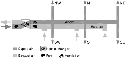
The building is equipped with a balanced mechanical ventilation system. A heat exchanger is placed between exhaust and supply air flows. Furthermore, a humidifier can be used to maintain the humidity level of supply air above 50% during the heating season.

This ventilation system introduces a certain degree of "thermal mixing" in the building, since all zones have the same supply air temperature. A simplified scheme is shown in Figure 6.

Supply air

Supply

Exhaust

Exhaust air

Heat exchanger

Fan Humidifier N

S

NW NE

SE SW

Figure 6: Ventilation

Each zone is assumed to be occupied by 2 persons. Office workers are supposed to enter the building at 8 AM and to leave the building at 6 PM during working day (from Monday to Friday). This fixed schedule is maintained during the whole year.

COMPARED CONTROLLERS

Reference controller

This controller is based on a feed-forward action on water supply temperature by the so-called "heating curve" and a feedback action on water flow rate by a thermostatic valve. It implements an optimal start algorithm. One controller is used for each heating loop and the boiler temperature setpoint is set to the maximum of the computed setpoints for both loops.

Optimal controller

The optimal controller is based on the algorithm described here above. Two controllers are used in parallel (one for each heating loop), using a one-zone simplified model. The reference zones (the only ones simulated in the internal model) are N for the North loop and S for the South loop. Other zones are only taken into account by identical boundary conditions in the controller's internal model.

The weather forecasting routine simply uses previous day data as forecast for the current day. A previous study has shown that this simple solution allows the optimal controller to operate properly while providing a lower bound for the controller's performance (Kummert, 2001).

The cost function uses the quadratic-linear approximation mentioned here above. In particular, the PPD is approximated on the basis of the operative temperature only (Fanger's formulation normally uses the air and the mean radiant temperature independently). The energy cost is computed using the net heating energy delivered to the reference zones only. Different settings were tested for the relative weight of discomfort and energy (α in (3)).

RESULTS

The following graphs will present the energy and discomfort costs for the entire heating season in the (Jd,Je) plane. In each Figure, the best controller is

closer to the lower left corner of the graph (smaller cost for both energy and discomfort).

The "trajectory" of different controllers is obtained by varying some settings of the controllers themselves or some parameters of the simulation:

• Reference controller: the best internal settings of the optimal start algorithm were obtained by trial and error. The controller "trajectory" was obtained by varying the setting of thermostatic valves in all zones simultaneously (from 19.75 to 22.0°C)

• Optimal controller: The relative weights of discomfort and energy costs are changed through varying the α parameter in the cost function (3). Thermostatic valves in reference rooms (S and N) are fully opened and other thermostatic valves are left to their nominal setpoint (21.0°C).

Performance in the reference zones

The results obtained in the two reference zones (N and S) are shown in Figure 7.

1000 1200 1400 1600 1800 2000 2200

0 500 1000 1500 2000 2500 3000

Jd [%PPD' h]

Je [

kW

h

]

Zone N, Reference Controller Zone N, Optimal Controller Zone S, Reference controller Zone S, Optimal controller

Figure 7: Performance in reference zones (N and S)

The North zone has far lower solar gains than the South zone. This explains the higher energy consumption and the lower discomfort: no overheating occurs and the installed heating power is sufficient to maintain the desired comfort temperature in all circumstances. A non-zero discomfort cost is only observed when heating is started too late in the morning (after night setback) or in case the setpoint is reduced below the "comfort range" in order to save energy.

The trajectories in the (Jd, Je) plane that are obtained

for both controllers are typical of all tested control algorithms (optimal and reference): for a well designed controller, it is only possible to reduce heating consumption by accepting a higher discomfort, which gives a roughly hyperbolic-like curve. The only exceptions are the ends of both curves for the South zone. For these extreme settings values, both controllers lead to a global decrease of performance (increased energy consumption and discomfort).

Performance in non-reference zones

Figure 8 shows the net energy cost and discomfort cost for the three Southern zones (S, SE, SW). Zones SE and SW are less subject to overheating and have a higher energy consumption than zone S because of lower solar gains. The difference between the SE and SW zones is explained by the higher fraction of useful solar gains in zone SE: direct solar radiation enters this zone during the morning, while most of solar gains in zone SW enter the zone at the very end of the occupancy period.

The behavior of non-reference zones is similar for both controllers. The optimal controller is still able to save energy in some conditions, but these energy savings are very limited (2 to 4%). Furthermore, the reference controller offers a larger range of discomfort cost. One should keep in mind that the simulation hypotheses are slightly different for both controllers: for the optimal controller, thermostatic valves in all rooms are set to 21°C in all cases, while the trajectory of the reference controller is obtained by varying the setting of all thermostatic valves simultaneously.

1000 1100 1200 1300 1400 1500

500 1000 1500 2000 2500

Jd [%PPD' h]

Je [

kW

h

]

Zone SW, Reference controller Zone SW, Optimal controller Zone SE, Reference controller Zone SE, Optimal controller Zone S, Reference controller Zone S, Optimal controller

Figure 8: Performance in all South zones

The situation in Northern zones is shown in Figure 9. Note that the scale of the Figures 8 and 9 is different: Northern zones have a higher energy cost (less solar gains) and a lower discomfort cost (no overheating). The optimal controller gives a very similar performance for all settings in NE and NW zones. Both the NE and NW zones have a higher energy cost than the reference zone (N) – note that this is not the case for the reference controller. Here again, all zones have a lower energy cost with the optimal controller.

The poor control of comfort level in non-reference rooms can be explained as follows: if a high comfort level is desired, the temperature in the reference zone is maintained at desired level in all circumstances. As radiators of the other zones are slightly oversized and equipped with thermostatic valves, these zones experience a good level of comfort. If the optimal controller attempts to save more energy by reducing the level of comfort, it slightly under-heats the

reference room, but this has almost no effect on other Northern rooms. If the optimal controller is used with a high weighting factor for energy, the water setpoint profile may become quite erratic with large oscillations sometimes caused by the PID algorithm. This gives a water setpoint adapted to zone N but not adapted at all for other zones. This can lead to a global decrease of the optimal controller performance for these zones (higher energy cost and discomfort cost).

1700 1800 1900 2000 2100

0 20 40 60 80 100

Jd [%PPD' h]

Je [

kW

h

]

Zone NW, Reference Controller Zone NW, Optimal Controller Zone NE, Reference Controller Zone NE, Optimal Controller Zone N, Reference Controller Zone N, Optimal Controller

Figure 9: Performance in all North zones

Global performance at the building level

Figure 10 shows the costs obtained for the group of Northern zones (N, NE and NW), the group of Southern zones (S, SE and SW) and for the whole building.

The total energy cost is simply obtained by summing the respective costs for all zones. The calculation of a total discomfort cost could use weighting factors to give more importance to given zones (e.g. with higher occupancy). In our case, we assumed an identical number of occupants in each zone. The discomfort cost is based on a Predicted Percentage of Dissatisfied, so the (possibly weighted) average between all zones is an expression of the cost (PPD) at the building level. Since we are only interested in the relative performance of two controllers, the sum of discomfort costs provides the same information and was used in Figure 10 to obtain a graphical presentation consistent with the energy cost.

3000 4000 5000 6000 7000 8000 9000 10000 11000

0 1000 2000 3000 4000 5000 6000 7000 8000

Jd [%PPD' h]

Je [

kW

h

] Whole building, Reference controller

Whole building, Optimal controller Northern zones, Reference controller Northern zones, Optimal controller Southern zones, Reference controller Southern zones, Optimal controller

The performance obtained for the entire building reflects the relative importance of different zones. The conclusions are therefore very dependent on the chosen example (6 zones of equal importance, of which 2 reference zones). It can be seen that the global performance of the whole building with both controllers is very similar to the behavior of a single-zone building (with a hyperbolic-like trajectory in the (Jd, Je) plane). The advantage of the optimal

controller is reduced to about 5% energy savings for a similar discomfort in the low discomfort range, and the reference controller performs better for high discomfort values (which are unlikely to be chosen by a building manager).

Detailed discomfort evaluation

Figure 11 shows the discomfort cost obtained for Southern zones with the optimal controller, according to simplified and detailed computations. As explained here above, the simplified cost is used by the optimal controller and the purpose of this comparison is to assess whether or not the optimization of a simplified discomfort cost also minimizes the actual discomfort of the occupants.

1000 1100 1200 1300 1400

400 1000 1600 2200 2800

Jd [%PPD' h]

Je [kW

h

]

Zone SW, Jd Zone SW, Jd (Detailed) Zone SE,Jd Zone SE, Jd (Detailed) Zone S, Jd Zone S, Jd (Detailed)

Figure 11: Detailed vs. simplified discomfort cost

Taking into account the actual humidity of the zones and both the air and mean surface temperatures causes a significant change in the computed discomfort (curves are shifted towards lower Jd

values). However, the relative position of the different curves remains similar.

A detailed study (not shown here) has shown that the most important factor that is neglected in the simplified discomfort cost is humidity. The consideration of the operative temperature instead of the mean radiant and air temperatures has no significant effect on the discomfort cost in our study. During the heating season, the relative humidity is often lower than 50%, despite the presence of a humidifier for ventilation air (the supply air humidity is controlled but not its temperature, which is lower than the average zone temperature).

This lower humidity actually reduces the computed discomfort during overheating periods, since the

human body is less sensitive to overheating in dry air, according to Fanger's comfort indexes. In the left part of each curve, discomfort is mostly caused by overheating and is less important when computed using the detailed definition.

For higher values of discomfort (right part of each curve), cold-related discomfort becomes more important. In this region, the effect of humidity is inverted, making computed cost higher when the detailed expression is used. The discomfort values obtained for Northern zones with the detailed cost function are therefore slightly higher than values obtained with the simplified expression.

The relative position of the different curves is not significantly modified for these thermal zones either. Globally, the relative performance of the optimal controller (i.e. compared to the reference controller) is slightly better with the detailed expression of discomfort cost than with the simplified expression.

Detailed energy cost (primary energy)

The primary energy consumption calculated by the detailed simulation model is used to assess the performance of both controllers. The purpose of this comparison is to assess whether or not optimizing the net energy delivered to the reference zones also minimizes the primary energy consumed at the building level.

Taking this into account, the primary energy does not modify the relative performance of different controllers in this simulation exercise. This is illustrated in Figure 12. This figure represents the net and primary energy consumption of the whole building versus the discomfort cost evaluated with the detailed expression. It can be compared with Figure 10 to evaluate the influence of the detailed discomfort cost expression on global performance results.

9000 9500 10000 10500 11000 11500 12000 12500 13000

2000 3000 4000 5000 6000 7000

Jd [%PPD' h]

Je [

k

W

h

]

J

e

,p

[

k

W

h

p

rim

ary en

e

rg

y

]

Je,p, Reference controller Je,p, Optimal controller Je, Reference controller Je, Optimal controller

Figure 12: Performance at the building level, detailed energy cost and detailed discomfort cost

are very similar for different controllers. The boiler efficiency is also very similar for all simulated cases. The global ratio between total net heat transferred to all zones and primary energy consumption is about 81% in all cases (ranging from 80% to 82%). Pipes heat losses represent about 6% of total heat load and the average boiler efficiency is about 86%, with the retained parameters for the simulation.

CONCLUSIONS

This simulation exercise aimed at assessing the performance of a single-zone optimal controller on a multizone building using a detailed simulation environment. The comparison with an advanced reference controller, including an optimal start algorithm, shows a slightly better global performance of the optimal controller. The latter leads to a better control of the reference rooms, despite strong simplifications in the controller's internal model, but it is not able to achieve a significantly better control of other rooms, especially if these rooms are not subject to overheating.

An improved algorithm taking the multizone character of the building into account would probably give better results, but further work is required to simplify the optimum search algorithm and to insure the robustness of such a controller. The relatively low financial incentives to implement advanced heating control strategies and the increased difficulty of commissioning controllers using complex algorithms are two obstacles to their implementation. Nevertheless, they can play a significant role in the global effort to reduce the energy intensity of buildings. The situation is different in cooling applications, where predictive controllers can take advantage of real-time electricity pricing and yield very substantial financial savings. Cooling and heating predictive controllers can share a great deal of hardware and software investments, which should then increase the financial gains of advanced heating control.

ACKNOWLEDGMENTS

This work has been partly funded by the European Commission, Directorate General XII (Contract JOE3-CT97-0076). The authors also wish to thank the Belgian national weather institute (Institut Royal Météorologique) for providing the real weather data used in the study.

REFERENCES

Braun J.E., 1990. Reducing energy cost and peak electrical demand through optimal control of building thermal storage. ASHRAE Transactions, Vol. 96, Nb. 2

Christoffers D. and Thron U. (Eds.), 2000. Development and test of modern control

techniques applied to solar buildings. Final Report, E.U. Research Contract JOE3-CT97-0076. European Union, Brussels, Belgium.

Fanger P.O., 1972. Thermal comfort analysis and application in environmental design. Mac Graw Hill.

Flake B.A., 1998. Parameter estimation and optimal supervisory control of chilled water plants. Ph. D. Thesis. University of Wisconsin-Madison

Henze G.P., Dodier R.H. and Krarti M., 1997. Development of a Predictive Optimal Controller for Thermal Energy Storage Systems. HVAC&R Research, Vol. 3, Nb. 3. pp 233-264.

Keeney K. and Braun J.E., 1996. A simplified method for determining optimal cooling control strategies for thermal storage in building mass. HVAC&R Research, Vol. 2, Nb. 1

Kummert M., 2001. Contribution to the application of modern control techniques to solar buildings. Simulation-based approach and experimental validation. Ph.D. Thesis. Fondation Universitaire Luxembourgeoise (Now University of Liège), Arlon, Belgium.

Kummert M., André Ph. and Nicolas J., 1996. Development of simplified models for solar buildings optimal control. in Proceedings of ISES Eurosun 96 congress. Freiburg

Kummert M., André Ph. and Nicolas J., 2001. Optimal heating control in a passive solar commercial building. Solar Energy, vol. 69 (0) pp. 103-116

Mozer, M.C., Vidmar, L., Dodier, R.H., 1997. The neurothermostat: predictive optimal control of residential heating systems. In Proceedings of Advances in Neural Information Processing Systems 9, MIT Press, Cambridge, MA, pp. 953-959.

Nygard-Fergusson A.-M., 1990. Predictive thermal control of building systems. Ph. D. Thesis. Ecole Polytechnique Fédérale de Lausanne

Oestreicher Y., Bauer M. and Scartezzini J.-L., 1996 Accounting free gains in a non residential building by means of an optimal stochastic controller. Energy and Buildings, Vol. 24, Nb. 3

The Mathworks, 1999. Using Matlab - Version 5.3, The MathWorks, Natick MA