The performance of Group Diffie-Hellman paradigms: a software framework and analysis

Rochester Institute of Technology

RIT Scholar Works

Theses

Thesis/Dissertation Collections

2007

The performance of Group Diffie-Hellman

paradigms: a software framework and analysis

Kieran S. Hagzan

Follow this and additional works at:

http://scholarworks.rit.edu/theses

Recommended Citation

The Performance of Group Diffie-Hellman

Paradigms:

A Software Framework and Analysis

March 4, 2007

Kieran S. Hagzan

[email protected]

Department of Computer Science

Rochester Institute of Technology

Thesis Committee:

Advisor: Dr. Hans-Peter Bischof

________________________________________

Reader: Dr. Edith Hemaspaandra

________________________________________

Observer: Prof. Phil White

________________________________________

S

UBMITTED TO THE

R

OCHESTER

I

NSTITUTE OF

T

ECHNOLOGY

IN PARTIAL FULFILLMENT OF THE REQUIREMENTS FOR THE DEGREE OF

M

ASTER OF

S

CIENCE

The Performance of Group Diffie-Hellman

Paradigms:

A Software Framework and Scalability Analysis

Abstract

un-The Performance of Group Diffie-Hellman

Paradigms:

A Software Framework and Scalability Analysis

Contents

1 Introduction

7

1.1 Problem Description

. . . .

7

1.2 Background

. . . .

8

1.2.1

Mathematical Notation

. . . .

8

1.2.2

Two-Party Diffie-Hellman Extended To Groups . . . 10

1.2.3

Linear Group Diffie-Hellman . . . 13

1.2.4

Tree-Based Group Diffie-Hellman

. . . 16

1.2.5

Hypercubic Group Diffie-Hellman

. . . 21

1.2.6

Hypothesis . . . 27

1.2.6.1

Linear Group Diffie-Hellman (LGDH) . . . 28

1.2.6.2

Tree-Based Group Diffie-Hellman (TGDH) . . . 30

1.2.6.3

Hypercubic Group Diffie-Hellman (HGDH) . . . 32

2 Methods

35

2.1 Software Design Model . . . 35

2.1.1

Internal I/O Handling

. . . 35

2.1.2

Topology Maintenance Abstraction . . . 37

2.1.3

Linear Group Diffie-Hellman Optimizations

. . . 38

2.1.4

Tree-Based Group Diffie-Hellman

. . . 38

2.1.5

Hypercubic Group Diffie-Hellman

. . . 39

2.2 Result Testbed . . . 40

2.2.1

Testbed Hardware Platform . . . 40

2.2.2

Result Collection . . . 40

2.2.3

Result Normalization . . . 40

3 Results

41

3.1 Raw Results . . . 41

3.1.1

LGDH . . . 41

3.1.2

TGDH . . . 42

3.1.3

HGDH . . . 43

3.1.4

Raw Combined Results . . . 44

3.2 Normalized Results . . . 45

3.2.1

LGDH . . . 45

3.2.2

TGDH . . . 46

3.2.3

HGDH . . . 47

4 Discussion

49

4.1 Variations Between Theory and Practice . . . 49

4.2 Causes of Variation . . . 49

4.3 Improvements / Future Work . . . 49

4.3.1

Key Sequencing . . . 49

4.3.2

Failure Detection . . . 50

4.3.3

Final End-User Interface . . . 50

5 Appendices

51

5.1 Result Data

. . . 51

5.1.1

LGDH . . . 51

5.1.2

TGDH . . . 53

5.1.3

HGDH . . . 55

5.2 Source Code . . . 57

5.2.1

v2/topo/tgdhTopology.java . . . 57

5.2.2

v2/topo/lgdhTopology.java . . . 65

5.2.3

v2/topo/hgdhTopology.java . . . 68

5.2.4

v2/topo/Node.java . . . 70

5.2.5

v2/topo/Topology.java . . . 71

5.2.6

v2/bin/Jumpstarter.java . . . 72

5.2.7

v2/utils/EnvironmentVariables.java

. . . 73

5.2.8

v2/utils/AddressConversion.java

. . . 75

5.2.9

v2/utils/BlockingFIFOQueue.java . . . 76

5.2.10 v2/utils/FIFOQueue.java . . . 77

5.2.11 v2/ka/KeyAgreement.java . . . 77

5.2.12 v2/ka/hgdhKeyAgreement.java . . . 78

5.2.13 v2/ka/lgdhKeyAgreement.java . . . 83

5.2.14 v2/ka/tgdhKeyAgreement.java

. . . 86

5.2.15 v2/ka/DiffieHellmanExchange.java . . . 91

5.2.16 v2/results/Collector.java . . . 92

5.2.17 v2/net/GroupSocket.java . . . 93

5.2.18 v2/net/Identifier.java . . . 99

5.2.19 v2/net/GroupManager.java . . . 108

5.2.20 v2/net/NetworkDevice.java . . . 118

5.2.21 v2/net/Reader.java . . . 123

5.2.22 v2/net/Decoder.java . . . 124

5.2.23 v2/net/State.java

. . . 128

5.2.24 v2/net/ProtocolConstants.java . . . 128

5.2.25 v2/net/Message.java . . . 129

5.2.32 v1/HGDH/Device.java

. . . 139

5.2.33 v1/HGDH/DiffieHellmanExchange.java . . . 141

5.2.34 v1/HGDH/Discoverer.java . . . 142

5.2.35 v1/HGDH/Jumpstarter.java . . . 142

5.2.36 v1/HGDH/Merger.java . . . 143

5.2.37 v1/HGDH/Message_OPC.java . . . 144

5.2.38 v1/HGDH/MessageProcessor.java . . . 144

5.2.39 v1/HGDH/Reactor.java . . . 158

5.2.40 v1/HGDH/Reader.java . . . 161

5.2.41 v1/HGDH/State.java . . . 162

5.2.42 v1/HGDH/MessageProcessor-OLD.java

. . . 163

5.2.43 v1/LGDH/Decoder.java . . . 176

5.2.44 v1/LGDH/Device.java . . . 179

5.2.45 v1/LGDH/DiffieHellmanExchange.java

. . . 180

5.2.46 v1/LGDH/Discoverer.java

. . . 182

5.2.47 v1/LGDH/Jumpstarter.java . . . 183

5.2.48 v1/LGDH/Merger.java

. . . 183

5.2.49 v1/LGDH/Message_OPC.java . . . 184

5.2.50 v1/LGDH/MessageProcessor.java . . . 185

5.2.51 v1/LGDH/Node.java . . . 196

5.2.52 v1/LGDH/Reactor.java . . . 198

5.2.53 v1/LGDH/Reader.java . . . 201

5.2.54 v1/LGDH/State.java

. . . 202

5.2.55 v1/LGDH/NodeArray.java . . . 203

5.2.56 v1/TGDH/Decoder.java . . . 206

5.2.57 v1/TGDH/Device.java . . . 209

5.2.58 v1/TGDH/DiffieHellmanExchange.java

. . . 211

5.2.59 v1/TGDH/Discoverer.java

. . . 213

5.2.60 v1/TGDH/Jumpstarter.java . . . 213

5.2.61 v1/TGDH/Merger.java

. . . 214

5.2.62 v1/TGDH/Message_OPC.java . . . 214

5.2.63 v1/TGDH/MessageProcessor.java . . . 215

5.2.64 v1/TGDH/Node.java . . . 228

5.2.65 v1/TGDH/Reactor.java . . . 229

5.2.66 v1/TGDH/Reader.java . . . 233

5.2.67 v1/TGDH/State.java

. . . 234

5.2.68 v1/TGDH/Tree.java . . . 234

1

Introduction

1.1

Problem Description

Today small, mobile computing devices such as PDA’s, laptops, tablet PC’s,

cellu-lar phones, etc. are being utilized as much as their cellu-larger stationary counterparts.

This has sparked the desire from end-users to experience the same functionality from

these mobile devices without compromised security. Mobile devices are typically

bat-tery powered and designed with energy-efficient hardware (memory, processor,

stor-age, peripherals, etc.) to conserve energy. Network media is typically wireless in

these environments, communicating within a given physical broadcast range. These

networks of devices are generally called “ad-hoc” networks due to their dynamic

na-ture. This is clearly a new environment where scalability is necessary to preserve

energy and compensate for the increased complexity of mobile network topology and

security algorithms. As protocols used for maintaining mobile ad-hoc networks are

mainly broadcast-based, the classical problems of point-to-point network computing

evolve from two-party problems into arbitrary-party problems.

Data security has three main facets: confidentiality, integrity, and authenticity,

typically accomplished through encryption, signatures, and hashing respectively. These

algorithms typically utilize security keys as input, forcing security key generation

al-gorithms to be addressed before the security alal-gorithms themselves can proceed. In

ad-hoc networks, a shared security key is required between all “trusted” devices in the

network to secure broadcast transmissions. In addition, each device in an ad-hoc

net-work is not required to be within the transmission range of every other device in the

network (fore more info, see Obraczka et al. [2001]). In this scenario, security keys

should change whenever the network topology changes, as well as on a regular basis

to force forward and backward security. This high quantity of key agreement

itera-tions combined with minimized computing resources further bolsters the requirement

for scalability of implementation.

1.2

Background

1.2.1

Mathematical Notation

Note: Information in this section is summarized from the contents of Trappe and Washington

[2002, pp63-103]

Groups, Rings, and Fields:

• Groups

–

A

binary operation

on a set

S

is an operation that maps a pair

(

a, b

)

∈

S

×

S

to a value

a

∈

S

.

–

A group

G

is a 2-tuple,

(

S,

∗

)

where

S

is a set and

∗

is a binary operation

upon that set. The group must fulfill three specific properties:

1. The group must be associative over the set

S

, i.e.,

a

∗

(

b

∗

c

) = (

a

∗

b

)

∗

c

for all

a, b, c

∈

S.

2. The group must define an identity element

i

such that

a

∗

i

=

i

∗

a

=

a

for all

a

∈

S

.

3. The group must define an inverse element

a

such that

a

∗

a

=

a

∗

a

=

1

for all

a

∈

S

–

If

a

∗

b

=

b

∗

a

for all

a, b

∈

S

, a group

G

is considered a commutative or

abelian group.

–

A group is considered finite if

|

G

|

is finite.

|

G

|

denotes the order of

G

.

–

A group

G

is denoted a

cyclic group

if there exists a

g

∈

G

such that for all

b

∈

G

there exists an integer value

i

where

b

=

g

. Such a value

g

is denoted

a

generator

of the group

G

.

–

Every finite group of a prime order is cyclic.

• Rings

–

A ring is a 3-tuple

(

S,

+

,

×

)

where:

1.

S

is a set.

2.

+

and

×

are binary operations denoted “addition” and “multiplication”

respectively.

3.

(

S,

+)

is a commutative group with additive identity 0

4. The operation

×

is associative over the set

S

.

5. There exists a multiplicative identity of 1 where

1

×

a

=

a

×

1 =

a

for all

a

∈

S

.

• Fields

–

A field is a commutative ring

R

where all elements

{

i

∈

R, i

6

= 0

}

are

invert-ible elements.

–

F

denotes a

f inite f ield of order q

, where

|F |

=

q

and

q

is finite.

–

The elements

{

r

∈ F

, r

6

= 0

}

form a group over multiplication denoted

F

,

the

multiplicative group of

F

.

–

A generator of the group

F

q

is known as a

primitive element

of

F

.

Exponentiation and the Logarithm

• Exponentiation in

R

–

Exponentiation defined over the real numbers “

R

” is a function mapping

elements of

R

×

R

to

R

, denoted:

a

=

b

, {

a, b, c

∈

R

}.

–

The

logarithm

function is defined over the real numbers as the inverse function of

exponentiation, denoted:

log

(

a

) =

c, {a, b, c

∈

R

},

read “c

is the logarithm root

b

of

a.”

• Exponentiation in

Z

–

Mathematical functions defined over the integers “

Z

” belong to a class of

functions known as

discrete f unctions

. Discrete functions often utilize the

“congruence modulo” relation (or the remainder of integer division) over

equality, a discrete function that maps elements of

Z

×

Z

to elements in

Z

.

–

Congruence modulo a prime

n

generates a finite field of order

(

n

−

1)

. The

generator

g

of such a field is denoted a

primitve root

modulo

n

.

–

Modular exponentiation is the discrete equivalent of exponentiation over

the real numbers, denoted:

a

≡

b

(

mod n

)

,

{

a, b, c, n

∈

Z

}

–

The discrete logarithm function is defined over the integers as the inverse

function of modular exponentiation, denoted:

L

(

a

)

≡

c

(

mod n

)

,

{

a, b, c, n

∈

Z

}

read “

c

is congruent to the

discrete logarithm

root

b

of

a

, modulo

n

”.

1.2.2

Two-Party Diffie-Hellman Extended To Groups

•

The Two-Party Diffie-Hellman Protocol

In 1976, W. Diffie and M.E. Hellman published “New Directions in

Cryptogra-phy,” introducing their two-party key-agreement protocol. The protocol was intended

to exchange a secret key over an insecure medium, and is based upon the difficulty of

computing the discrete logarithm in a finite field. The exchange protocol proceeds as

follows (from Trappe and Washington [2002, pp210-211] ):

Precondition:

Two Parties, “Alice” and “Bob”, share public values

p

(a large prime,) and

g

(a primitive

root modulo

p

.)

Alice

Bob

1.) Alice generates a random private value

x

, and computes the public value:

p

=

g

xa

(

mod p

)

1.) Bob generates a random private value

x

, and computes the public value:

p

=

g

xb

(

mod p

)

2.) Alice sends

p

and receives

p

.

2.) Bob sends

p

and receives

p

.

3.) Alice computes shared key

k

:

k

=

p

kB

(

mod p

)

=

(

g

xb

)

(

mod p

)

=

g

(

mod p

)

3.) Bob computes shared key

k

:

k

=

p

kA

(

mod p

)

=

(

g

xa

)

(

mod p

)

=

g

(

mod p

)

Table 1

•

The Security of Diffie-Hellman

In the Diffie-Hellman protocol, the shared key

k

is mathematically the result of

exponentiation modulo

p

. If the values

g, p, p

,

and

p

are public, an attacker would

need to determine the value of

x

x

by computing the discrete logarithm root

g

modulo

p

of both

p

and

p

. Knowing only the public values of the protocol, this is

considered mathematically infeasible, provided

p

is chosen as a “significantly large”

prime and

g

is truly a primitive root modulo

p

. Considering the relation of

congruence modulo

n

maps elements of the natural numbers to a finite field of order

(

p

−

1)

, many exponents of

g

can produce the public keys

p

and

p

, since

g

is a

generator of the cyclic group of order

(

p

−

1)

. If

p

is sufficiently large, then an

exhaustive search through all the

(

p

−

1)

possible exponents of

g

to determine the set

to a “man-in-the-middle” attack. In this attack, Eve intercepts

p

from Alice and

sends the public key

p

to Bob. Eve then intercepts

p

from Bob and sends

p

to

Alice. At this point, Alice and Eve have established key

k

and Eve and Bob key

k

.

Eve can now intercept messages from Alice, modify and inspect the message

contents, and transmit to Bob. Eve can also intercept messages from Bob and

transmit to Alice maliciously. This attack is possible since no authentication of Alice

or Bob is done during the protocol exchange. Solutions to this form of attack

classically include digital signatures and certificates based upon public/private

key-pairs obtained prior to a run of the Diffie-Hellman protocol. More recently,

modified protocols certify Diffie-Hellman based public-keys before two parties

exchange them.

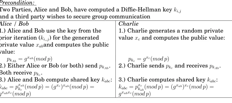
• Extending Diffie-Hellman

The generic two-party Diffie-Hellman algorithm can be extended to groups as

fol-lows (from Steiner et al. [1996]) :

Precondition:

Two Parties, Alice and Bob, have computed a Diffie-Hellman key

k

and a third party wishes to secure group communication

Alice / Bob

Charlie

1.) Alice and Bob use the key from the

prior iteration (

k

) for the generated

private value

x

and computes the public

value:

1.) Charlie generates a random private

value

x

and computes the public value:

p

=

g

xab

(

mod p

)

p

kc

=

g

xc

(

mod p

)

2.) Either Alice or Bob (or both) send

p

.

Both receive

p

.

2.) Charlie sends

p

and receives

p

.

3.) Alice and Bob compute shared key

k

:

3.) Charlie computes shared key

k

:

k

=

p

(

mod p

) = (

g

)

(

mod p

) =

g

(

mod p

)

k

=

p

(

mod p

) = (

g

)

(

mod p

) =

g

(

mod p

)

Table 2

In general, to extend the Diffie-Hellman algorithm to a third party using the

orig-inal two-party (Alice and Bob) algorithm (call the third party “Charlie”), Alice and

Bob first perform the typical Diffie-Hellman exchange. The key value from a prior

exchange denoted

k

is then used by the Alice and Bob as the private

contribu-tion to a second Diffie-Hellman exchange with Charlie. Charlie broadcasts his

pub-lic key

p

and thus both Alice and Bob are able to compute the second-round

Diffie-Hellman key as can charlie after receiving public key

p

. This process can be

In general, Diffie-Hellman key agreement is a function over

Z

p

that maps

{

[

x

, x

]

∈

Z

p

×

Z

}

to

{

k

∈

Z

}

if

p

and

g

are constant (Trappe and Washington [2002,

pp210-211]). To extend this notion to groups, the notion of a group itself must be clearly

defined. In cryptography and data networking, groups and networks are typically

synonymous in syntax and semantics, and in formal definition. In this work, a

net-work or group is formally defined as a collection of two or more nodes arranged in a

defined topology with a defined interconnection mechanism between the nodes. The

Diffie-Hellman algorithm may be custom-tailored iteratively or recursively to

tra-verse a given topology in a manner dependent upon the interconnection mechanism.

The following sections illustrate the linear, tree-based, and interconnection

mech-anisms for extending Diffie-Hellman to groups. These three connection mechmech-anisms

were chosen following research of the works Amir et al. [2001] and Amir et al. [2002]because

the communication and computational cost for each is predictable based on the data

structure of the implementation and as such the implementation should approximate

our theoretical predictions. In each algorithm definition, we assume an underlying

vector for the storage of nodes, with each node at a position

p

in the storage vector.

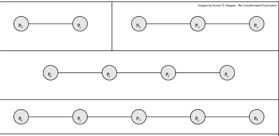
1.2.3

Linear Group Diffie-Hellman

•

Topology and Interconnection Mechanism

Consider a group of

n

nodes arranged in a vector or list at indices

0

through

n

−

1

,

with an interconnection mechanism as follows:

Figure 1

In the case of Linear Group Diffie-Hellman, we define the interconnection network

as two connections for each node at position

p

, the “left” connection to the node at

position

p

and the “right” connection to the node at

p

as shown in Figure 1. There

exists no connection on the left of node

p

nor to the right of node

p

.

• Topology Maintenance

1. Network Sponsorship

The node at the highest index

n

−

1

in the storage vector is designated

the network sponsor. The sponsor is responsible for maintaining any

alter-ations that occur to the topology.

2. Addition

Upon addition to the array, nodes are inserted at the

n

th position in

the storage vector, and network sponsorship and connectivity are updated

accordingly.

3. Removal

Upon removal from the array, a node in position

p

is deleted from

the storage vector, the positions of all nodes with index greater than

p

are

4. Merging/Partitioning

To merge two arrays

a

and

a

, the storage vector representing

a

is

concatenated to the vector representing

a

, then network sponsorship and

connectivity are updated accordingly. Partitioning a set of nodes

s

out of an

array

a

occurs by performing a removal operation of each element in the set

s

on the array

a

.

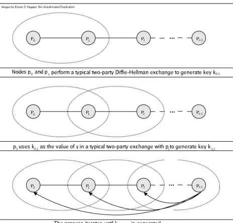
vector of nodes from lowest index to highest based on the methods in section(1.2.2).

The notion of Linear GDH was extruded from the CLIQUES protocol of Steiner et al.

[1998]. Shown in Figure 2, initially the nodes at position

p

and

p

perform a

two-party Diffie-Hellman exchange, using privately generated contributions of

x

and

x

to compute the public keys

p

and

p

, swapping them to computing key

k

. Node

p

then uses the computed value of

k

as the private contribution

x

in an exchange

with node

p

.

p

uses privately generated contribution

x

to compute public key

p

and

p

generates a new “combined” public key

p

from

x

(which again, is the computed

key

k

from the last round). The process is repeated up to node

p

, i.e. node

p

contributes

k

in a two party exchange with node

p

to generate combined public

key

p

(for all

i >

0

) and node

p

uses contribution

x

to generate public key

p

until

i

+ 1 =

n

−

1

. When a key exchange occurs between the nodes at indices

n

−

2

and

n

−

1

,

the node at index

n

−

1

is aware of the “plain” public keys

p

and

p

as well as “combined” public keys

p

for

0

< i < n

−

1

. The keys are then broadcast

to the remaining nodes

p

for

0

< i < n

−

1

, who must compute all keys

k

for all

i < n

−

2

(the rightmost node computes the group key in its first and only exchange).

Mathematically the group key

k

is computed as:

k

= (

g

)

(

mod p

) =

g

(

mod p

)

k

= (

g

)

(

mod p

) =

g

(

mod p

)

1.2.4

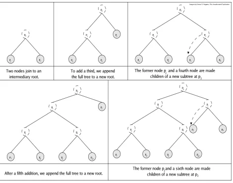
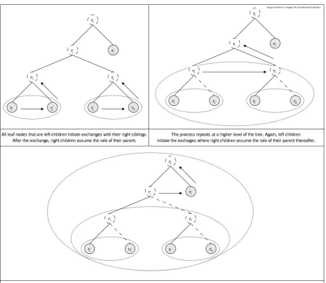
Tree-Based Group Diffie-Hellman

• Topology and Interconnection Mechanism

Consider a group of

n

nodes arranged in a list or array representing the leaves of

a binary tree, with an interconnection network as follows:

Figure 3

Tree-based Group Diffie-Hellman is implemented based upon the work of Kim et al.

[2002]. In the case of TGDH, an interconnection network is defined as three

connec-tions for each node at position

p

in the storage vector. The “parent” connection to

a node is at position [

(

p

−

1)

/

2

], the “left child” connection of a node is at position

• Topology Maintenance

The Tree-Based Group Diffie-Hellman protocol assumes that the binary

tree is maintained such that all true computing “devices” are at the leaves of

the binary tree. All non-leaf nodes are denoted

intermediary

nodes, intended

as “place-holders” during key agreement and key computation. In the above

diagrams, nodes with dashed borders are intermediary nodes, filled nodes with

solid borders are actual computing devices.

1. Network Sponsorship

The rightmost leaf-node in the topology is designated the network

spon-sor. The sponsor is responsible for maintaining any alterations that occur

to the topology.

2. Addition

Addition to the tree occurs in a manner dependent on the tree’s

com-pletion. If the tree is complete, then the existing tree is appended as the

left subtree of a new intermediary root node, and the joining node is added

as its right sibling. If the tree is complete, the leftmost-shallow node is

appended as the left child of a new subtree rooted at the leftmost-shallow

position, and the joining node is added as its sibling (see

Figure 3

.)

3. Removal

It is possible to decrease the depth of the tree and preserve left-to-right

filling upon removal from a tree, dependent on the type (intermediary or

actual) of the sibling of the node considered (

p

) for removal.

If the sibling of

p

is a leaf node:

If the sibling of the node to be deleted is a leaf node (node

p

in the top-right

illustration of Figure 3) then the sibling of

p

is stored in a temporary

lo-cation and the subtree rooted at

p

’s “uncle” (parent’s sibling) is “promoted”

to be

p

’s parent. The original sibling of

p

is then returned from temporary

storage via normal addition to the tree.

If the sibling of

p

is an intermediary node:

If the sibling of the node to be deleted is an intermediary node (node

p

in the

bottom-left illustration of Figure 3) then the subtree rooted at

p

’s sibling is

promoted to be its parent.

1. Merging/Partitioning

Merging two trees

t

and

t

occurs by “pruning” or collecting the leaf nodes

of

t

and performing a single addition for each to

t

. Partitioning a set of nodes

• Tree-Based Diffie-Hellman Propagation

Figure 4

In the case of Tree-Based Group Diffie-Hellman, extending the typical

two-party algorithm to groups requires applying the algorithm recursively in a

depth-first, upward propagation through the topology. The general algorithm proceeds by

computing keys for all non-leaf nodes in the topology, using the contributions

x

...x

(a) All leaf nodes check the current topology to determine first if the node is

the left or right child of its parent, and secondly if its sibling is a leaf or

intermediary node.

(b) If the node represents a left child:

i. It will initialize a two-party exchange with:

A. Either the sibling directly if the sibling is a leaf

B. Or the node “representing” the sibling (the rightmost leaf node of

the subtree rooted at the sibling) if the sibling is an intermediary.

and then listen for public key broadcasts. Otherwise,

(c) If the node represents a right child:

i. The node will wait until either:

A. Its sibling directly, or

B. The node representing its sibling

initializes an exchange with it. After a two-party key is computed and

public-keys are broadcast, this right sibling then assumes the role (becomes

“representative”) of its parent.

In this algorithm, key generation begins in the leaf nodes and proceeds toward the

root with Diffie-Hellman exchanges taking place between sibling nodes at the same

depth. After an exchange, if a node is a left child of its parent, it simply waits for

the broadcast of the public-key tree. Mathematically, a key between siblings

k

is

computed as follows for any right child

r

using private contribution

x

and sibling

l

who has public key

p

:

k

= (

g

)

(

mod p

) =

g

(

mod p

)

After the computation of

k

if the parent of the siblings is not the root, the right

sibling will then promote itself to be the parent, and use the value of

k

as a private

contribution to compute the “combined” public key

p

and the left sibling waits for a

broadcast of all public keys in the tree. If the parent is the root, the right node

broad-casts the tree of all public keys (plain at the leaves and combined for the internal

nodes), at which point all nodes can compute the keys for nodes between themselves

and the root, eventually computing the group key at the root. In the top center

il-lustration of Figure 3, the group key

k

at node

p

is computed from an exchange

between nodes

p

and

p

as follows:

1. The private contribution of node

p

(denoted

k

) is computed by a Diffie-Hellman

exchange between

p

and

p

:

For node

p

, the value of

k

= (

g

x3

)

(

mod p

) =

g

(

mod p

)

For node

p

, the value of

k

= (

g

x4

)

(

mod p

) =

g

(

mod p

)

2. The node

p

promotes itself to be the active node

p

, using

k

as private

3. An exchange is then performed between

p

and sibling node

p

.

p

uses public

key

p

from its privately generated contribution

x

as follows:

For node

p

, the value of

k

is

k

= (

g

x1

)

(

mod p

) =

g

(

mod p

) =

g

(

mod p

) =

g

(

mod p

)

which follows from step 1 and for node

p

the value of

k

is

k

= (

g

x2

)

(

mod p

) =

g

(

mod p

)

Following the progression of steps to see the computation of key

k

, we can see that

1.2.5

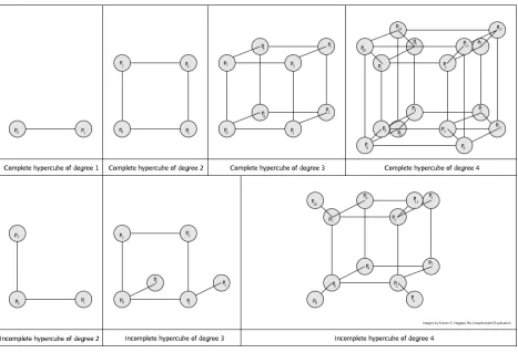
Hypercubic Group Diffie-Hellman

• Topology and Interconnection Mechanism

Consider a group of

n

nodes arranged in a list or array representing a hypercube,

with an interconnection network as follows:

Figure 5

Hypercubic Group Diffie-Hellman is based upon the “Octopus Protocol” described

by Becker and Wille [1998]. The notion of the octopus protocol is minimizing the total

number of Diffie-Hellman exchanges in the overall group. The other advantage of

the hypercube is that using our Gray Code mapping the structure fits into an array

perfectly with no wasted space as in the tree-based model, allowing for a minimum

data transfer when the group changes to re-key (McGrew and Sherman [1998]). In

the case of Hypercubic Group Diffie-Hellman, an interconnection network is defined

for each node based upon the degree, or dimension of the hypercube. The degree

of the hypercube is defined as the number of bits required to represent the highest

index(

n

−

1

) of the storage vector holding the nodes of the hypercube. For instance,

if the hypercube contains 8 nodes,

{

p

...p

}

, the hypercube is of degree 3, since 3 bits

are determined by “flipping” the the bits representing index

i

from most significant

bit to least. Flipping bits in this order guarantees that any tenticular nodes perform

their exchange with an inner node first to minimize synchronization issues later. For

example:

If the hypercube is of degree 4 containing up to 15 nodes, the node at

in-dex

p

would represent its index as 0000. Therefore, node

p

would have

connections to nodes with indices at {1000, 0100, 0010, 0001} in binary,

or

{

p

, p

, p

, p

}

.

Node

p

would represent its index as 0001 and have

connections with {1001, 0101, 0011, 0000} in binary, or

{

p

, p

, p

, p

}

. If

the degree of the hypercube were 5, node

p

would have connections with

{

p

, p

, p

, p

, p

}

and node

p

would have connections with

{

p

, p

, p

, p

, p

}

,

etc.

A hypercube is considered complete if the number of nodes contained is a even power

of 2. When a hypercube is complete, the interconnection network is as described

above. If the hypercube is incomplete (the number of nodes contained is not an exact

power of 2), those nodes with an index whose most significant bit is set to 1 are

con-sidered

tenticular

nodes. Tenticular nodes posses only a single connection to the node

whose index bitmask is that of the current node with the most significant bit flipped

to 0. In the diagram above,

p

, p

, p

, p

are tenticular nodes within the incomplete

hypercube of degree 4 and size 12. Note that

p

whose index is 1000 in binary has

only a connection to 0000, or

p

, 1001 to 0001, 1010 to 0010, and 1100 to 0100 in this

case. A hypercube node is

f ully connected

within its dimension if the node is either a

member of a complete hypercube, or is not a member of the outermost dimension of

an incomplete hypercube.

• Topology Maintenance

1. Network Sponsorship

The node at the last position

n

−

1

in the storage vector is designated

the network sponsor. The sponsor is responsible for maintaining any

alter-ations that occur to the topology.

2. Addition

Upon addition to the hypercube, nodes are inserted at a new

(

n

+ 1)

st

position in the storage vector, then network sponsorship and connectivity

are updated accordingly.

3. Removal

To merge two hypercubes

h

and

h

, the storage vector representing

h

is concatenated to the vector representing

h

, then network sponsorship

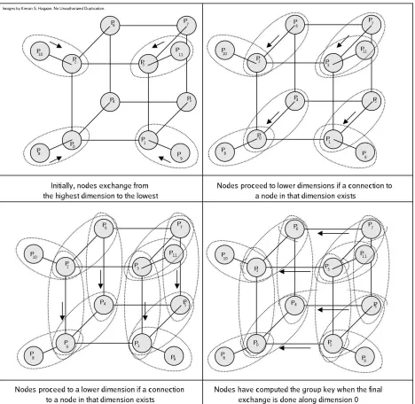
• Hypercubic Diffie-Hellman Propagation

Figure 6

In the case of Hypercubic Group Diffie-Hellman, extending the typical

two-party algorithm to groups requires for each node

p

, collapsing the hypercube based

1. Determine the index of node

p

ˆ

, the result of flipping the value of bit

k

in the

binary representation of the index

i

:

(a) If the node

p

ˆ

exists, perform an exchange with the node

(b) If the node

p

ˆ

does not exist, do nothing (this only happens when the outer

dimension of the hypercube is incomplete.)

2.

k

=

k

−

1

When

k

= 1

, then the sponsor node at array index 0 will broadcast the hypercube

of public keys to all nodes such that any tenticular nodes in an incomplete outer

dimension can generate the group key. In the bottom center illustration of Figure 3,

the nodes

p

and

p

would compute the group key as follows:

1. The highest dimension nodes of the hypercube (in this example

p

and

p

) will

exchange with their counterpart nodes found by flipping the most significant bit

of their index. In this example:

p

has index 4 with binary representation 100 which will exchange with index

000 or node

p

to compute key

k

k

= (

g

)

(

mod p

) =

g

(

mod p

)

p

has index 5 with binary representation 101 which will exchange with index

001 or node

p

to compute key

k

k

= (

g

)

(

mod p

) =

g

(

mod p

)

2. The outer dimension nodes

p

and

p

will now “freeze” and wait for the broadcast

of public keys subsequently by nodes

p

and

p

respectively. The inner

dimen-sion nodes will continue on to collapse on the dimendimen-sions of the structure, in this

example:

p

with binary representation 010 will exchange with node

p

with

represen-tation 000 to compute key

k

. In this exchange

p

will use the value of

k

computed in the outer dimension as its private contribution to compute public

key

p

.

k

= (

g

)

(

mod p

) = (

g

)

(

mod p

) =

g

x_4pk

0)pk₂

(

mod p

)

p

with binary representation 001 will exchange with node

p

with binary

rep-resentation 011 to compute

k

. In this exchange,

p

will use the value of

k

computed in the outer dimension as its private contribution to compute public

key

p

.

k

= (

g

)

(

mod p

) = (

g

)

(

mod p

) =

g

1)pk₃

(

mod p

)

3. A final exchange is computed along the innermost dimension:

p

with representation 001 will flip its least significant bit to exchange with

p

with binary representation 000 to compute the final key:

k

= (

g

)

(

mod p

) =

g

(

mod p

) =

g

(g(x4)(pk0))_pk 2)pk₁

p

with representation 011 will flip its least significant bit to exchange with

p

k

= (

g

)

(

mod p

) =

g

(

mod p

) =

g

(g(x5)(pk1))_pk 3)pk₂

4. Node

p

will send the public keys used in the exchanges with first

p

and secondly

p

to node

p

. At the time of the exchange with node

p

, node

p

used the value of

k

to generate public key

p

, so

p

can also generate

p

and compute first

k

as node

p

did in step 2 and then repeat step 3 exactly to produce key

k

. Node

p

will also send the public keys used in the exchanges with first

p

and secondly

p

to node

p

. At the time of the exchange with node

p

,

p

used the value of

k

to generate the public key

p

, so

p

can now also generate

p

and compute

1.2.6

Hypothesis

From Lee et al. [2002], heoretical bounds on the running times of each Group

Diffie-Hellman protocol are based upon the number of two-party Diffie-Diffie-Hellman

computa-tions performed by each node which in turn is based upon group size. Theoretical

bounds on network data transfer for each algorithm are based upon the count and

number of public-key broadcasts needed which is also based upon group size . This

section presents the predicted theoretical results of running time and data transfer

for the three paradigms. In each of the three cases, the data plotted is a

represen-tation of the complexity bound of the algorithm. When complexities are plotted, the

notion of an additive and multiplicative constant are allowed to compensate for

envi-ronmental factors. Therefore, the graphs that follow are meant to illustrate the rate

of change in experimental timing data expected as group size grows, not necessarily

meant to predict the experimental timing data for any given group size.

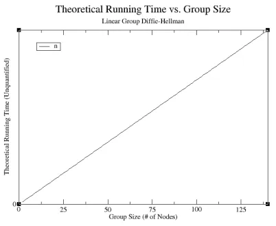
In general, when plotting a complexity of

n

for linear Group Diffie Hellman, this

actually implies the general plot of

cn

+

d

where

c

and

d

are constants, when

plot-ting

2(

n

−

1)

for tree based Group Diffie-Hellman, this implies the general formula of

1.2.6.1

Linear Group Diffie-Hellman (LGDH)

During an instance of the LGDH

protocol, each of the

n

nodes in the storage array could perform at most 2 exchanges,

one with their left partner, and one with their right. The node at position

p

has no left

partner and the node at

p

has no right partner, so the worst-case scenario occurs

for the node at position 0, who must perform

n

two-party computations.

Network data transfer consists of each node broadcasting at most 2 public keys,

the public key used in the exchange with their right partner, and the public key used

in the exchange with their left partner. The node at position

p

has no left partner and

the node at

p

has no right partner, so the total number of public keys broadcast to

determine the key for a group of size

n

is

2(

n

−

1) +

c

where

c

is a constant. LGDH

is an algorithm where at most two nodes at any given time are “active,” or currently

performing a two-party exchange.

1.2.6.2

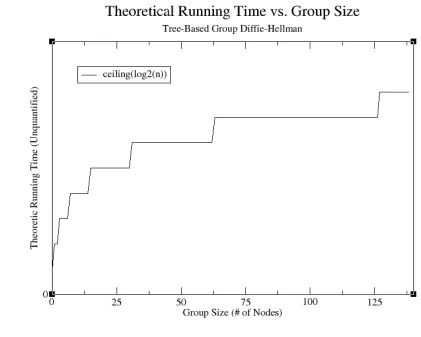
Tree-Based Group Diffie-Hellman (TGDH)

During an instance of the

TGDH protocol, the number of exchanges is proportional to the number of exchanges

per node multiplied by the node count. The number of exchanges per node is

propor-tional to the height of the tree at hand. The height of the tree at hand is proporpropor-tional

to the mathematical ceiling of the logarithm base 2 of the number of leaves in the

tree. For instance, a tree containing 7 nodes has a height of 3, therefore, each node

could perform at most three exchanges before computing the root key. Since there are

7 nodes, a total of 21 exchanges are performed in total. In general, for a tree of size

n

,

there are

ceiling

(

log

(

n

))

exchanges performed per node.

Network data transfer consists of two public-key broadcasts for all two-party

ex-changes. The number of two-party exchanges in total is equal to

n

∗

ceiling

(

log

(

n

))

,

and the number of key-broadcasts is therefore

2

n

∗

ceiling

(

log

(

n

))

. TGDH is an

1.2.6.3

Hypercubic Group Diffie-Hellman (HGDH)

During an instance of the

HGDH protocol, the number of exchanges is proportional to the number of exchanges

per node. The number of exchanges per node is proportional to the dimension of the

hypercube at hand. The dimension of the hypercube is proportional to the

mathe-matical ceiling of the logarithm base 2 of the number of nodes. For instance, a cube

containing 7 nodes is of dimension 3, therefore, each node could perform at most

three exchanges before computing the root key. Since there are 7 nodes, a total

of 21 exchanges are performed in total. In general, for a cube of size

n

, there are

ceiling

(

log

(

n

))

exchanges performed per node.

Network data transfer consists of two public-key broadcasts for each two-party

ex-change performed. Therefore, the number of public keys broadcast is

n

∗

ceiling

(

log

(

n

))

.

4. Discussion of Hypothesis

2

Methods

2.1

Software Design Model

2.1.1

Internal I/O Handling

To properly simulate a broadcast ad-hoc network environment within a wired

net-work, network packets are addressed to the network’s broadcast address. Typically,

the broadcast address for a network is the network portion of the network IP address

group masked with the network’s

subnet mask

(combine the IP and subnet mask with

the logical AND operation). Sending packets to this address allows for each node to

send exactly one packet which is theoretically received by all other hosts listening to

the broadcast address. Due to our broadcast addressing schema, UDP transport is

used over TCP transport, introducing packet-loss and forcing the robustness of the

underlying design. Efforts have been made by Adamson et al. [2000]to create reliable

multicast in this same fashion.

Introduced in the Java programming language version 1.4 was the notion of the

standard “select()” system call to perform I/O multiplexing, along with non-blocking

I/O. Typically, this technique is used to reduce CPU overhead by polling the native

network hardware to determine if there is any I/O to perform. If so, data is read to be

processed, a response is generated and sent, finally the CPU will return back to the

“select()” system call. If no I/O is ready, the CPU will either sit idle, or do some other

work that is lying around. This is accomplished by a multithreaded, event-driven

“reactor” pattern often used with large-scale and high-demand network programs.

One main thread will hand each event-request off to a child thread, who will then

do some work and die-off. Since the tasks performed by the child-threads are often

long-lived, the benefits of multithreading outweigh the overhead of thread-creation

and startup and is beneficial overall.

2.1.2

Topology Maintenance Abstraction

In order to standardize the topology management handler of the system, the

op-erations on the topology were generalized into four distinct opop-erations: join, leave,

merge, and partition. The bulk operations of merge and partition are often expressed

as multiple applications of join and leave. Depending on the topology however, the

bulk operations can occasionally be accomplished by a single operation. Regardless of

implementation, all Diffie-Hellman based key agreement strategies should be able to

support these three operations, under the following preconditions and postconditions:

Join:

Precondition:

One or more nodes exist in a group to join.

Postcondition:

The joining node is added to the topology representative of the key

agreement strategy at hand. The topology is distributed to all members, and the

key-agreement layer is notified to update the key collaboratively, ensuring forward

security.

Leave:

Precondition:

One or more nodes desires to leave an existing group.

Postcondition:

The leaving node is removed from the topology representative of the

key agreement strategy at hand. The topology is distributed to all members, and the

key-agreement layer is notified to update the key collaboratively, ensuring

backward-security.

Merge:

Precondition:

Two or more groups of nodes exist that wish to merge.

Postcondition:

The merging groups are combined into one larger group. The merged

topology is distributed to all members of both groups, and the key-agreement layer is

notified to update the key collaboratively, ensuring forward-security.

Partition:

Precondition:

A group of nodes wishes to leave the group at once.

Postcondition:

The leaving group is removed from the topology representative of

the key agreement strategy at hand. The topology is distributed to all members,

and the key-agreement layer is notified to update the key collaboratively, ensuring

backward-security.

2.1.3

Linear Group Diffie-Hellman Optimizations

Each exchange in the two-party GDH algorithm requires two broadcast messages,

one sent by a distinct party denoted

A

and received by another distinct party denoted

B

, and a second message sent by party

B

and received by party

A

, In the LGDH

proto-col, the manner in which this bi-directional communication occurs is not specified. In

this implementation key propagation occurs from left-to-right exclusively beginning

with nodes

p

and

p

and repeating until nodes

p

and nodes

p

compute the final

key. When the key reaches node

p

then all public keys used in the key computation

have been collected and the node at position

n

−

1

sends a broadcast message with the

public keys.

At this point the subkey

k

for all nodes

k

is computed with the public keys

from the broadcast message and this process is repeated for

k

all the way to

k

. Forcing a directional key propagation eliminates half of the synchronous

communication (backward propagation) that occurs within the LGDH protocol,

im-proving performance within small groups dramatically. Also, the structure is a

com-plete structure with no wasted space (every array element represents one actual

de-vice in the topology) and is therefore space-efficient. Finally, the protocol is a fully

event-driven protocol, meaning is is a “push” protocol and no node needs to poll any

other to determine if that node is ready to perform an exchange. When a leftmost

node initiates an exchange with its right neighbor, that neighbor is guaranteed to

be awaiting the request and should act immediately if that node is still alive. This

means synchronization latency from parallelism is 0.

2.1.4

Tree-Based Group Diffie-Hellman

To represent the binary tree as an array, the simple rule is that the children of

parent

i

are at index

2

i

+ 1

and

2(

i

+ 1)

for the left and right child respectively. A

depth-first search technique is used to find and traverse nodes in the tree, since

leaf-nodes are guaranteed to be mostly at the end of the tree’s storage array. Backward

propagation is again reduced by each right-child collecting the “blind-key” subtree of

their left sibling, and sending it to their parent’s right sibling if the parent is not the

root. If the parent is the root, the rightmost child broadcasts the “blind-key” tree, and

all nodes compute the shared key using the blind-keys on the path from themselves

to the root. Since the structure is partially-parallelized , there exists a substantial

amount of opportunity for synchronization latency, since right nodes that promote to

their parents must poll their right sibling to ensure the tree is synchronized.

Other-wise, the right sibling may not have computed the key from its leaves to its current

index, and both the left and right subtrees would determine different shared keys.

The protocol is also not space-efficient, since there could be as many as

2

nodes in

2.1.5

Hypercubic Group Diffie-Hellman

The hypercubic structure is a method often used to manage work-sharing and

distribution among a set of processors. Since the formation of a contributory key is

not much more than this, it is reasonable to apply the hypercubic notion to solve the

Diffie-Hellman shared-key problem. If the nodes of a hypercube are arranged using

a Gray Code mapping, then the cube maps perfectly onto an array structure. A Gray

Code is a binary position mapping where no two successive elements differ in only

one digit. Translated to our hypercube, in our notation two adjacent nodes in the

hypercube differ in only one dimension (one bit of their underlying positional index in

the storage vector). Furthermore, each node flipping the bits of their index from MSB

to LSB maps the traversal of the structure in linear time.

2.2

Result Testbed

2.2.1

Testbed Hardware Platform

The computing platform used for the testbed included 137 Sun SPARC-II machines

running between 440 and 650 MHz, containing between 256 and 512 MB. of memory.

The nodes are interconnected via a 100Mbps, fully-switched Ethernet which spans

one subnet. The testbed is a public-domain computing platform, so results were taken

over a 1 week period to get an average-load sample. The devices were assumed to

be fault-tolerant, thus no checks are performed to ensure that the device has not

experienced an error or has left the topology maliciously. Such data sets (when they

did occur) were discarded. Each node shared a common-filesystem via NFS, therefore

each node used a specific output file mutually-exclusive of all other nodes and stored

on each machine’s local filesystem to avoid synchronization and file-locking issues.

When the test-runs are complete, the output files are placed into the NFS directory

tree.

2.2.2

Result Collection

The results collected are in the form of transcripts for each node during each test

run. The transcripts are a log of the changes in group size, and the time needed to

compute the group key after the change. Each node went through different stages

of joining and merging until all available nodes were joined a group and computed

the group key, making each transcript a distinct data set. The transcripts were then

merged into one final result set by averaging the group size and time pairs to

deter-mine average cost per node. The testbed was then repeated 100 times over the course

of 1 week, and the final result sets of each test-run were averaged. This

double-averaging technique was done to eliminate erroneous data points automatically by

increasing the degree-of-freedom present for all data sets.

2.2.3

Result Normalization

3

Results

3.1

Raw Results

3.1.1

LGDH

3.1.2

TGDH

3.1.3

HGDH

3.1.4

Raw Combined Results

3.2

Normalized Results

3.2.1

LGDH

3.2.2

TGDH

3.2.3

HGDH

3.2.4

Normalized Combined Results

4

Discussion

4.1

Variations Between Theory and Practice

When the theoretical performance of software is considered, there are many

physi-cal and environmental circumstances that are ignored in theory but in practice cause

the performance of the solution to be less than optimal. In this particular case, the

largest hindrance that can be considered a static quantity for each node that

partici-pated in the tests is the NFS overhead. As mentioned earlier, the use of machine-local

files was incorporated to prevent this latency and the files were moved to NFS after

the timing-studies were taken.

When the results are analyzed, it is apparent that LGDH performed remarkably

better than expected, and HGDH performed remarkable worse than expected. The

theoretical bounds on HGDH are computationally the best, however of the parallel

al-gorithms, it performed worst. LGDH has a very poor theoretic computational bound,

but performs far better than its parallel counterparts up to 75 nodes. Since each

algorithm is optimized for its topology and traversal, a common I/O framework was

utilized for these purposes, and the results normalized over many iterations taken

during a 1 week span, these results can be considered a fair sample.

4.2

Causes of Variation

The real difference between the paradigms that causes the most latency is surely

the synchronization overhead of parallelism. The non-parallel paradigm (LGDH)

out-performed the parallel paradigms regardless of their ability to eliminate backward

propagation up to a reasonable size closed-network. Of the parallel paradigms, the

one that was “less parallel” (TGDH) outperformed the fully parallelized algorithm

(HGDH), even though TGDH uses a far larger memory footprint and computation per

node. Since there were no other measurable quantities of HGDH that could cause it to

perform more poorly than TGDH, the conclusion left is parallel latency. This latency

can also be used to explain the high-value at which the parallel algorithm benefits the

situation, since at that point the computational complexity of LGDH has rendered it

unusable in practice.

As mentioned, the memory footprint of TGDH and the “intermediary” nodes it

utilizes may become prohibitive for huge ad-hoc networks, at which time HGDH is

a feasible option. Regardless, LGDH is meant for ad-hoc networks of 100 devices or

less, at which point a new solution is needed.

4.3

Improvements / Future Work

4.3.1

Key Sequencing

number to each key, and therefore each encrypted message, telling the nodes which

key was used to encrypt each message. Security is not harmed since the sequence

numbers and keys are completely unrelated, and having the sequence number would

do nothing for an attacker. The second (and naive) solution would be to try all old

prior keys and perform syntactic and semantic-analysis on the result, choosing the

best match.

4.3.2

Failure Detection

As mentioned, this protocol (in its current state) does no form of failure detection.

That is, if a node were to leave unexpectedly or maliciously, the protocol could break.

It is designed to deal with lost packets, but identified nodes are expected to remain

healthy for the duration of the tests. The solution here is some form of heartbeat

mechanism that occurs in the same manner the protocol is traversed. When a node

finds an exchange-partner non-existent, broadcast this fact to all other nodes, each

check for their respective partner, and notify the “sponsor” accordingly, choosing a

new sponsor if necessary. At least this way, the solution to the heartbeat scheme

is guaranteed to follow the general complexity bound of the topology traversal and

key-agreement paradigm.

4.3.3

Final End-User Interface

5

Appendices

5.1

Result Data

5.1.1

LGDH

Group Size Key Agreement Time (Seconds)

2 0.40723045522018764 3 0.34250968456004405 4 0.3092227592267134 5 0.3263413407821234 6 0.3270269905533071 7 0.32522067957617856 8 0.3608326480263161 9 0.3613916773916764 10 0.39727102803738246 11 0.37408369408369435 12 0.3708730842911878 13 0.4356628029504741 14 0.48649070847851394 15 0.4547672514619889 16 0.45891850490196107 17 0.48103305322128764 18 0.5820204342273307 19 0.48977214377406914 20 0.5345782608695653 21 0.580240327380954 22 0.6025606060606067 23 0.5706601449275366 24 0.5660621468926555 25 0.7177409523809528 26 0.6885369230769207 27 0.6354879629629642 28 0.5807598214285723 29 0.6197308429118765 30 0.6376942857142865 31 0.6497195340501792 32 0.6472229729729739 33 0.6894715909090905 34 0.6490316742081447 35 0.7446600985221671 36 0.6031785714285723

Group Size Key Agreement Time (Seconds)

LGDH (Continued)

Group Size Key Agreement Time (Seconds)

73 1.0698862418106039 74 1.064197212837838 75 1.1822757575757565 76 1.1501273684210518 77 1.1236996047430823 78 1.1441995192307675 79 1.2176772151898716 80 1.1569484374999985 81 1.29274797786292 82 1.43955081300813 83 1.1959508032128516 84 1.2128286564625848 85 1.28389 86 1.2455799999999981 87 1.3406449553001278 88 1.42193899521531 89 1.393021535580528 90 1.30839312169312 91 1.3566505494505507 92 1.3976064311594214 93 1.5525178494623681 94 1.44853244680851 95 1.6711382775119628 96 1.6446921874999962 97 1.6861196772747646 98 1.4961938775510175 99 1.8552816627816644 100 1.773338846153844 101 1.9004873009040033 102 1.719240896358539 103 1.7228957928802566 104 1.7000725524475537 105 1.9086184873949599 106 1.7579456159822406 107 1.6360116822429922 108 2.053222993827158

Group Size Key Agreement Time (Seconds)

5.1.2

TGDH

Group Size Key Agreement Time (Seconds)

2 0.3393288174221315 3 0.19456511669339024 4 0.3090830970556164 5 0.302947270800212 6 0.3498852931752653 7 0.4118754221388373 8 0.5533706268221569 9 0.5361854808057775 10 0.47172351121423123 11 0.5630044733631558 12 0.5671471449487568 13 0.5662866015971627 14 0.6160350591112931 15 0.7178017241379314 16 0.7989032674118639 17 0.728303380782918 18 0.6728504716981102 19 0.7160832102412589 20 0.752962525667352 21 0.7021309699655357 22 0.7253411016949167 23 0.8786529411764705 24 0.866923406279732 25 0.8002461701003681 26 0.8531194029850748 27 0.8002145270270278 28 0.9585946097697923 29 1.128984757505773 30 0.940890318970341 31 1.0007456852791863 32 1.1614331328088852 33 1.1054333151878075 34 1.0746897983392636 36 1.0784567307692308 37 0.9263843098311826

Group Size Key Agreement Time (Seconds)

TGDH (Continued)

Group Size Key Agreement Time (Seconds)

76 1.2600213523131696

77 1.169613390928725

78 1.4338664122137454

79 1.334944055944058

80 1.2618336283185825

81 1.370316923076922

82 1.199572580645162

83 1.3108476027397262

84 1.2085167652859958

85 1.3874309133489442

86 1.402337962962966

87 1.3722058449809402

88 1.5232015065913398

89 1.1749632587859462

90 1.2161789667896663

91 1.1510899122807035

92 1.4709999999999994

93 0.9986541554959771

94 1.5524366197183086

95 1.2244631578947356

96 1.3688385416666697

97 1.514179028132992

98 2.5830134228187887

100 1.3815776397515613

101 1.5033061056105563

102 1.66192105263158

103 1.1885

104 1.1836555023923439

105 1.3628384798099769

106 1.3812065727699527

107 1.2581100917431194

108 1.5246451612903216

109 1.4608628048780483

111 1.285567567567568

112 1.243026785714284

Group Size Key Agreement Time (Seconds)

113 1.4570110619469017

114 1.4702882096069874

115 1.251

116 1.222339055793991

117 1.7483697478991598

118 1.7242711864406781

119 1.5069201680672248

120 1.238208333333333

121 1.1644508196721313

122 1.2867950819672136

123 1.7603008130081297

124 1.2439435483870958

125 1.4038293333333332

126 1.5440312500000006

127 1.7226850393700783

128 1.7461322957198493

129 1.5690775193798443

130 1.3234086294416234

132 1.3592989949748735

134 1.7298272058823532

5.1.3

HGDH

Group Size Key Agreement Time (Seconds)

2 0.28241318537859045 3 0.16426388115134605 4 0.3605236042692944 5 0.20211922639362961 6 0.46999611801242214 7 0.5158127373648852 8 0.6250615717821795 9 0.5191505167958665 10 0.5472925795052997 11 0.577521846370684 12 0.7729729080932788 13 0.6830138461538469 14 0.7628346833578799 15 0.8613180467091324 16 0.953971337579619 17 0.8301150708458563 18 0.8560633169934652 19 0.84255427631579 20 0.8476279999999989 21 0.8013449163449142 22 0.8207713358070522 23 0.8866375183194912 24 1.0612067307692297 25 0.9197626666666674 26 0.9166907484407476 27 0.926797078768912 28 1.097555194805193 29 1.0507347480106097 30 1.1847744791666666 31 1.21003444505194 32 1.2674879032258093 33 1.1785078201368517 34 1.1834582967515335 35 1.1762461904761912

Group Size Key Agreement Time (Seconds)

HGDH (Continued)

Group Size Key Agreement Time (Seconds)

70 1.5019010989010995 71 1.5193556338028154 72 1.7482881944444417 73 1.6742054794520524 74 1.7305094594594579 75 1.554417777777778 76 1.4805358851674626 77 1.55898311688