A comparison of satellite remote sensing data fusion methods to map peat swamp forest loss in Sumatra, Indonesia

A comparison of satellite remote sensing data fusion

methods to map peat swamp forest loss in Sumatra,

Indonesia

Merry Crowson1, Eleanor Warren-Thomas2, Jane K. Hill2, Bambang Hariyadi3, Fahmuddin Agus4, Asmadi Saad5, Keith C. Hamer6, Jenny A. Hodgson7, Winda D. Kartika3, Jennifer Lucey2,

Colin McClean8, Neneng Laela Nurida4, Etty Pratiwi4, Lindsay C. Stringer9, Caroline Ward9& Nathalie Pettorelli1

1_{Institute of Zoology, Zoological Society of London, Regent’s Park, London NW1 4RY, United Kingdom} 2_{Department of Biology, University of York, York YO10 5DD, United Kingdom}

3_{Biology Education Program, Faculty of Education and Teacher Training, Jambi University, Jl. Raya Jambi-Ma.Bulian km 15 Mendalo Darat, Jambi,}

Indonesia

4_{Indonesian Soil Research Institute, Indonesian Center for Agricultural Land Resources Research and Development, Jl. Tentara Pelajar No. 12,}

Cimanggu, Bogor 16114, Indonesia

5_{Soil Science Division, Faculty of Agriculture, Jambi University, Jl. Raya Jambi-Ma.Bulian km 15 Mendalo Darat, Jambi, Indonesia} 6_{School of Biology, Faculty of Biological Sciences, University of Leeds, Leeds LS2 9JT, United Kingdom}

7

Institute of Integrative Biology, University of Liverpool, Liverpool L69 7ZB, United Kingdom

8

Environment Department, University of York, Heslington, York YO10 5DD, United Kingdom

9

School of Earth and Environment, University of Leeds, Leeds LS2 9JT, United Kingdom

Keywords

Deforestation, land cover, peat swamp forest, restoration, satellite data fusion, tropical peatland

Correspondence

Nathalie Pettorelli, Institute of Zoology, Zoological Society of London, Regent’s Park, London NW1 4RY, United Kingdom. Tel: +44 020 7449 6334;

E-mail: [email protected]

Funding Information

This research was funded through the Newton Fund project “Enhancing the benefits of tropical peatland restoration for supporting local communities and ecosystem processes”, NERC Reference: NE/P014658/1.

Editor: Ned Horning Associate Editor: Moses Cho

Received: 4 July 2018; Revised: 8 November 2018; Accepted: 14 November 2018

doi: 10.1002/rse2.102

Remote Sensing in Ecology and Conservation2019;5(3):247–258

Abstract

Introduction

There is growing recognition of the importance of tropi-cal peatlands as globally significant carbon sinks and bio-diversity hotspots (Jaenicke et al. 2008; Dargie et al. 2017). The greatest extent of tropical peatland is in Southeast Asia (247 778 km2), of which 206 950 km2 is found in Indonesia (Page et al. 2011). The natural land cover in these peatlands is peat swamp forest, but logging, drainage, conversion to industrial plantations and fires have led to large-scale forest loss and degradation (Dohong et al. 2017). Peat swamp forests have been lost at a very fast rate: an estimated 73 000 km2of peat forest was lost across Sumatra, Kalimantan and Peninsular Malaysia between 1990 and 2015 (Miettinen et al. 2016). This has had devastating consequences for wildlife, partic-ularly peat swamp forest specialist species such as fresh-water fish and trees (Posa et al. 2011).

Peat consists of incompletely decomposed plant mate-rial that has accumulated over thousands of years in waterlogged environments that lack oxygen. The process of converting peat swamp forest to plantations involves draining the peat, in order to lower the water table and increase productivity. Not only does this land-use change reduce biodiversity, but dry peat oxidizes more quickly, releasing CO2into the atmosphere; dry peat is also more prone to fires (Page and Hooijer 2016). Fires affect drained peatland regularly in Indonesia, and during the very severe El Ni~no events in 1997 and 2015 very large areas of peat burned, causing hazardous levels of air pol-lution, posing a risk to human health (Chisholm et al. 2016) and causing economic losses estimated at 16.1 bil-lion USD in 2015 (World Bank, 2016). The economic impacts combined with fragmentation of habitat, release of a major carbon sink and threat of fire and smoke, has made peatland restoration a priority in the region (Gra-ham et al. 2017). Restoration aims to reinstate the envi-ronmental and economic services that tropical peatlands provide (Page et al. 2009). In Indonesia there is currently a focus on canal blocking in cultivated areas to re-wet drained peatland (Ritzema et al. 2014) and selecting appropriate restoration sites to replant with natural vege-tation (Graham et al. 2017).

In order to protect remnant peat swamp forest and locate optimum sites for peatland restoration efforts, it is essential to have up-to-date information on the extent and condition of peat swamp forests. The use of open source software and satellite remote sensing data allows cost-effective and standardized mapping of ecosystem extent and dynamics for large areas, at a high temporal resolution (Murray et al. 2018). Two main types of satel-lite remote sensing data can be used in forest mapping: optical and radar. These two types of sensors offer

complementary information about the Earth’s surface, as they operate based on different fundamental physical principles. Optical sensors passively measure electromag-netic radiation reflected from the Earth’s surface, enabling land cover mapping based on spectral reflectance; they are thus sensitive to cloud coverage. Radar sensors actively emit electromagnetic radiation in wavelengths that penetrate cloud, and measure the returning signal, so they are not affected by cloud cover. Radar responds to the three-dimensional structure of objects, so the signal returned for vegetation depends on the size, density, ori-entation and dielectric properties of elements comparable to the size of the radar wavelength, such as canopy or stems (Moreira et al. 2013).

Data fusion techniques are emerging as a powerful way to integrate information from the two complementary sensor types (Joshi et al. 2016). Peat swamp forests are generally found in areas with high cloud cover, which means that their distribution can potentially be mapped more reliably through the use of data fusion (Schulte to B€uhne and Pettorelli 2018). However, there are many dif-ferent data fusion techniques, and little information exists on how they compare (Schulte to Buhne and Pettorelli€ 2018). To fill this gap in knowledge, this study compares three common data fusion methods, applied to the map-ping of the remnant distribution of peat swamp forests in the area surrounding Sungai Buluh Protection Forest, Sumatra, Indonesia. The first data fusion method is a pixel-based classification using the original pixel values (OPVs), the second method uses an object-based classifi-cation, and the third method is a pixel-based classification using principal components (PCs).

Materials and Methods

Study area

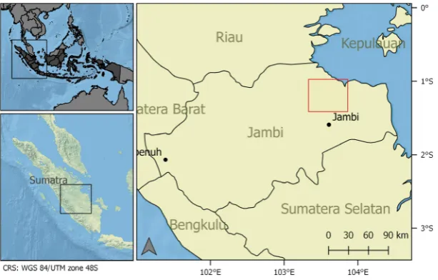
The study area covers 2874 km2 and is located in Jambi Province, Sumatra, Indonesia (Fig. 1). The area is located 40 km north of Jambi City, and predominantly falls within the East Tanjung Jabung Regency. Peatland covers a large part of the study area (Wetlands International 2003), but the original peat swamp forest cover has mostly been removed and replaced by plantations or lost in forest fires (Miettinen et al. 2016).

forest with a history of fires and disturbances (Hapsari et al. 2017). The forest is about 120 km2 in size, repre-senting about 4% of the study area. The study region also has areas of regrowth left unmanaged after severe fires, which are covered with ferns, shrub and other regrowth (Miettinen and Liew 2010). These fern-dominated areas cover approximately 3% of the study region and are thought to occur in areas where intense or frequent fires have severely degraded peatland, preventing a natural suc-cession back to tropical peat swamp forest (Page et al. 2009). The rest of the study region (approximately 8%) includes canals, rivers, roads and urban areas.

The climate in the region is tropical humid, with a mean annual temperature of 26°C and an annual rainfall of 2400 mm (Karger et al. 2016). The temperature varies little throughout the year but there is a slightly drier sea-son from June to September, corresponding to the onset of the southeast monsoon (Hapsari et al. 2017). However, even during this drier season average monthly precipita-tion remains above 100 mm, meaning that it is unlikely any seasonality will be seen in the vegetation due to water stress in the drier months.

The area is low-lying, with most of the study area less than 30 m asl. The highest point is 143 m asl and is found in the south-west of the study area. This means that the radar data will not show the foreshortening and layover effects that can be found in areas with steep relief (Moreira et al. 2013).

Remote sensing data

This study uses a C-band Sentinel-1 radar product and optical Sentinel-2 products from 2017 (Table 1). We

downloaded C-band dual polarized (VV+VH) Sentinel-1 Ground Range Detected Geo-referenced (GRD) products with a spatial resolution of 10 m, captured in Interfero-metric IW-mode. The Sentinel-2 data were available as Level 1C products and we used bands 2 to 8A, 11 and 12 throughout this study. All of the Sentinel-1 images are from relative orbit number 18 and the Sentinel-2 from relative orbit number 118.

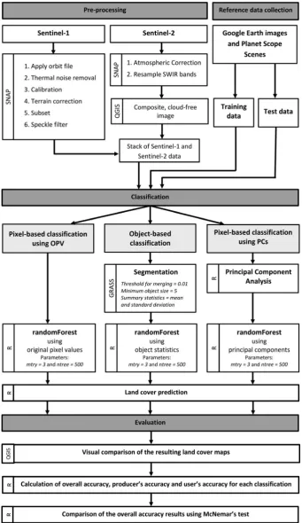
An overview of our pre-processing step and an outline of our workflow can be found in Figure 2. We pre-processed the Sentinel-1 product using the Sentinel-1 Toolbox in SNAP Desktop (Version 6.0.0; SNAP 2017). The pre-processing workflow was as follows: (i) apply orbit file, (ii) thermal noise removal, (iii) calibration, (iv) terrain cor-rection, (v) subset, (vi) stack and (vii) multi-temporal speckle filter (Lee Sigma, window size 797).

We also pre-processed the Sentinel-2 products in SNAP Desktop (Version 6.0.0; SNAP 2017), using the Sentinel-2 Toolbox. We carried out atmospheric correction using Sen2Cor, which outputs Bottom-of-Atmosphere Level 2A Products. Sentinel-2 bands 5, 6, 7, 8a, 11 and 12 (all short-wave infrared) have a native resolution of 20 m by 20 m, so we resampled them to 10 m by 10 m in SNAP using the nearest pixel value, so they match the resolution of the other bands. Finally, we collocated the Sentinel-1 and Sentinel-2 data and subset to the extent of the study area.

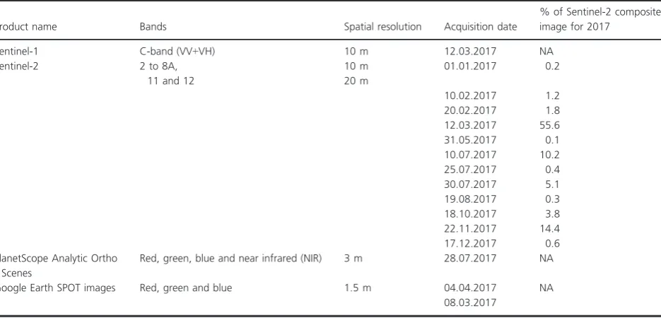
selecting cloud free areas from the various dates. We used 12 images in total (Table 1), and there was still 6.3% of the image left with no information due to persistent cloud cover in all the Sentinel-2 scenes available for 2017. The resulting composite image can be seen in Figure 3. Because the largest part of the composite Sentinel-2 image (>55%) comes from the scene acquired on the 12th of March 2017, we chose a Sentinel-1 scene with the same acquisition date (Table 1).

Reference data and definition of land cover classes

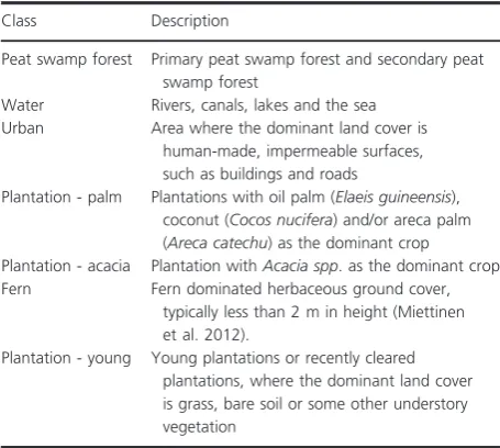
The classes used throughout this study (Table 2; Data S1) were chosen to represent the most common land cover types in the region (Miettinen and Liew 2010). The areas of fern are regrowth left unmanaged after severe fires. Whilst areas that have been subject to low-intensity fire undergo succession to secondary forest, high intensity or frequent fires degrade peatland to the extent that succes-sion back to forest is prevented. These areas undergo ret-rogressive succession to lower growing, less structured plant communities dominated by ferns, with very few trees (Page et al. 2009). The different species of palm (betel nut, coconut and oil palm) were considered as a single class because it was not possible to distinguish them from each other on the very high resolution images available. There are also areas of traditional rubber

agroforestry in the region (Ekadinata and Vincent 2011), but these represent only a small proportion of the study area and distinguishing these from peat swamp forest was beyond the scope of this study.

We collected the reference data through visual interpre-tation of very high resolution imagery, namely a PlanetS-cope scene from the 28th of July 2017 with a spatial resolution of 3 m (Planet Team 2017) and, where avail-able, higher resolution images for 2017 from Google Earth. The Google Earth images we used were SPOT images (sourced from DigitalGlobe), with a spatial resolu-tion of approximately 1.5 m.

We used the same reference dataset for all the classifi-cations in this study, made up of 1400 training points and 2800 test points, divided equally between the seven classes. We ensured that the reference data were well dis-tributed throughout the scene (Data S2) and only selected areas that we were confident we could identify. In addi-tion to this, because the optical image is a composite from various dates, we took the training and test points from all the imagery dates used, proportionally to the area they occupy in the final composite scene. This is based on the previous work that found that decision tree classification accuracy is not highly dependent on whether histogram match was used to make the composite ima-gery, provided that the training data are well distributed to include all the imagery dates and thus reflect class spectral variability (Helmer and Ruefenacht 2007). Table 1. Overview of the Sentinel-1, Sentinel-2, PlanetScope and Google Earth images used in this study. We used the Sentinel-2 images to cre-ate a single composite scene for 2017, displayed in Figure 3. It should be noted that 6.3% of the composite image has no information, due to persistent cloud cover in all available Sentinel-2 images for 2017.

Product name Bands Spatial resolution Acquisition date

% of Sentinel-2 composite image for 2017

Sentinel-1 C-band (VV+VH) 10 m 12.03.2017 NA

Sentinel-2 2 to 8A,

11 and 12

10 m 20 m

01.01.2017 0.2

10.02.2017 1.2

20.02.2017 1.8

12.03.2017 55.6

31.05.2017 0.1

10.07.2017 10.2

25.07.2017 0.4

30.07.2017 5.1

19.08.2017 0.3

18.10.2017 3.8

22.11.2017 14.4

17.12.2017 0.6

PlanetScope Analytic Ortho Scenes

Red, green, blue and near infrared (NIR) 3 m 28.07.2017 NA

Google Earth SPOT images Red, green and blue 1.5 m 04.04.2017

08.03.2017

Classification

We used three different approaches to map land cover: a pixel-based classification using OPVs, an object-based classification, and a pixel-based classification using PCs. For each approach we compared the results from data fusion (using the composite Sentinel-2 scene with a single Sentinel-1 scene from March 2017) with the use of a sin-gle data source (the composite Sentinel-2 scene on its own, or a single Sentinel-1 scene from March 2017 on its own).

We used a Random Forest classifier in all three approaches as it has demonstrated robust performance in land cover studies using diverse remote sensing datasets (Gislason et al. 2006; Waske and Braun 2009; Stefanski et al. 2013). We used the package randomForest (version 4.6-14; Liaw and Wiener 2002) in the R environment (R Core Team 2017). We set the parameter mtry to the default value (in this case 3) and ntree to 500, based on various trial runs and recommendations in the literature (Belgiu and Dragu 2016). In the case of the object-based classification, the features included in the Random Forest were mean and standard deviation of the objects for each layer in the stack.

We used the open source image segmentation tool in GRASS 7.0.5 (i.segment; Momsen and Metz 2017) to create objects and associated summary statistics (i.segment.stats; Lennert 2017). The GRASS image segmentation tool uses a region growing and merging technique, in which all pixels are used as seeds and the similarity between segments and unmerged objects is used to determine which objects are merged. We set the threshold for merging at 0.01 and the minimum object size to five pixels, based on various trial runs.

For the pixel-based classification using PCs we applied standardized principal component analysis in the R envi-ronment, using the package ‘RStoolbox’ (version 0.1.10; Leutner and Horning 2017). We then used the PCs as predictors in the Random Forest classification. The num-ber of PCs included in the different classifications was decided upon through examination of the loadings and Figure 3. The map shows the composite 2017 Sentinel-2 image used throughout this study, displayed as a natural-colour (RGB) image. Note the inconsistencies in illumination visible in some areas of the image, due to the fact that the image is a mosaic from various dates. The areas marked as cloud cover (6.3% of the scene) are where information is unavailable due to persistent cloud cover in all available Sentinel-2 scenes for 2017.

Table 2. Description of the various classes used this study.

Class Description

Peat swamp forest Primary peat swamp forest and secondary peat swamp forest

Water Rivers, canals, lakes and the sea Urban Area where the dominant land cover is

human-made, impermeable surfaces, such as buildings and roads

Plantation - palm Plantations with oil palm (Elaeis guineensis), coconut (Cocos nucifera) and/or areca palm (Areca catechu) as the dominant crop Plantation - acacia Plantation withAcacia spp. as the dominant crop Fern Fern dominated herbaceous ground cover,

typically less than 2 m in height (Miettinen et al. 2012).

visual examination of the PCs. The classification using only optical data included 7 PCs, the classification using only radar data 2 PCs and the classification using data fusion 9 PCs.

We carried out an accuracy assessment for each classifi-cation in order to compare performance. We calculated overall accuracy (proportion of correctly classified cases) and class-specific producer’s and user’s accuracies for each classification. Producer’s accuracy is calculated as the number of correctly classified test points divided by the total number of test points of that class, and it represents how often a real feature on the ground is correctly shown on the classified map. User’s accuracy is calculated as the number of correctly classified test points divided by the total number of test points classified as that class, and it tells us how often the class on the map will actually be present on the ground (Congalton and Green 2009). We used McNemar’s test for paired-sample nominal scale data (Agresti 2002) to assess whether statistically signifi-cant differences exist between the classifications. This test is suitable to assess the performance of multiple classifica-tions that use the same test and training samples (Foody 2004) and has been applied widely in thematic map com-parison (Duro et al. 2012; Fu et al. 2017).

Results

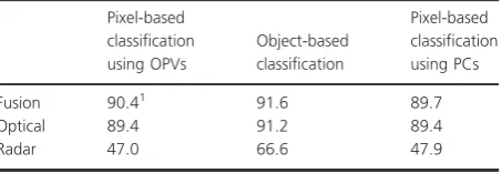
Data fusion increased overall accuracy by a statistically significant amount only in the case of the pixel-based classification using OPVs, compared to the use of only optical data (Table 3). In the case of the object-based classification and the pixel-based classification using PCs, fusion did not significantly increase overall accuracy com-pared to the use of only optical data. In all three meth-ods, fusion had a positive effect on some classes and a mixed or even negative effect on others (Data S3). The results from using only radar data showed comparatively low overall accuracy, but the object-based classification was the most promising results.

The object-based classification using data fusion had a significantly higher overall accuracy than the other two

approaches to fusion (P< 0.02 in both cases). It also had the highest user’s and producer’s accuracies for ‘forest’ and ‘acacia’, indicating its strength in discriminating these two classes (Table 4). Confusion between forest, plantation-palm and plantation-acacia was reduced with object-based classification, compared to the other two approaches (Data S5).

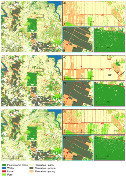
The land cover maps produced by data fusion using the three classification approaches can be seen in Fig-ure 4. All approaches detected the main rivers in the region, various urban centres and large industrial acacia plantations to the south and west of the protected area. Large swaths of the landscape were identified as palm plantations and a few discrete patches were identified as fern, including a large area in the south east of the study area. The resolution offered by the Sentinel data allowed many roads to be identified, mapped as either ‘urban’ or ‘plantation-young’. The canals, which often run parallel to roads, were not identified for the most part, presum-ably because the resolution of the imagery does not allow for it (even the largest canals in the region are typically less than 10 m across).

As can be seen in Figure 4, the object-based classifica-tion produced a map with less of the ‘salt and pepper’ effect seen in the other two approaches. This led to a more homogenous classification of the Sungai Buluh Pro-tection Forest (Figure 4 H) and acacia plantations (Fig-ure 4 G) for example, but also a loss of detail, such as smaller roads (Figure 4 F).

Discussion

Our results demonstrate that data fusion significantly improves our ability to map the loss of peat swamp for-ests in Southeast Asia within a pixel-based classification using OPVs, resulting in a 1% increase in overall racy. However, data fusion did not increase overall accu-racy in the object-based classification or the pixel-based classification using PCs, compared to the use of optical data only. The results also show that the object-based classification is associated with the best results in terms of accuracy, and produces a map with reduced speckle, although at the cost of a reduction in the detail of the mapping.

Those considering whether to use data fusion within a project might find the 1% increase in overall accuracy reported for the pixel-based approach using OPVs too low to warrant the additional pre-processing time and expertize required when radar data are used. The pre-pro-cessing steps for Sentinel-1 scenes do not require excessive computational time. It took us around 10 min to pre-process a Sentinel-1 scene following the steps described in the methods section. The use of fusion did not have a Table 3. Overall accuracy (%) for the different approaches to

classification. OPVs, original pixel values; PCs, principal components.

Pixel-based classification using OPVs

Object-based classification

Pixel-based classification using PCs

Fusion 90.41 _{91.6 89.7}

Optical 89.4 91.2 89.4

Radar 47.0 66.6 47.9

1

noticeable effect on the time it took to train the Random Forest classifier, which remained at around 30 sec when run on a desktop computer (6Core 2.60 GHz Processor, 56 Gb RAM and 446 GB of free hard drive space). How-ever, navigating the Sentinel-1 Toolbox and deciding on a pre-processing workflow can be daunting for those less familiar with radar data. There is thus a trade-off between the increase in accuracy when data fusion is used and the additional work involved.

Indeed, the results of the classification using the com-posite optical image on its own were surprisingly good considering the clear inconsistencies due to illumination differences between the 12 different dates used (Fig. 3). It may be that when faced with high cloud cover, project time is best spent creating as good a composite scene as possible and ensuring that reference data come from all the dates used, rather than processing and integrating radar data. The creation of the composite Sentinel-2 image took about 2 weeks to complete and was by far the most time-consuming step in this study. Any future improvements in the cloud detection algorithms available for Sentinel-2 images will increase automation, speed up this step and make it easier to scale up the method (Zhu et al. 2015).

The comparison of the three classification approaches highlights the strength of the object-based approach for our study area, even if only optical data are used. For those considering implementing it elsewhere, it is worth noting that in our study area the acacia plantations and peat swamp forest areas have large, clearly defined geo-metrical shapes, which might have made the landscape particularly well suited to an object-based classification. This approach is likely to be less suitable in areas where patterns are more subtle, and changes between land cover more gradual. In addition, the computational time was greater for the object-based classification than for the other two approaches. The tools implemented in GRASS GIS were comparatively slow and hampered by some problems with the GIS interface. The creation of segments and associated statistics for the study area took about

200 min, whilst running the Random Forest algorithm in R took less than 1 min, using data fusion and a desktop computer (6Core 2.60 GHz Processor, 56 Gb RAM and 446 GB of free hard drive space). The segmentation step also required more involvement from the user when selecting parameters. Thus, for anybody concerned with maximizing speed and automation, the best approach would be a pixel-based classification using OPV.

One of the limitations with the methods described in this paper is that the use of a composite Sentinel-2 scene with dates taken from throughout the year creates a risk of intra-annual land cover change. Clearance of forest for plantations and fires have been the key drivers of deforestation in the study area. However, there were no large fires in our study region in 2017 and the protected status of the Sungai Buluh forest means that degradation was minimal in 2017, even if it has not completely stopped. Thus the most likely rapid land cover change in the region is the harvest of acacia plantations. Whilst in our study area we can safely assume that intra-annual land cover change will not greatly affect our results, in regions where large areas of peat swamp forest are being removed within a year it would be more problematic to use a composite optical image with dates from through-out the year.

The best method for a mapping project depends to a great extent on the land cover dynamics in the study area, but also on how the information will be used. Land cover maps can support a range of decision-mak-ing in a conservation context, such as helpdecision-mak-ing identify suitable sites for peatland restoration (Graham et al. 2017). In our study site, for example, the areas of fern are of particular interest for restoration work because they are not economically productive and need tree planting, alongside hydrological restoration, if they are to return to a peat swamp forest (Page et al. 2009). Because of this, maps that identify these areas of fern reliably are of interest to understand their local context and degree of connectivity with other areas of forest, in order to assess how suitable they are for restoration. The Table 4. Producer’s and user’s accuracies (%) for forest, plantation-acacia and plantation-palm, resulting from the three different approaches to fusion.

Pixel-based classification using

OPVs Object-based classification

Pixel-based classification using PCs

Producer’s Accuracy

User’s Accuracy

Producer’s Accuracy

User’s Accuracy

Producer’s Accuracy

User’s Accuracy

Peat swamp forest 84.8 87.4 90.8 94.8 85.3 86.8

Plantation - palm 86.8 75.9 89.3 82.5 83.5 74.6

Plantation - acacia 78.3 91.8 80.5 89.2 75.3 88.8

fact that composite optical scenes can be used on their own to reliably map peat swamp forest loss also means that long-term studies of land cover change are possible in our study region, as medium resolution, open access optical data is available from the 1980s onwards thanks to the Landsat data policy (Wulder et al. 2016). These long-term studies on land cover change can provide important information on past patterns of peat swamp forest loss and speed of recovery.

Conclusion

Our work mapping deforestation in tropical areas with high cloud cover highlights that optical data are still the main source of information for classification purposes and that using radar data on its own does not produce good results. Fusion of optical and radar data did not increase overall accuracy in the case of the object-based classification or the pixel-based classification using PCs, and led to a small (but statistically significant) improve-ment in accuracy in the case of the pixel-based classifica-tion using OPVs, compared to the use of only optical data. This means that it is important to balance the gains in accuracy from fusion against the extra time needed to preprocess the radar data and incorporate it into the workflow of the mapping project.

This study applies data fusion and machine learning techniques to map peat swamp forest loss, and as such continues the work towards automated regional level mapping in Southeast Asia (Miettinen et al. 2017). The main barrier to scaling up the methods described in this paper is the technique used to create the composite opti-cal scene, as the cloud probability raster in the Sentinel-2 Level 2A products was not good enough to be used as a cloud mask. Multi-temporal approaches to cloud detec-tion are being developed to mask cloud (Hagolle et al. 2010; Mateo-Garcıa et al. 2018) and more work needs to be done to test their functionality in areas with very high cloud cover, adapt them for use with Sentinel-2 data and make the algorithms more accessible to a wider commu-nity of users. Traditionally, low computational power has limited those working in smaller institutions and NGOs, making it hard to map large areas and work with meth-ods that rely on time-series analysis. However, this has changed thanks to the availability of services such as the cloud-based platform Google Earth Engine (Gorelick et al. 2017) and the free virtual machines provided by the European Space Agency’s Research and User Support Ser-vice (RUS 2018). There is currently a growing interest in the potential of big data (Liu et al. 2018), which in a remote sensing context refers to the recent increase in the volume and variety of remote sensing data available, as well as the increase in processing velocity (Chi et al.

2016). These developments in online platforms and vir-tual machines should help those working in conservation to capitalize on the potential of big data to monitor large areas.

With conversion of tropical peatland to agriculture projected to continue (Wijedasa et al. 2018), long-term and large-scale monitoring of tropical peat swamp forests will remain relevant in the coming years. Knowledge about land cover and how it is changing in peatland areas will support restoration projects by giving them the infor-mation they need to identify suitable sites for restoration work, understand connectivity in the landscape and link fieldwork to the wider landscape.

Acknowledgments

We would like to thank Planet for providing us with Planet Scope Scenes free of charge through their Education and Research Program. We would also like to thank Anny Mulyani for her comments on the manuscript. This research was funded through the Newton Fund project “Enhancing the benefits of tropical peatland restoration for supporting local communities and ecosystem processes”, NERC Reference: NE/P014658/1.

Data Accessibility

The code used in this publication is freely available on GitHub: https://github.com/merrycrowson/fusion_optical_ radar.git.

The satellite remote sensing data used in the analysis can be downloaded for free from the Sentinel Open Hub (https://scihub.copernicus.eu/).

References

Agresti, A. 2002.Categorical Data Analysis. John Wiley and

Sons, https://doi.org/10.1198/tech.2003.s28.

Belgiu, M., and L. Dragu. 2016. Random forest in remote

sensing: a review of applications and future directions. ISPRS J. Photogramm. Remote Sens.114, 24–31.

Chi, M., A. Plaza, J. A. Benediktsson, Z. Sun, J. Shen, and Y. Zhu. 2016. Big data for remote sensing: challenges and

opportunities.Proc. IEEE104, 2207–2219.

Chisholm, R. A., L. S. Wijedasa, and T. Swinfield. 2016. The need for long-term remedies for Indonesia’s forest fires. Conserv. Biol.30, 5–6.

Congalton, R. G., and K. Green. 2009.Assessing the accuracy of

remotely sensed data: principles and practices, 2nd ed.. CRC Press/Taylor & Francis, Boca Raton.

Dohong, A., A. A. Aziz, and P. Dargusch. 2017. A review of the drivers of tropical peatland degradation in South-East

Asia.Land Use Policy69(October), 349–360.

Duro, D. C., S. E. Franklin, and M. G. Dube. 2012. A

comparison of pixel-based and object-based image analysis with selected machine learning algorithms for the

classification of agricultural landscapes using SPOT-5 HRG

imagery.Remote Sens. Environ.118, 259–272.

Ekadinata, A., and G. Vincent. 2011. Rubber agroforests in a changing landscape: analysis of land use/cover trajectories in

Bungo district, Indonesia.Forests Trees Livelihoods20, 3–14.

Foody, G. M. 2004. Thematic map comparison: evaluating the statistical significance of differences in classification

accuracy.Photogramm. Eng. Remote Sensing70, 627–633.

Fu, B., Y. Wang, A. Campbell, Y. Li, B. Zhang, S. Yin, et al. 2017. Comparison of object-based and pixel-based Random Forest algorithm for wetland vegetation mapping using high

spatial resolution GF-1 and SAR data.Ecol. Ind.73, 105–

117.

Gislason, P. O., J. A. Benediktsson, and J. R. Sveinsson. 2006.

Random Forests for land cover classification.Pattern Recogn.

Lett.27, 294–300.

Gorelick, N., M. Hancher, M. Dixon, S. Ilyushchenko, D. Thau, and R. Moore. 2017. Google Earth Engine:

planetary-scale geospatial analysis for everyone.Remote Sens. Environ.

202, 18–27.

Graham, L. L. B., W. Giesen, and S. E. Page. 2017. A common-sense approach to tropical peat swamp forest

restoration in Southeast Asia.Restor. Ecol.25, 312–321.

Hagolle, O., M. Huc, D. V. Pascual, and G. Dedieu. 2010. A multi-temporal method for cloud detection, applied to

FORMOSAT-2, VENlS, LANDSAT and SENTINEL-2

images.Remote Sens. Environ.114, 1747–1755.

Hapsari, K. A., S. Biagioni, T. C. Jennerjahn, P. M. Reimer, A. Saad, Y. Achnopha, et al. 2017. Environmental dynamics and carbon accumulation rate of a tropical peatland in

Central Sumatra, Indonesia.Quatern. Sci. Rev.169, 173–187.

Helmer, E. H., and B. Ruefenacht. 2007. A comparison of radiometric normalization methods when filling cloud gaps

in Landsat imagery.Can. J. Remote. Sens.33, 325–340.

Jaenicke, J., J. O. Rieley, C. Mott, P. Kimman, and F. Siegert. 2008. Determination of the amount of carbon stored in

Indonesian peatlands.Geoderma147151–158.

Joshi, N., M. Baumann, A. Ehammer, R. Fensholt, K. Grogan, P. Hostert, et al. 2016. A review of the application of optical and radar remote sensing data fusion to land use mapping

and monitoring.Remote Sens.8, 1–23.

Karger, D. N., O. Conrad, J. B€ohner, T. Kawohl, H. Kreft, R. W.

Soria-Auza, et al. (2016). CHELSA climatologies at high resolution for the earth’s land surface areas (Version 1.2). World Data Cent. Clim. https://doi.org/10.1594/wdcc/chelsa_v1_1 Lennert, M. (2017). GRASS Image Segmentation Statistics.

Available from https://grass.osgeo.org/grass74/manuals/add ons/i.segment.stats.html

Leutner, B., and N. Horning. (2017). RStoolbox: Tools for Remote Sensing Data Analysis. R package version 0.1.10. Available from https://cran.r-project.org/package= RStoolbox

Liaw, A., and M. Wiener. 2002. Classification and regression

by randomForest.R. News2, 18–22.

Liu, P., L. Di, Q. Du, and L. Wang. 2018. Remote sensing big data:

theory, methods and applications.Remote Sens.10, 2016–2019.

Mateo-Garcıa, G., L. Gomez-Chova, J. Amoros-Lopez, J.

Munoz-Mar~ ı, and G. Camps-Valls. 2018. Multitemporal cloud

masking in the Google Earth Engine.Remote Sens.10, 7–9.

Miettinen, J., and S. C. Liew. 2010. Status of peatland degradation and development in Sumatra and Kalimantan. Ambio39, 394–401.

Miettinen, J., A. Hooijer, C. Shi, and D. Tollenaar. 2012. Extent of industrial plantations on Southeast Asian peatlands in 2010 with analysis of historical expansion and

future projections.Glob. Change Biol. 908–918. https://doi.

org/10.1111/j.1757-1707.2012.01172.x

Miettinen, J., C. Shi, and S. C. Liew. 2016. Land cover distribution in the peatlands of Peninsular Malaysia,

Sumatra and Borneo in 2015 with changes since 1990.Glob.

Ecol. Conserv.6, 67–78.

Miettinen, J., C. Shi, and S. C. Liew. 2017. Towards automated 10-30 m resolution land cover mapping in insular Southeast

Asia.Geocarto Int.1–36. https://doi.org/10.1080/10106049.

2017.1408700

Momsen, E., and M. Metz. (2017). GRASS GSoC 2012 Image Segmentation. Available from https://grass.osgeo.org/gra ss74/manuals/i.segment.html

Moreira, A., P. Prats-Iraola, M. Younis, G. Krieger, I. Hajnsek, and K. P. Papathanassiou. 2013. A tutorial on

synthetic aperture radar.IEEE Geosci. Remote Sens. Mag.1,

6–43.

Murray, N. J., D. A. Keith, L. M. Bland, R. Ferrari, M. B. Lyons, R. Lucas, et al. 2018. The role of satellite remote

sensing in structured ecosystem risk assessments.Sci. Total

Environ.619–620, 249–257.

Page, S. E., and A. Hooijer. (2016). In the line of fire: The

peatlands of Southeast Asia.Philos. Trans. R. Soc. B Biol.

Sci.,371, 20150176.

Page, S., A. Hosciło, H. W€osten, J. Jauhiainen, M. Silvius, J.

Rieley, et al. 2009. Restoration ecology of lowland tropical peatlands in Southeast Asia: current knowledge and future

research directions.Ecosystems12, 888–905.

Page, S. E., J. O. Rieley, and C. J. Banks. 2011. Global and regional importance of the tropical peatland carbon pool. Glob. Change Biol.17, 798–818.

Planet Team. (2017). Planet Application Program Interface: In Space for Life on Earth. San Francisco, CA. Available from https://api.planet.com

Posa, M. R. C., L. S. Wijedasa, and R. T. Corlett. 2011. Biodiversity and conservation of tropical peat swamp

R Core Team. (2017). R: A language and environment for statistical computing. Vienna, Austria: R Foundation for Statistical Computing. Available from https://www.r-project.org/

Ritzema, H., S. Limin, K. Kusin, J. Jauhiainen, and H. W€osten.

2014. Canal blocking strategies for hydrological restoration of degraded tropical peatlands in Central Kalimantan,

Indonesia.Catena114, 11–20.

RUS. (2018). Copernicus Research and User Support (RUS) Service portal. Available September 11, 2018, from https:// rus-copernicus.eu/portal/

Schulte to B€uhne, H., and N. Pettorelli. (2018). Better together:

integrating and fusing multispectral and radar satellite imagery to inform biodiversity monitoring, ecological research

and conservation science.Methods Ecol. Evol.9, 849–865.

SNAP (2017). ESA Sentinel Application Platform. Version 6.0.0. http://step.esa.int.

Stefanski, J., B. Mack, and B. Waske. 2013. Optimization of object-based image analysis with random forests for land

cover mapping.IEEE J. Select. Topics Appl. Earth Obs.

Remote Sens.6, 2492–2504.

Waske, B., and M. Braun. 2009. Classifier ensembles for land

cover mapping using multitemporal SAR imagery.ISPRS J.

Photogramm. Remote Sens.64, 450–457.

Wetlands International. (2003). Peta-peta sebaran lahan gambut, luas dan simpanan/kandungan karbon di Sumatra (Maps of peatland distribution and carbon content in Sumatra), 1990-2002. Available from https://indonesia.wetla nds.org/publications/peatland-distribution-in-sumatra-and- kalimantan-explanation-of-its-data-sets-including-source-of-information-accuracy-data-constraints-and-gap/

Wijedasa, L. S., S. Sloan, S. E. Page, G. R. Clements, M. Lupascu, and T. A. Evans. 2018. Carbon emissions from Southeast Asian peatlands will increase despite emission

reduction schemes.Glob. Change Biol.24, 4598–4613.

World Bank. (2016). The Cost of Fire: An economic analysis of Indonesia’s 2015 Fire Crisis. Indonesia Sustainable

Landscapes Knowledge Note 1, 1–16. Available from http://

documents.worldbank.org/curated/en/776101467990969768/

pdf/103668-BRI-Cost-of-Fires-Knowledge-Note-PUBLIC- ADD-NEW-SERIES-Indonesia-Sustainable-Landscapes-Knowledge-Note.pdf

Wulder, M. A., J. C. White, T. R. Loveland, C. E. Woodcock, A. S. Belward, W. B. Cohen, et al. 2016. The global Landsat

archive: status, consolidation, and direction.Remote Sens.

Environ.185, 271–283.

Zhu, Z., S. Wang, and C. E. Woodcock. 2015. Improvement and expansion of the Fmask algorithm: cloud, cloud shadow, and snow detection for Landsats 4-7, 8, and

Sentinel 2 images.Remote Sens. Environ.159, 269–277.

Supporting Information

Additional supporting information may be found online in the Supporting Information section at the end of the article.

Data S1: Examples of the land cover classes used in the study. All of the photos were taken in, or very close to, the study area during July 2018. Photos by Merry Crow-son.

Data S2: Spatial distribution of the test and training data used in this study. The areas marked as cloud cover (6.3% of the scene) are where information is unavailable due to persistent cloud cover in all available Sentinel-2 scenes for 2017.

Data S3:Increase or decrease in producer’s accuracy (PA) and user’s accuracy (UA) for each class when fusion is used compared to optical only with (A) the pixel-based classification using the OPV, (B) object-based classifica-tion and (C) pixel-based classificaclassifica-tion using PCs.

Data S4: Producer’s and user’s accuracies (%) resulting from the three different approaches to fusion.