Working Paper Research
The Taylor principle and (in-)determinacy
in a New Keynesian model with
hiring frictions and skill loss
by Ansgar Rannenberg
Editorial Director
Jan Smets, Member of the Board of Directors of the National Bank of Belgium
Statement of purpose:
The purpose of these working papers is to promote the circulation of research results (Research Series) and analytical studies (Documents Series) made within the National Bank of Belgium or presented by external economists in seminars, conferences and conventions organised by the Bank. The aim is therefore to provide a platform for discussion. The opinions expressed are strictly those of the authors and do not necessarily reflect the views of the National Bank of Belgium.
Orders
For orders and information on subscriptions and reductions: National Bank of Belgium, Documentation - Publications service, boulevard de Berlaimont 14, 1000 Brussels. Tel +32 2 221 20 33 - Fax +32 2 21 30 42
The Working Papers are available on the website of the Bank: http://www.nbb.be.
© National Bank of Belgium, Brussels
All rights reserved.
Reproduction for educational and non-commercial purposes is permitted provided that the source is acknowledged. ISSN: 1375-680X (print)
Abstract
We introduce skill decay during unemployment into Blanchard and Gali's (2008) New-Keynesian model with hiring frictions and wage rigidity. Plausible values of quarterly skill decay and real-wage rigidity turn the long-run marginal cost-unemployment relationship positive in a "European" labour market with little hiring but not in a fluid "American" one. If the marginal cost-unemployment relationship is positive, determinacy requires a passive response to inflation in the central bank's interest feedback rule if the rule features only inflation. Targeting steady state output or unemployment helps to restore determinacy.
Under indeterminacy, an adverse sunspot shock increases unemployment extremely persistently.
Key Words: E24, E52, E32, J64.
JEL Classification: Monetary policy rules, Taylor principle, Determinacy, Hysteresis, Skill decay.
Corresponding author:
Ansgar Rannenberg, Research Department, NBB - e-mail: ansgar.rannenberg@nbb.be.
I am grateful for helpful comments from Gregory de Walque, Charles Nolan, Andrew Hughes Hallett, George Evans and Alan Sutherland. The usual disclaimer applies. I am grateful for generous financial support from the Centre for Dynamic Macroeconomic Analysis (CDMA) at the School of Economics and Finance at the University of St. Andrews.
TABLE OF CONTENTS
1. Introduction... 1
2. The Model ... 3
2.1 Households ... 3
2.2 Firms ... 4
3. Marginal Cost and Unemployment in the Presence of Skill Loss ... 11
4. Determinacy ... 17
4.1 Calibration of Non-Policy Parameters ... 18
4.2 Skill Decay and the Merits of an active Response to Inflation ... 21
4.3 How to restore Determinacy under the European Calibration ... 25
5. Dynamics under Indeterminacy ... 29
6. Conclusion ... 32
References ... 34
A Steady State Values and reduced Form Coefficients ... 41
B Proof of Proposition 1 ... 41
C Proof of Propositions 2 ... 42
D Model Equations in the Form required by Sims' (2000) Code ... 44
E Derivation of the Laws of Motion of and ... 49
F Derivation of the marginal Cost Equation and the Output Equation in the Model with Skill Loss ... 54
G Tables ... 58
H Figures ... 62
1
Introduction
The Taylor principle states that, in response to an increase in in‡ation, the central bank
should eventually increase the nominal interest rate more than one for one. The conventional
wisdom in monetary economics says that, to ensure a unique and stable equilibrium, monetary
policy should follow the Taylor principle. We show that an active monetary policy may
instead induce indeterminacy if unemployed workers lose a fraction of their skills per quarter
of unemployment, the real wage responds only imperfectly to changes in the worker’s skill
level, and labour market ‡ows are low.
The framework we develop adds skill decay during unemployment along the lines of
Pis-sarides (1992) to the New Keynesian model with hiring frictions and real-wage rigidity of
Blanchard and Gali (2008). In this environment, the marginal cost-unemployment
rela-tionship turns from negative to positive if quarterly skill decay and real-wage rigidity are
su¢ ciently high. Plausible values of quarterly skill decay and real-wage rigidity generate
a positive long-run marginal cost-unemployment relationship if the job …nding probability
is calibrated to the OECD-European median. This change in sign a¤ects the determinacy
requirements on the interest feedback rule of the central bank: A positive long- run marginal
cost-unemployment relationship almost always requires a coe¢ cient on in‡ation less than
unity if the central bank responds only to in‡ation. This does not depend on whether the
central bank responds to current, expected future, or lagged in‡ation. The reason appears
to be that with a positive long-run marginal cost-unemployment relationship, a persistent
increase in unemployment will ultimately increase marginal cost and thus in‡ation. If the
inter-est rate, subsequently lowering demand and thus validating the increase in unemployment:
Hence there is a self-ful…lling prophecy. The response of the economy to an adverse sunspot
shock con…rms this intuition.
By contrast, for a high "American" calibration of the job-…nding probability, the long-run
marginal cost-unemployment relationship never becomes negative for plausible values of skill
decay even if the real wage is perfectly rigid. Correspondingly, a coe¢ cient on in‡ation larger
than one guarantees determinacy.
Furthermore, adding the output gap to the policy rule solves the determinacy problem
under the "European" calibration if the central bank targets steady state output. Adding
unemployment has a similar e¤ect. By contrast, targeting ‡exible price output decreases the
determinacy region further if skill decay and real- wage rigidity are such that the long-run
marginal cost-unemployment relationship is positive.
Our results extend an evolving literature arguing that an active monetary policy may
induce indeterminacy if the interest rate set by the central bank has some indirect or direct
e¤ect on marginal cost. Such a channel may arise because the interest rate a¤ects capital
accumulation, job creation in models with matching frictions, or the cost of working capital
needed to fund the wage bill. In such environments, some upper bound on the in‡ation
coe¢ cient in the interest feedback rule is frequently necessary to ensure determinacy if the
central bank responds only to expected in‡ation, while responding to current in‡ation is still
stabilising.1 A notable exception is Christiano et al. (2010), who …nd that under reasonable
calibrations, even an active response to current in‡ation induces indeterminacy if …rms use
1Examples are Kurozumi and van Zandweghe (2008a), Carlstrom and Fuerst (2005) and Du¤y and Xiao
their own …nal output as an input and have to borrow to pay in advance a fraction of their cost
of labour and materials. However, the typical …nding in the literature is that the determinacy
problem is caused by the timing subscript of in‡ation in the interest feedback rule but not
by the active response to in‡ation per se. By contrast, in the model developed below, it is
the Taylor principle itself— the idea that an increase in in‡ation should sooner or later cause
an increase in the real interest rate— which creates scope for self-ful…lling prophecies.
The remainder of the paper is structured as follows. Section 2 derives the model. Section
3 shows how the long-run e¤ect of a permanent increase in unemployment on marginal cost is
a¤ected by the introduction of skill decay. Section 4 explores the conditions for determinacy
and how they are a¤ected by skill decay. Section 5 discusses the response of the model under
the European calibration to an adverse sunspot shock. Section 6 concludes.
2
The Model
2.1
Households
The economy is populated by a continuum of in…nitely lived households. A household consists
of a continuum of members who may be employed or unemployed but are all allocated the
same level of consumption. The households periodtincome derives from total wage payments
W Pt earned by the employed members, nominal interest payments it 1 on holdings of a
of consumption goods Ct and the risk-less bond Bt to maximise
Et
1
X
t=0
logCt
subject to the budget constraint
W Pt+ Bt 1
Pt
(1 +it 1) +Ft Ct+
Bt Pt
where Pt andNt denote the price level of the CES basket and hours worked by the members
of the household, respectively.
2.2
Firms
There are two types of …rms. Final goods …rms indexed by i produce the varieties in the
CES basket of goods consumed by households. They use the intermediate goodXt(i)in the
linear technology
Yt(i) = Xt(i)
The demand curve for varietyiresulting from the household spreading its expenditures across
varieties in a cost minimising way is given by ct(i) = Ct pt(i)
Pt ; where ct(i); pt(i) and Pt
denote consumption and price of variety i and the price level of the consumption basket,
respectively. Final goods …rms face nominal rigidities in the form of Calvo (1983) contracts,
They accordingly maximise
Et " 1
X
i=0
(! )i Ct
Ct+i Ct+i
"
pt(j) Pt+i
1
mct+i
pt(j) Pt+i
##
wheremctdenotes real marginal costs. The price level evolves according toPt1 = (1 !) (pt(j))
1
+
!(Pt 1)1 ; where pt(j) denotes the price set by those …rms allowed to reset their price in
period t.
The intermediate goods …rms employ labour to produce intermediate goods Xt(j).
In-termediate goods …rms operate under perfect competition and are owned by households. A
…xed fraction of jobs is destroyed each period. Thus employment of …rmj evolves
accord-ing to Nt(j) = (1 )Nt 1(j) +Ht(j) whereHt(j) denotes the amount of hiring in …rm j.
Aggregate hiring is accordingly given by
Ht =Nt (1 )Nt 1 (1)
Note that the lower is ; the more Ht will depend on the change as opposed to the level of
employment. The number of job seekers at the beginning of the period is de…ned as Ut. Ut
consists of those workers who did not …nd a job at the end of period t 1 and those whose
jobs were destroyed at the beginning of t:
Ut= 1 Nt 1+ Nt 1 = 1 (1 )Nt 1 (2)
proportional to the productivity of a newly hired worker
Gt=AtB0xt (3)
where Atdenotes the average productivity of newly hired workers, to be de…ned below, B0 is
a constant, and xt denotes labour market tightness, de…ned as the ratio between aggregate
hiring Ht and Ut:
xt= Ht Ut
(4)
The intuition behind(3) is that if hiring is high relative to the number of job seekers, it takes
on average longer to …ll a vacancy. Since posting a vacancy is costly, hiring costs increase in
xt:2 We interpret labour-market tightness xt as the probability of an unemployed person to
move into employment in period t.
Following Pissarides (1992), we assume that the productivity of a newly hired worker is
the product of exogenous technology AP
t and his skill level. An unemployed worker loses a
fraction s 2[0;1] of his skill per quarter of his unemployment spell. Hence the skill level of
a worker with unemployment spell i is denoted by is, where s = 1 s and s 2[0;1] . i
equals zero if the newly hired worker lost his previous job in period t, one if he lost his job
in period t 1, and so on. Thus the productivity of a worker with unemployment duration
i is given by AP t
i s:
We assume further, following Pissarides (1992), that the unemployed regain all their skills
after one quarter of employment, that when intermediate goods …rms make the decision
2Hence equation (3) can be viewed as a short cut to a model which would specify a matching function
whether to hire or not and thus pay the hiring cost Gt; they know the state of exogenous
technologyAP
t but not the type of worker with whom they are going to be matched and that
they meet workers according to the share of these workers among job seekers.3 Furthermore,
for simplicity, we assume that a …rm does not hire individual workers, but only a group of
workers su¢ ciently large for the distribution of skills in the group to match the distribution
of skills in the job seeking population Ut. This ensures that the average skill level of the
group hired by the …rm equals the average skill level in the job seeking population.4
We denote the average skill level in the job seeking population as AL
t; implying that the
average productivity of newly hired workers is given by
At=APt A L
t (5)
while ALt is given by
ALt = 1
X
i=0
i ss
i
t (6)
where si
t denotes the share of those unemployed i periods among job seekers. Note that
AL
t < 1 if s >0 while for s = 0; we have s = ALt = 1: The shares of the various types of
workers among the total number of job seekers Ut is denoted as sit;and is de…ned by
sit=
Nt i 1
i
j=1(1 xt j) Ut
(7)
Note that Nt i 1 represents all those workers who had a job in periodt i 1but lost it
3See Pissarides (1992), pp. 1371-1391.
4This assumption rules out the possibility that, after paying the hiring cost, a …rm meets an individual
in period t i;while i
j=1(1 xt j)represents the fraction of those workers laid o¤ in period t iwho are still unemployed at the end of periodt 1:Hence the numerator consists of all
workers laid o¤ in period t iand still unemployed in period t 1:
As in Blanchard and Gali (2008), who in turn follow the seminal contribution of Hall
(2005), we assume that the real wage of a worker is rigid. The wage Wti of a worker who
has been unemployed for i periods is given by Wi t = 0
i s
1
AP t
1 P
; with 0 1
and 0 P 1: Hence for > 0 or P > 0 an increase in the worker’s skill level or an
increase in technology will cause a less-than-proportional increase in his real wage. While the
degree of real-wage rigidity with respect to technology P does not actually matter for the
determinacy results which are the subject of this paper, the degree of rigidity with respect to
the workers skill level will have an e¤ect. By assumption, Hall’s (2005) "…xed wage rule",
as well as Blanchard and Gali’s real wage schedule, lies always inside the bargaining set.
This implies that it neither prevents the formation of matches with a positive surplus nor
results in ine¢ cient separations.5 Under our assumption that …rms are restricted to hiring a
representative sample of job seekers, this condition is satis…ed in our model as well.
Hall (2005) interprets his constant wage rule as a social norm along the lines of Bewley
(1998,1999), who forms part of a growing literature arguing that employers are reluctant to
lower real wages and, what is more, to pay lower wages to newly hired employees than to
their existing workforce because doing so would hurt morale and thus productivity.6 Hence
the evidence suggests that employers will likely not adjust the wage of a new hire in full
5See Hall (2005), p.56.
6See Fabiani et al. (2010), pp. 501-502 and Galušµcák et al. (2010), p. 11-12. Similar survey results are
proportion to the loss in productivity induced by his unemployment duration, i.e. will be
positive. We will consider a wide range of values for this parameter in section 4.
The average real wage of the group the …rm hires is given by
Wt = 0
1
X
i=0
i(1 )
s s
i t
!
APt 1 P
(8)
0 is backed out to support a desired steady state combination of x; and N:This is shown
in appendix A. For future reference, we denote the skill dependent part of the average real
wage as
WtL = 1
X
i=0
i(1 )
s s
i t
!
(9)
The intermediate goods …rms will hire additional groups until the hiring cost of an
ad-ditional group equals the present discounted value of the pro…ts generated by this group.
However, unlike in the Blanchard and Gali model, we have to take into account the fact that
the skill level of the workforce hired in period t as well as their wage change in periodt+ 1.
This change arises because all hired workers who remain employed upgrade to the full skill
level after one quarter. Thus we have
Gt= PI
t Pt
APt ALt Wt+Et " 1
X
i=1
(1 )i iuC(Ct+i)
uC(Ct)
PtI+i Pt+i
APt+i Wt0+i
#
where PtI
Pt denotes the real price of intermediate goods while
i uC(Ct+i)
uC(Ct) denotes the stochastic
discount factor of the representative household.
The terms PtI
PtA
P
t ALt WtandEt " 1
X
i=1
(1 )i i uC(Ct+i)
uC(Ct)
PI t+i
Pt+iA
P
t+i Wt0+i #
represent the
discounted value of pro…ts generated in period t+ 1and after, respectively. Note that due to
our assumption that a worker regains all his skills after one period, the expression for the ‡ow
pro…t in periodt is di¤erent from the expression for the ‡ow pro…t in periodt+ 1and after.
Rewriting this equation as a di¤erence equation, noting that the real price of intermediate
goods …rms equals the marginal cost of …nal goods …rms (hence PtI
Pt =mct) and that with log
utility, uC(Ct+i)
uC(Ct) =
Ct
Ct+i, we have
mctAPtA L
t =Wt+Gt (10)
(1 )Et
Ct Ct+1
Gt+1+mct+1APt+1 W 0
t+1 mct+1APt+1A
L
t+1 Wt+1
The left-hand side represents the real marginal revenue product of labour, which depends
on the period t average skill level among applicants. Clearly, an increase in the quality of
the average period to job seeker AL
t will reduce periodt marginal cost. The right hand side
features the periodt real wageWtand the periodthiring costsGt, and, with a negative sign,
the present expected value of hiring costs saved (Gt+1) by hiring the group int rather than
t+ 1. While an increase in hiring cost today means increasing production is more costly, an
increase in future expected hiring costs will induce intermediate goods …rms to shift hiring
into the present, thus lowering the price of intermediate goods and thus marginal cost.
In addition, the right hand side also includes the present expected value of the t + 1
di¤erence between the real pro…t generated by a fully skilled group (with productivity APt+1
and real wage W0
t+1) and a t+ 1 newly hired group (with productivity APt+1ALt+1 and real
wage Wt+1). This represents an additional bene…t of hiring today rather than tomorrow
decreases in ALt+1 and increases in Wt+1 and mct+1: Thus an expected highert+ 1 skill level
will increase marginal cost in periodt (since it reduces the bene…t from hiring today), while
a higher expected average real wage for the t+ 1 newly hired and a higher expected t+ 1
price of intermediate goods (i.e. higher t+ 1 marginal cost) will decrease it.
The average productivity of the whole workforce after adding the newly hiredAA
t and the
production functions of gross outputYt(i.e. output including hiring costs) and consumption
goodsCtare then given by (where sNt denotes the share of the newly hired in the workforce)
AAt = APt sNt AtL+ 1 sNt , sNt = Ht
Nt
= Nt (1 )Nt 1
Nt
(11)
Yt = AAtNt (12)
Ct = AAtNt B0xtA P tA
L
tHt=AAtNt B0xtA P tA
L
t (Nt (1 )Nt 1) (13)
3
Marginal Cost and Unemployment in the Presence
of Skill Loss
Let us now characterize the long-run relationship between marginal cost and unemployment in
the presence of hiring frictions, skill decay and real-wage rigidity in order to build the intuition
for the e¤ects of skill decay on determinacy we will discuss in section 4. We will ignore the
state of technology in what follows since it does not matter for determinacy. Combining
of marginal cost from its steady state as a function of unemployment:
c
mct = aL1baLt +w1LwbLt +aL2EtbatL+1 wL2EtwbtL+1 hcEtmcct+1 (14)
h00
1 uubt
h0L
1 ubut 1
h0F
1 uEtbut+1
where aL1; aL2; w1L; w2L; p0; p1; h
0
0; hc >0; h
0
L; h
0
F <0
b
aLt = 1
X
i=1
auiubt i; ani >0 (15)
b
wLt = 1
X
i=1
wuiubt i; wni >0 (16)
A lower case variable with a hat denotes the percentage deviation of the respective upper case
variable from its steady state, with the exception of ubt, which denotes the percentage point
deviation of unemployment from its steady state. The de…nitions of the various coe¢ cients
are displayed in table 1. Note while the average skill level among job seekers in period t
b
aLt negatively a¤ects marginal cost, the period t + 1 average skill level EtbaLt+1 enters with
a positive sign because, as was discussed above, a higher average period t + 1 skill level
reduces the bene…t from hiring today rather than tomorrow and thus increases marginal
cost. Analogously, an increase in EtwbtL+1 lowers mcct:
It is easily shown that with no skill decay (i.e. for s= 0), we haveani =wni =baLt =wbtL=
hc = 0 and thus (14) collapses to the marginal cost equation in Blanchard and Gali (2008):
c
mct= h0
(1 u)but+
hL
(1 u)but 1+
hF
(1 u)Etubt+1 p0bat
where the coe¢ cients are exactly as in Blanchard and Gali (2008). Note that marginal
unem-ployment due to the e¤ect of unemunem-ployment on the cost of hiring an additional worker. A
decrease in but increases period t hiring and thus labour market tightness and the cost of
hiring. A decrease in ubt 1 lowers period t hiring for a givenbut and thus period t hiring cost.
A decrease Etbut+1 increases periodt+ 1 hiring and hiring cost, thus increasing the bene…t of
creating jobs today and correspondingly reducing marginal cost today. The e¤ects of lagged
and lead unemployment increase in absolute value as the job destruction rate falls since
this increases the e¤ect of past employment on current hiring and of current employment on
future hiring, respectively, as can be obtained from (1):Therefore, the e¤ect of a permanent
increase in unemployment on marginal cost becomes less negative as increases.
Never-theless, it always remains negative because the negative e¤ect of current unemployment on
marginal cost always dominates the positive e¤ects of lagged and lead unemployment, as
h0
(1 u)
hL (1 u)
hF (1 u) <0:
7
As we will see shortly, this is no longer always true in the presence of skill decay and
real-wage rigidity. Let us denote reductions of the skill level of the average job seeker and the
average real wage caused by a one percentage point increase in unemployment as au = P1 i=1
au i
and wu = P1
i=1
wui; respectively. The following proposition summarises the properties of these
reductions and their derivatives with respect to s and :
7This is easily shown: We want to prove that 1
1 u(h0+hL+hF)
= 1 1 u
gM 1 + (1 )2
(1 x) (1 ) (1 x) (1 ) > 0: Using the fact that that 1 =
N x
N(1 x), this can be simpli…ed to(1 N)x
2+ (N x)N(1 )>0:This holds for all permissible values of
Proposition 1 Let au = P1
i=1
aui and wu = P1
i=1
wiu the decline of the average skill level and
the average real wage, respectively, caused by a permanent one percentage point increase in
unemployment. Then it is possible to prove the following three results:
(i)au > wu >0if and only if >0and s >0:Intuition: An increase in unemployment
increases the share of workers with longer unemployment durations and -with skill decay
( s > 0)- lower skill levels and thus lower real wages in the job seeking population. If the
wage of a worker only imperfectly adjusts to movements in his individual skill level ( >0),
the average real wage of job seekers declines by a smaller percentage than their average skill
level.
(ii) @a@ u s >
@wu
@ s > 0 if s is close to 0 and > 0: Intuition: A higher s lowers the skill level of the long-term unemployed. Hence an increase in the share of the long-term
unemployed among job seekers causes a faster decline in the average skill level and the average
real wage if s is higher. Real-wage rigidity ( >0)implies that the the decline in the average
skill level is accelerated by more than the decline in the average real wage.
(iii) @wu
@ < 0 if and only if s > 0 and < 1: Intuition: The higher ; the lower the
response of a worker’s real wage to movements in his skill level. Hence the reduction in
the average real wage associated with an increase of the share of the long-term unemployed
de-accelerates.
Proof: Appendix B.
Hence in the presence of real-wage rigidity ( > 0) and positive skill loss ( s > 0) a
"permanent" increase in unemployment increases the ratio between the (average) wage of
the real wage and productivity increases in s and falls in :
Hence skill decay in combination with real-wage rigidity creates a channel via which a
permanent increase in unemployment increases marginal cost, the more so the higher s and
: One can see that more formally by writing the long-run marginal cost-unemployment
relationship as
c
mc = ub (17)
=
h00+h0L+h0F
(1 u) a
u aL
1 aL2 wu wL1 w2L
(1 +hc)
A detailed derivation can be found in appendix C. gives the e¤ect of a "permanent"
increase in unemployment on marginal cost. Most conveniently, substituting the de…nitions
of h00; h0L and h0F shows that h00+h0L+h0F exactly equals, h0+hL+hF and is thus always
positive and independent of s:Hence only the term in the squared brackets and hc actually
depend on skill loss.
The squared bracket encapsulates the "skill loss channel" from unemployment to marginal
cost. It will be zero if s= 0, implying that >0and thus a negative e¤ect of a "permanent"
increase in unemployment on marginal cost. The …rst term represents the decline of the skill
level of the average applicant caused by the increase in ub (au) times the net e¤ect of a
permanent skill level decline on marginal cost ( aL
1 aL2 ). The second term represents the
decline of the skill-dependent real wage caused by the increase in bu(wu) times the net e¤ect
of a permanent decline in the skill dependent real wage on marginal cost (- wL
1 wL2 ).
From table 1 we obtain aL
1 > aL2 and wL1 > w2L since the gain from hiring today rather
wL1 wL2 will be quite close for sensible calibrations. Proposition 1, then, would imply that
for positive s and the squared bracket is positive and increases in s and : Thus skill
decay and real-wage rigidity would indeed render the e¤ect of unemployment on marginal
cost less negative, the more so the higher s and :We con…rm this by proving the following
proposition:
Proposition 2 Let ; formally de…ned in (17); be the decline in marginal cost caused by
a permanent one percentage point increase in unemployment and let s close to zero. Then
@
@ s < 0 if >
B0x M (1 )
1 B0x M(1 (1 )).8 Furthermore, @@ < 0 if and only if s > 0, < 1
and x(1 ) + x(1 (1 ) )
(1 (1 x) 1s ) >(1 x) 1
1
s Proof: Appendix C.
The conditions under which @
@ s <0and
@
@ <0are easily ful…lled for the calibrations we
will adopt later.
Hence our model features two long-run e¤ects of unemployment on marginal cost. The
…rst is the "hiring cost channel" of Blanchard and Gail (2008) (i.e. h
0 0+h
0 L+h
0 F
(1 u) ) , which is
always negative but decreases as the job destruction rate and thus -at a given level of
employment- the job …nding probability x decrease. The second is the skill decay channel
(i.e. an aL1 aL2 wn wL1 w2L ) which arises if there is real-wage rigidity and skill decay.
It’s strength increases s if > 0 and in if s > 0: If the skill decay channel e¤ect
dominates the hiring cost channel, an increase in unemployment will increase marginal cost
and in‡ation. This has consequences for the determinacy properties of the interest feedback
rule of the central bank, as we show in the next section.
8A more general proof without restrictions on
s would have been desirable but struck us as impossible
due to the complexity of the expression resulting from @@
4
Determinacy
In this section we explore how the conditions for determinacy in the above model are shaped
by skill decay and real-wage rigidity. After discussing the calibration of the non-policy
parameters in section 4.1, we show in section 4.2 that if labour market ‡ows are low and
real-wage rigidity and skill decay are su¢ ciently high, responding more than one for one
to in‡ation induces indeterminacy. In section 4.3, we check the merit of several possible
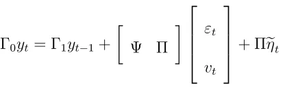
remedies for the indeterminacy problem. The linearised model consists of the following
equations (technology is again suppressed since it is irrelevant for determinacy):
t = Et t+1+ mcct (M1)
c
mct = a baLt +w wbtL 0ubt+ Lbut 1+ FEtbut+1 hcEt mcct+1 (M2)
b
aLt = (1 x) (1 s) ubt 1
u(1 u)+ sba
L
t 1 (M3)
b
wLt = (1 x) 1 1s but 1
u(1 u) +
1
s wb L
t 1 (M4)
b
ct = baPt +cLbatL c0but c1but 1 (M5)
b
ct = Etbct+1 bit Et t+1 (M6)
bit = Et t+j; 0; 1 j 1 (M7)
(M1) is the New Keynesian Phillips curve. (M3)and (M4) are merely quasi-di¤erenced
versions of(15) and (16): (M2)is the result of combining(M3)and (M4)with (14):(M5)
is derived by linearising equations (11) (13)and combining the resulting expressions.9 The
de…nitions of all reduced form coe¢ cients can be found in table 1. (M6) is the consumption
9Throughout we usebn
Euler equation while (M7) is the interest feedback rule of the central bank, which may be
current, forward or backward looking. Unfortunately, we cannot establish the conditions for
determinacy analytically.10 Therefore, we solve the model numerically using the software
Dynare.
4.1
Calibration of Non-Policy Parameters
The calibration is displayed in table 2. In line with the literature, we set = 0:99: Similar
to Blanchard and Gali, the steady state job …nding probability and unemployment rate x
and u are allowed to take two values, a high "American" and a low (OECD-) "European"
one. Hobijn and Sahin (2009) estimate average job …nding probabilities for advanced OECD
economies.11 For the United States, their (monthly) estimate corresponds to a quarterly
rate of 0.9.12 The median job …nding rate for the European countries included in Hobijn
and Sahin’s sample is 0.2, while the mean is 0.26. We set x = 0:2; which also happens to
equal their estimate for Germany and is very close to their estimate for France. Below we
will also show how our results are a¤ected by varying x between 0.2 and 0.9, covering both
Blanchard and Gali’s preferred calibrations ofxfor Europe and for the United States of 0.25
and 0.7, respectively, as well as Shimer’s (2005) estimate for the United States of 0.8. The
10In the absence of skill decay (
s= 0), it is possible to analytically establish the conditions for determinacy
for an interest feedback rule where the central bank responds only to in‡ation, as we show in Rannenberg (2009) by reducing it to a system of two jump variables and one predetermined variable and then applying conditions derived by Woodford (2003) for such systems. By contrast, with skill decay the model has three forward looking variables and three state variables. As far as we are aware, there is no straightforward way to analytically determine the eigenvalues of a 6x6 system.
11The countries inlcuded in the study are Australia, Austria, Belgium, Canada, Czech Republic, Denmark,
Finaland, France, Germany, Greece, Hungary, Iceland, Ireland, Italy, Japan, Luxembourg, Netherlands, New Zealand, Norway, Poland, Portugal, Slovak Republic, Spain, Sweden, Switzerland, United Kingdom and the United States.
12Hobijn and Sahin (2009) estimate a monthly job …nding rate x
m of 0.56. Following Blanchard and
Gali (2008), we convert their estimates into quarterly numbers using the formula x=xm+xm(1 xm) +
steady state unemployment rate u is set equal to 0.1 for Europe and to 0.05 for the United
States. Note, however, that for a given value of x; whetheru is set equal to 0.1 or 0.05 has
only marginal e¤ect on our results. The calibrated values of x and u imply the values for
displayed in the table.
We follow Blanchard and Gali (2008) in setting the parameters pertaining to the hiring
cost andB0 and the coe¢ cient on marginal cost in the Phillips curve :A value of = 1 is
consistent with estimates of matching functions. SettingB0 = 0:12implies a fraction of hiring
costs in GDP of about one percent under the American calibration, and correspondingly a
lower fraction under the continental European calibration sincexis lower.13 = 0:08implies
that prices remain …xed on average for about four quarters.
Calibrating the degree of real-wage rigidity with respect to the individual skill level is
di¢ cult because we lack hard evidence. Hall (2005) assumes the real wage to be constant,
corresponding to = 1: The survey evidence we cited above suggests that …rms are highly
reluctant to pay lower wages to newly hired workers, so this value may well be adequate.
Blanchard and Gali (2008) simply set = 0:5 since it is the midpoint of the admissible
range. In order to obtain some guidance, we log and HP …lter data on real wages and labour
productivity for the United States and Germany from 1970q1 and 1991q4 and regress the
former on the later.14 The point estimate of the coe¢ cients on the log of productivity are 0.5
for the United States and 0.34 for Germany, respectively. If we impose the restriction = P;
13See Blanchard and Gali (2008), p.27.
14This follows Hagededorn and Mankowskii (2008), who use this procedure to obtain a target value for
i.e., assume that workers’ wages are equally in‡exible with respect to skill and technology,
this would roughly corresponds to values of of 0.5 and 0.66, respectively.15 However, since
the restriction = P might well be invalid and since the regression exercise probably takes
our simple model of wage formation a bit too seriously, we will allow to vary between zero
and one in every grid search conducted below.
For guidance on how to calibrate quarterly skill decay s we draw on the literature on
wage loss upon worker displacement. This literature has produced evidence based on panel
regressions showing that the wage upon reemployment depends negatively on the duration of
the unemployment spell. Skill decay during unemployment is usually seen as one of the factors
causing this relationship, although the evolution of the reservation wage due to other factors
(for instance, depletion of an unemployed person’s wealth) would be expected to play a role
as well. Evidence along these lines include Addison and Portugal (1989) for American male
workers, Pichelmann and Riedel (1993) for Austrian workers, Gregory and Jukes (2001) for
British male workers, Gregg and Tominey (2005) for male youths, and Gangji and Plasman
(2007) for Belgian workers. They …nd that a one-year unemployment spell reduces the real
wage by 39%, 24%, 11%, 10% and 8% respectively.16 Furthermore, Nickell et al. (2002),
15The correspondence between the elasticity of the average wage with respect to average productvity and
is not perfect, but very close in this case. Across all the calibrations we consider in this paper, the aggregate
elasticity is always slightly larger than :
16For Addison and Portugal (1989), we have calculated the annual earnings penalty using the lower
coef-…cient on log(duration) in their two preferred speci…cations (Table 3, columns 5 and 6), p. 294. Duration is measured in weeks. For Pichelmann and Riedel (1993), we had to resort to the same procedure, see p. 8 in that paper for the results. Their coe¢ cient estimates for the e¤ect on the real wage is reported in table 2, p. 8. The results of Gregory and Jukes (2001) are reported on page F619, while the results of Gangji and Plasman (2007) are reported on page 18, table 2.
looking at British male workers, asks how the earnings loss is changed if the unemployment
spell exceeded six months and …nd an additional permanent earnings loss between 6.8% and
10.6%.17 Based on these estimates we will allow
s to vary between 0 and 0.07 (step size:
0.005) in every grid search, implying that a one-year unemployment spell reduces a worker’s
skill level by between 0 and 25%.
Unless otherwise mentioned in this section or below, the stepsize used in the parameter
intervals of the gridsearches conducted below is always 0.1.
4.2
Skill Decay and the Merits of an active Response to In‡ation
We set = [0;3]. For the American calibration, we …nd that determinacy requires >1
for all values of skill decay s and real-wage rigidity we consider in the grid search, i.e.
following the Taylor principle guarantees a unique equilibrium. By contrast, > 1 is not
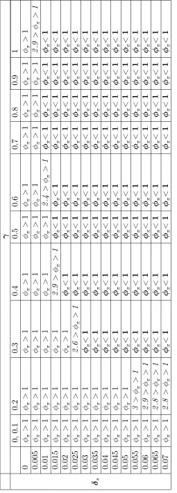
always su¢ cient to induce determinacy under the European calibration. Table 3 displays
the determinacy requirements on for the current looking rule for the values of s and
included in the gridsearch. While for very ‡exible real wages ( 0:1) > 1 is su¢ cient
for determinacy, for = 0:2 and s 0:055; starts being bounded above. What is more,
for = 0:3 and s 0:03; the determinacy requirement switches to < 1 : The central
bank now has to lower the real interest rate in response to an increase in in‡ation. Indeed,
for every value of larger or equal to 0.3, there exists a critical threshold value of s. If s
equals or exceed this value, determinacy requires a passive response to in‡ation. The critical
threshold value declines as increases. For instance, for = 0:5; the degree of real-wage
rigidity assumed by Blanchard and Gali (2008), the critical value of s equals 0.015, while
for 0:7 it is reduced to 0.01. The determinacy regions for the backward and forward
looking rules (not shown) are almost identical. In particular, the critical values of s are
identical across the three rules. This suggests that it is not the timing of the active response
to in‡ation but the active response to in‡ation per se which induces indeterminacy.
The critical values of s and the annual skill loss implied by these quarterly values are
displayed in table 4. The implied annual skill losses seem moderate compared with the
evidence on the e¤ect of unemployment duration on the reemployment wage cited in section
4.1.
To gain some intuition for why for some values of and s an active monetary policy is
destabilising under the European calibration, we draw on the long-run relationship between
marginal cost and unemployment. As discussed in section 3, this relationship is always
negative for s = 0 (i.e. >0) but becomes less so as s increases since @@s < 0 if there is
some real-wage rigidity. Indeed, as we increase s; may ultimately turn negative, implying a
positive marginal cost-unemployment relationship. However, under the American calibration,
never turns negative for the combinations of and s in our grid. By contrast, under the
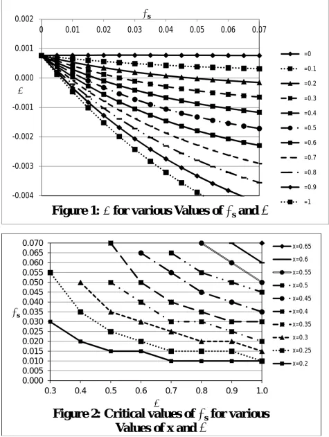
European calibration, does turn negative for some combination of and s:Figure 1 plots
against sfor the European calibration. Each line corresponds to a di¤erent value of :For
= 0; is essentially ‡at, while it decreases in s for 0:1: Furthermore, for any given
s > 0; higher values of are associated with lower values of ; as we would expect from
proposition 2.
never turns negative for 0:1: Hence never turns negative for those degrees of
real-wage rigidity for which is never bounded above. Furthermore, note that for 0:3,
equals this critical value of s: An intermediate case appears to be constituted by = 0:2 :
Here turns negative for s= 0:05but, as we saw above, the determinacy requirement does
not switch to <1; although becomes bounded above for s 0:055: However, by and
large, we can conclude that if marginal costs, and thus in‡ation, increase in response to a
persistent increase in the unemployment rate -because s exceeds the respective critical level
and thus we have < 0-, the central bank should lower the real interest rate to ensure a
unique equilibrium.
This prescription should rule out self-ful…lling prophecies. In response to a sunspot driven
persistent decrease in demand and increase in unemployment the central bank would increase
demand and hence would not validate the increase in unemployment. By contrast, with
1; there is scope for sunspot equilibria if s exceeds its respective critical value: A
persistent increase in unemployment will ultimately lead to an increase in in‡ation and (as
1) the real interest rate, irrespective of whether the central bank responds to lagged,
current or expected future in‡ation. This lowers demand and thus validates the increase
in unemployment. In the next section, when we display the impulse response function to a
sunspot shock, we show that this is in fact exactly what happens.
This leaves the question why this critical value is so much higher for the American than for
the continental European calibration. The chief reason for this is that due to the more ‡uid
labour market associated with the American calibration, for any combination of and s;
is a lot higher than under the continental European calibration. The intuition for that was
discussed in section 3: The higher the job …nding rate x and thus the higher job destruction
probability ; the lower is the e¤ect of lagged and lead unemployment on period t marginal
less on period t 1 employment since more jobs are destroyed as we move from period t 1
to period t: Similarly, the possibility to save hiring costs by moving job creation fromt+ 1
to t is also reduced since fewer jobs survive from period t tot+ 1. Hence the e¤ect of t+ 1
hiring costs and thus period t employment on marginal cost is reduced as well.
We now check whether the interpretation of our results o¤ered above is consistent with
results based on a wider range of x values and how robust they are. We repeat the above
gridsearch for values ofxbetween 0.2 and 0.9, with a step size of 0.05.18 The results reported
here are based on a steady state unemployment rate of 0.05, but the results di¤er only
marginally if we use the "European" value of 0.1. It turns out that the critical values of s
are again the same across all three policy rules. Hence, even for this wider range of xvalues,
s seems to a¤ect the stabilising properties of an active response to in‡ation per se rather
than the stabilising properties of the timing of such a response.
For each value ofx; …gure 2 plots the critical values of s against : Each line consists of
a set of critical values of s associated with a given value of x:Hence the region equal to or
above a given line consists of the combinations of and s for which determinacy requires
<1:The lowest line corresponds tox= 0:2while the line in the upper right corner of the
graph (which consists only of a single point) corresponds tox= 0:65:No critical values exist
for x 0:7: For each value of x; the critical value of s declines in . Furthermore, as we
would expect from our comparison of the American and the European calibration, for each
value of the critical value of s increases in x. For instance, for = 0:5; the critical values
are 0.01 for x = 0:2, 0.025 for x = 0:25 (the value of x in Blanchard and Gali’s European
calibration), 0.035 for x= 0:3, 0.05 for x= 0:35 and 0.07 for x= 0:4.
Moreover, we again observe a strong correspondence between a determinacy requirement
of < 1 and a positive long-run relationship between marginal costs and unemployment,
i.e. a negative value of : If uniqueness requires <1; we always have <0: At the same
time, < 0 does almost always imply <1 . There are ten combinations of and x for
which the value of s turning negative is not a critical value. However, in nine of these
cases, the critical value s is only slightly higher than this value.
Finally, note that our above result that a determinacy requirement of <1is likely for
Europe but does not occur for the United States is robust against using Blanchard and Gali’s
European and American calibration of x, respectively. For Blanchard and Gali’s preferred
European value of x = 0:25; plausible critical values of s exist for = [0:3;1]; just as for
our preferred value of 0:2: At the same time, no critical value of s exists for Blanchard and
Gali’s preferred American value of x= 0:7:
4.3
How to restore Determinacy under the European Calibration
We now investigate whether the determinacy issues caused by an aggressive response to
in‡ation under the European calibration can be resolved by adding other variables to the
policy rule. As in the previous section, we set = [0; 3] and consider separately the merits
of a response to the lagged interest rate, the output gap and unemployment in addition to
in‡ation.
To allow for interest rate smoothing we replace M8 withbit = (1 i) Et t+j + ibit 1;
j = 0;1 andbit = (1 i) t 1 + ibit 1; and set i = [0; 0:9]. We …nd that the critical
values of s are exactly those listed in table 4. This result is in line with the intuition given
increases the real interest rate.
When examining the stabilising properties of a response to the output gap, we consider
two concepts of target output. The …rst follows Woodford (2003) and Gali (2001) in de…ning
(gross) target output Ytn as the output level in the absence of nominal rigidities, i.e. ‡exible
price output. This is the level of output at which …nal goods …rms charge their desired
mark-up, implying that marginal cost is at its steady state and in‡ation is zero if output is
expected to remain atYtnin the future as well. The associated unemployment rate is denoted
asun
t:As marginal cost is a¤ected by both lead unemployment and lead marginal cost, when
deriving un
t; we assume that if unemployment is at its natural level in period t, it will be
expected to be at its natural level in period t+ 1 as well. Hence, in the above system, we
replace (M7) with a policy rule featuring the output gap and add equations for actual and
potential gross output as well as natural unemployment:
bit = Et t+j + y(byt bytn); ; y 0; j = 0;1
b
yt = yLbaLt y0but y1ubt 1; yL; y0; y1 >0
b
ytn = yLbaLt y0bunt y1but 1
b
unt = FEtbu
n
t+1+ Lubt 1+ a baLt +w wbLt p0baPt p1EtbaPt+1 0
The equation for bun
t was derived by settingmcct=mcct+1 = 0andubt+1 =bunt+1 in the marginal
cost equation. Clearly bunt depends on past values of actual unemployment as well as its
own future value. The second concept of target output simply assumes that the central
bank targets the steady state output level Y: Hence we merely need to replace (M7) with
If the central bank targets output under ‡exible prices, it turns out that for each value
of ;responding to the output gap extends the determinacy region whenever s is below its
respective critical value as listed in table 4 but reduces it whenever s is equal to or larger
than its critical value. More precisely, if sis below its critical value and y = 0;determinacy
requires > 1: Increasing y reduces the lower bound on to values below one. By
contrast, if s is above its critical value and y = 0;determinacy requires <1: Increasing
y reduces the upper bound on to values below one.
Intuition for this result can be gained from the long-run e¤ect of actual unemployment on
natural unemployment. It is easy to see thatybt ybtn= y0(ubt ubnt). Hence the output gap
depends positively on bunt:Solving bunt forward yields bunt = P1
i=0 F
0
i
Lbut 1+a abLt w wbtL :
Setting but+i = bu yields bun =
L+a
(1 s)(1 x) u(1 u)(1 (1 x) s) w
(1 1s )(1 x)
u(1 u)(1 (1 x) 1s )
0 F b
u: If @@ububn < 1; then an
increase in unemployment increases natural unemployment less than one for one. It thus
lowers the output gap and tends to lower real interest rate. This should stabilise
unem-ployment. By contrast, if @@ubbun > 1; an increase in unemployment will increase bun more
than one for one and thus tend to increase the real interest rate. In this case responding
to the output gap is actually making self-ful…lling prophecies more likely. Moreover, note
that @bun
@ub > 1 ,
h00+h0L+h0F
(1 u) a
u aL
1 aL2 wu w1L wL2 < 0; implying that < 0: As
was shown in section 4.2, this will be true if s exceeds its critical level. Hence if the central
bank targets ‡exible price output, responding to the output gap will tend to destabilise the
economy precisely when responding more than one for one to in‡ation tends to destabilise
the economy as well.
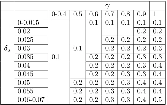
the steady state output level or steady state unemployment. By de…nition, the steady state
levels of output and unemployment are …xed and thus do not depend on past deviations of
unemployment from its steady state. It indeed turns out that if the central bank targets the
steady state, responding to the output gap has a strong stabilising e¤ect. However, the higher
and/ or s; the higher has to be the value of y which guarantees determinacy. Table 5
reports for each combination of and sthe value of y necessary to guarantee determinacy if
2:For = [0;0:4]; y = 0:1guarantees determinacy for the full range of s values. For
= 0:5; y = 0:1 guarantees determinacy for s 0:045; while for s >0:045, determinacy
requires y = 0:2:If the real wage does not respond to changes in an individual worker’s skill
level at all ( = 1), y would have to increase up to 0.5 if s 0:06: Table 6 shows that the
value of y necessary to guarantee determinacy also increases in . It reports the values of
y necessary to guarantee determinacy for 3: For each combination of and s; the
minimum value y required for determinacy is often considerably larger and never smaller
than its value for 2:Targeting the steady state unemployment rate, i.e. replacing(M7)
withbit = Et+j t uubt; j = 0;1 and u = [0; 1]; has a very similar but slightly weaker
e¤ect.19
Hence the introduction of skill decay strengthens the argument made by Blanchard and
Gali (2008) saying that if there is little hiring and …ring, the central bank should focus more
on stabilising unemployment and less on stabilising in‡ation than if the labour market is
very ‡uid. Their optimal simple rule puts a much smaller weight on in‡ation stabilisation
under the European than under the American calibration.20 In the presence of skill decay
19For
u = y =k; withk= [0; 1];the associated upper bound on will frequently be lower by about
0.1-0.3 if the central bank responds to unemployment as compared to when it responds to the deviation of output from its steady state.
and real-wage rigidity, a passive response to in‡ation or a su¢ ciently aggressive response to
unemployment is necessary to rule out multiple equilibria, which clearly is a precondition for
optimality.
5
Dynamics under Indeterminacy
In section 4.2, we suggested that the intuition why a value of s equal to or above the
respective critical level combined with >1induces indeterminacy is as follows: A sunspot
driven persistent decrease in demand and thus increase in unemployment will ultimately
increase marginal cost and in‡ation since <0: If > 1; this will ultimately increase the
real interest rate, thus validating the original increase in unemployment. In this section we
con…rm that this is exactly what happens by investigating the response of the model under
the European calibration to a sunspot shock, with = 0:3 and skill decay s being at the
corresponding critical level of 0.03.
To solve the indeterminate model, we follow a solution method proposed by Lubik and
Schorfheide (2003) who extend an approach by Sims (2002). Lubik and Schorfheide propose to
solve linear rational expectation (RE) models by solving for the vector of expectational errors
et=qt Et 1qt vt, whereqt is a vector of variables over which agents form expectations and
vt is a sunspot shock. If the solution to the model is not unique, vt can trigger self-ful…lling
can be cast into the following form:
0yt= 1yt 1+
2 6 6 4
"t
vt 3 7 7
5+ et (18)
where "t denotes an i.i.d. vector of structural shocks and all variables with a t and t 1
subscript are observable at time t, and all variables with at 1subscript are predetermined.
Lubik and Schorfheide suggest to interpret the vectorvtas belief shocks that trigger reversion
of forecasts of the endogenous variables between t 1 and t.21 We assume that the e¤ects
of the sunspot shock vt and the structural shock "t to the forecast error are orthogonal to
each other. This is a standard assumption in the literature on indeterminate linear rational
expectations models and allows to easily solve the model by casting M1 to M8 in the form
of (18). The vectors yt, "t and vt as well as the matrices 0, 1; and are displayed in
appendix D.
We assume that the central bank responds only to in‡ation and set = 1:5:We consider
the e¤ects of a -2% belief shock to consumption, i.e. vc
0 = 0:02: Figure 3 displays the
deviation of unemployment from its steady state (in percentage points) and consumption (in
percent). Unemployment increases by about 0.9 percentage point, while consumption declines
by a bit less than 0.9% and then declines somewhat further. The increase in unemployment
is very persistent: after ten years, unemployment is still about 0.8 percentage points above
[image:34.612.204.412.106.170.2]its steady state while after 25 years (100 quarters) it still exceeds its steady state by 0.7%.
Figure 4 shows that mcct falls by 0.07% on impact and then starts increasing and turns
positive in quarter 16. Since we have chosen a value of ssuch that is smaller than zero (see
Figure 1, the line for = 0:3), we would expect the persistent increase in unemployment to
ultimately turn marginal cost positive. However, as long as the history of high unemployment
is short, the skill loss among job seekers has not yet su¢ ciently built up to dominate the
hiring cost channel and thus turn marginal cost positive. To illustrate how the dynamic of
the skill decline matches with sign change and dynamic of mcct, note that the skill level
in response to a "permanent" change in the unemployment rate in period t 1 evolves as
b
aLt = au (1 x)t ts 1 u;b whereaudenotes the decrease of the the skill level of the average
applicant caused by a permanent increase in unemployment and is de…ned in proposition 1.
In Figure 5, we plot baL
t (as de…ned in this equation) as a percentage of the change of baL1
after an in…nite number of periods, i.e. 1 (1 x)t ts 100: The curve is rather steep at
the beginning but then ‡attens out. With an unemployment history of 15 quarters, which
happens to be the case in quarter 16, the decline inbaL
t has reached 97.8% of its total and the
rate of change has decreased to about 0.5 percentage points. Thus mcct turns positive after
the decline in the skill level has almost reached its maximum. Note also that the dynamics
of mcct andbaLt are similar in that the rate of increase of mcct is at its highest during those
…rst 15 quarters but then gradually declines.
In‡ation declines to -0.08% on impact but turns positive in quarter four. It then keeps
rising until it reaches a plateau at 0.003% in quarter 19. In‡ation is pushed faster above zero
because it responds not just to current but also to expected future values of marginal costs.
Correspondingly, we would expect the ex ante real interest rate ultimately to increase as well.
Figure 6 shows that (it Et t+1) declines on impact but begins to increase in quarter two and
begins to exceed its steady state value in quarter …ve and then remains persistently above
the initial decline in consumption and the associated increase in unemployment. Hence the
response of consumption, unemployment, marginal cost, in‡ation and the real interest rate
to the sunspot shock is just as we would expect from our discussion in section 4.2.
6
Conclusion
This paper adds duration-dependent skill decay during unemployment as an additional
labour-market friction to the sticky price model with hiring costs and real-wage rigidity
developed by Blanchard and Gali (2008) and shows the implications of this modi…cation for
determinacy. We …nd that, while without skill decay, an active monetary policy ensures
equi-librium uniqueness, this is not true in the presence of skill decay. For a job …nding probability
calibrated at the OECD-European median and very moderate real-wage rigidity, there exists
a critical threshold level of skill decay. If the quarterly skill decay percentage is increased to
or above this level and the central bank responds only to in‡ation, determinacy requires a
coe¢ cient on in‡ation in the interest feedback rule smaller than one. This holds regardless
of whether the central bank responds to current, lagged or expected future in‡ation. The
critical skill decay percentage decreases in the degree of real-wage rigidity and increases in
the job …nding probability. If the job …nding probability is set to a higher "American" value,
no critical value exists within a reasonable range of values for s.
Apparently the switch in the determinacy requirement is related to the e¤ect of skill
decay on the long-run relationship between marginal cost and unemployment. We show
this relationship to be always negative in the absence of skill decay. However, a su¢ cient
the relation and may even turn it positive. The respective critical skill decay percentage
typically equals or is very close to the value of s turning the relationship positive. In such
a world, a persistent increase in unemployment will ultimately increase in‡ation. If the
central bank responds more than one-for-one to in‡ation, the real interest rate increases,
which lowers demand and thus validates the increase in unemployment: Hence we have a
self-ful…lling prophecy. Consistent with this intuition, under the American calibration, the
long-run marginal cost-unemployment relationship never turns positive for reasonable values
of sbecause it is much more negative than under the European calibration due to interaction
of the size of labour market ‡ows under the two calibrations with costly hiring.
The indeterminacy problem under the European calibration can be solved by adding the
output gap to the policy rule if the right target level for output is used. If the central bank
targets the steady state level of output, then a su¢ cient response to the output gap induces
determinacy even if skill decay is above its respective critical level. By contrast, targeting
‡exible price output will increase the indeterminacy region. Adding unemployment to the
policy rule is also stabilising.
Finally, we compute the response of the economy to an adverse consumption sunspot
shock under the European calibration, an active monetary policy and skill decay above its
respective critical level. It turns out that the path of consumption, unemployment, marginal
cost, in‡ation and the real interest rate is in line with our intuition for why an active
mon-etary policy induces indeterminacy under such a parameterization. Further, the response of
References
[1] Addison, J.T./ Portugal, P. (1989), Job Displacement, relative Wage Changes and
Du-ration of Unemployment, in: Journal of Labor Economics, Vol. 7, No. 3, pp. 281-302.
[2] Agell, J./ Lundborg, P. (2003), Survey Evidence on Wage Rigidity and Unemployment:
Sweden in the 1990s, in: Scandinavian Journal of Economics, Vol. 97, pp. 295-307.
[3] Batini, N./ Justiniano, A./ Levine, P./ Pearlman, J. (2006), Robust
In‡ation-forecast-based Rules to shield against Indeterminacy, in: the Journal of Economic Dynamics and
Control, Vol. 30, pp. 1491-1526.
[4] Belke, A./ Klose, J. (2009), Does the ECB rely on a Taylor Rule? Comparing Ex-post
with Real Time Data, DIW Berlin Discussion Paper 917.
[5] Bewley, T. F. (1998), Why not cut Pay?, in: European Economic Review 42, pp. 459-490.
[6] Bewley, T. F. (1999), Why Wages Don’t Fall During a Recession, Harvard University
Press.
[7] Blanchard, O./ Gali, J. (2008), Labor Markets and Monetary Policy: A New-Keynesian
Model with Unemployment, NBER Working Paper 13897, forthcoming in American
Economic Journal - Macroeconomics.
[8] Calvo, G. A. (1983), Staggered Prices in a Utility-Maximising Framework, in: Journal
of Monetary Economics, pp. 983-998.
[9] Carlstrom, C. T./ Fuerst, T. S. (2005), Investment and Interest Rate Policy: a discrete
[10] Christiano, L./ Trabandt, M./ Walentin, K. (2010), DSGE Models for Monetary Policy
Analysis, NBER Working Paper 16074.
[11] Clarida, R./ Gali, J./ Gertler, M. (1998), Monetary Policy rules in practice. Some
in-ternational evidence, in: European Economic Review 42, pp. 1033-1067.
[12] Clarida, R./ Gali, J., Gertler, M. (2000), Monetary Policy Rules and Macroeconomic
Stability: Evidence and some Theory, in: The Quarterly Journal of Economics, Vol.
115, pp. 147-180.
[13] Clausen, J.R./ Meier, C.-P. (2003), Did the Bundesbank follow a Taylor Rule?, IWP
Discussion Paper No 2003/2
[14] Danthine, J.-P./ Kurman, A. (2004), Fair Wages in a New Keynesian model of the
business cycle, in: Review of Economic Dynamics 7, p. 107-142.
[15] Du¤y, J./ Xiao, W. (2008), Investment and Monetary Policy: Learning and Determinacy
of Equilibrium, University of Pittsburgh, Department of Economics Working Papers 324,
http://www.econ.pitt.edu/papers/John_nkk13.pdf
[16] Fabiani, S./ Galuscak, K./ Kwapil, C./ Lamo, A./ Rõõm, T./ Pank, E. (2010), Wage
Rigidities and Labor Market Adjustment in Europe, in: Journal of the European
Eco-nomic Association, Vol. 8(2-3), pp. 497–505.
[17] Falk, A./ Fehr, E. (1999), Wage Rigidity in a Competitive Incomplete Contract Market,
[18] Gali, J. (2001), New Perspectives on Monetary Policy, In‡ation, and the Business
Cy-cle, Prepared for an invited session at the World Congress of the Econometric Society,
Seattle, August 11-16, 2000.
[19] Galušµcák, K./ Keeney, M./ Nicolitsas, D./ Smets, F./ Strzelecki, P./ Vodopivec, M.
(2010), The Determination of Wages of newly hired Employees. Survey Evidence on
internal versus external Factors, ECB Working Paper No. 1153.
[20] Gangji, A./ Plasman, R. (2007), The Matthew E¤ect of Unemployment: How does it
a¤ect Wages in Belgium?, DULBA Working paper No. 07-19.RS.
[21] Gertler, M./ Trigari, A. (2009), Unemployment Fluctuations with Staggered Nash Wage
Bargaining, in: Journal of Political Economy, Vol. 117(1).
[22] Gorter, J./ Jacobs, J./ de Haan, J. (2008), Taylor Rules for the ECB using Expectations
Data, in: Scandinavian Journal of Economics 110(3), pp. 473-488.
[23] Gregg, P./ Tominey, E. (2005), The Wage Scar from male youth Unemployment, in:
Labour Economics, Vol. 12, pp. 487-509.
[24] Gregory, M./ Jukes, R. (2001), Unemployment and Subsequent Earnings : Estimating
Scarring among British Men 1984-94, in: The Economic Journal, Vol. 111, No. 475, pp.
F607-F625.
[25] Hall, R. E. (2005), Employment Fluctuations with Equilibrium Wage Stickiness, in: The
[26] Hobijn, B./ Sahin, A. (2009), Job-…nding and Separation Rates in the OECD, in:
Eco-nomic Letters 104, pp. 107-111.
[27] Kurozumi, T./ Van Zandweghe (2008a), Investment, Interest Rate Policy, and
Equilib-rium Stability, in: Journal of Economic Dynamics and Control 32.
[28] Kurozumi, T./ Van Zandweghe (2008b), Labor Market Search and Interest Rate Policy,
Federal Reserve Bank of Kansas City Working Paper 08-03.
[29] Layard, R./ Nickell, S./ Jackman, R. (1991), Unemployment. Macroeconomic
Perfor-mance and the Labour Market, Oxford University Press.
[30] Levin, A./ Wieland, V./ Williams, J. C. (2003), The Performance of Forecast-based
Monetary Policy Rules Under Model Uncertainty, in: The American Economic Review,
Vol. 93(3), pp. 622-645.
[31] Llosa, L.-G./ Tuesta, V. (2009), Learning about Monetary Policy Rules when the Cost
Channel Matters, forthcoming in: Journal of Economic Dynamics and Control.
[32] Lubik, T.A./ Schorfheide, F. (2003), Computing sunspot equilibria in linear rational
expectations models, in: Journal of Economic Dynamics & Control 28, pp. 273 –285.
[33] Machin, S./ Manning, A. (1999), The causes and consequences of long-term
unemploy-ment in Europe, in: Handbook of Labor Economics, vol. 3, Part C, pp. 3085-3139,
Elsevier.
[34] Mortensen, D. T./ Pissarides, C. A. (1994), Job Creation and Job Destruction in the
[35] Nickell, S./ Jones, P./ Quintini, G. (2002), A Picture of Job Insecurity Facing British
Men, in: The Economic Journal, Vol. 112, No. 476, pp. 1-27.
[36] Orphanides, A. (2001), Monetary Policy Rules based on Real Time Data, in: The
Amer-ican Economic Review, Vol. 91, No. 4, pp. 964-985.
[37] Peersman, G./ Smets, F. (1999), Uncertainty and the Taylor rule in a simple Model of
the Euro-area Economy, in Proceedings, Federal Reserve Bank of San Francisco.
[38] Phelps, E. S. (1972), In‡ation Policy and Unemployment Theory. The Cost-Bene…t
Approach to Monetary Planning, Norton and Company.
[39] Pichelmann, K./ Riedel, M. (1993), Unemployment Duration and the relative Change in
individual Earnings: Evidence from Austrian Panel Data, Research Memorandum No.
317.
[40] Pissarides, C. A. (1992), Loss of Skill During Unemployment and the Persistence of
Employment Shocks, in: The Quarterly Journal of Economics, Vol. 107, No. 4, pp.
1371-1391.
[41] Pissarides, C. A. (2009), The Unemployment Volatility Puzzle: Is Wage Stickiness the
Answer?, in: Econometrica, Vol. 77, pp. 1339-1369.
[42] Rannenberg, A. (2009), The Taylor Principle and (In-) Determinacy in a New Keynesian
Model with hiring Frictions and Skill Loss, CDMA Working Paper 0909.
[43] Ravenna, F., Walsh, C. E. (2006), Optimal monetary Policy with the Cost Channel, in: