MODELLING AND SIMULATION OF SMALL SCALE EMBEDDED GENERATION SYSTEMS
N J Kelly
1, I Beausoleil-Morrison
21
Energy Systems Research Unit, University of Strathclyde, Glasgow, Scotland ([email protected])
2
CANMET Energy Technology Centre, Natural Resources Canada, Ottawa ([email protected])
ABSTRACT
Advances in heat and power production are leading to a revolution in how buildings are perceived as an energy system. The rapid development of fuel cells, photovoltaic facades, cogeneration and the evolution of ducted wind turbines allows the designer to envisage a building providing much of its own heat and power through local embedded generation (EG). However, the addition of heat and power production to the building increases it complexity as an energy system. New design issues must be addressed such as the integration of EG with traditional HVAC and power systems; optimal demand and supply matching; demand side management and its impact on environmental performance; interaction of the EG system with the local electricity network, etc.
Designers have traditionally relied on simulation tools to help answer complex questions relating to building environmental performance. Hence, to assist designers in the development of integrated EG schemes, building simulation tools must evolve to facilitate all aspects of EG systems modelling: EG components, electrical power flow, demand and supply control algorithms, etc. Moreover, to assess the interactions between an EG system and all other components of a building, modelling and simulation must be undertaken in an integrated manner.
This paper describes how the ESP-r simulation tool has been adapted to facilitate the integrated modelling of building EG systems. In particular, the paper looks at:
• the integration of electrical modelling with building and systems simulation; • the development of thermal and electrical
EG component models;
• the development of high level EG system control algorithms;
• integrated modelling of EG systems.
In this paper a solid oxide fuel cell (SOFC) is used as an example of a thermal and electrical component model and to illustrate the integrated thermal and electrical simulation of EG systems the example of a building powered by a fuel cell and PV panels is used. The simulation looks at control of loads and generation sources for optimum supply-demand matching.
INTRODUCTION
The built environment is a major consumer of heat and electricity. The recognition of the environmental damage caused by the wasteful use of this energy coupled with advances in technology has led to a change in the view of the building as an energy system. Technologies such as photovoltaic facades and cogeneration allow a building to produce much of its own heat and power from cleaner sources. This raises new performance-related issues such as the best means of using the supplied heat and power, matching supply with demand, the interaction of the EG components with more traditional plant and suitable control of the EG sources in transient conditions. The answer to most of these questions requires some form of integrated building and systems simulation.
MODELLING OF EMBEDDED GENERATION SYSTEMS
ESP-r is a “multi-domain” model, where a domain is an element of the model describing a building subsystem, the core of which is the building domain, describing the geometry and fabric. This is augmented with one or more technical domains that add functionality and detail, e.g. an HVAC system, airflow, etc. Until recently ESP-r, like most building simulation tools had been targeted at analysis of the thermal performance of buildings, electrical phenomena (lighting control, equipment gains, etc.) being considered only with respect to their affect on thermal conditions. However, in buildings with embedded generation (EG), the production and use of electrical power is strongly coupled to thermal performance, requiring that ESP-r be further developed to facilitate the modelling of electrical systems with the addition of an electrical domain [2]. This domain, like the other ESP-r domains is modelled using a network, comprising a series of nodes, representing control volumes1, connected together to form a system description. The nodes are the points where network state variables (voltage) and derived variables (current, power) are calculated. The connectors between nodes are component models: cables, transformers, inverters, etc. The addition of an electrical network allows the power flow around the building to be tracked as the building simulation evolves over time with climate, occupant interaction and systems control. The network approach can be used to model single phase, multi-phase, d.c. networks and networks comprising a mixture of all three (figure 1).
The solution of the electrical network is based on the application of two power balance equations at each node, which can be expressed as follows:
0 / / / = − + node from drawn power reactive real node at generated power reactive real node from to d transmitte power reactive or real 1
The control volume is an arbitrary region of space to which the laws of conservation of mass, energy and momentum can be applied. Control volumes are the fundamental constituents of all the domains within an ESP-r model.
The power balance at a node i connected to n
other nodes, y generating components and z loads can be expressed mathematically as follows:
0 1 1 ) , cos( 1 , Y = ∑ = ∑ = − + − − ∑ = z
r Lir P y
q Giq P p i p i n
p p i p V i
V θ θ α
(1) 0 1 1 ) , sin( 1 , Y = ∑ = ∑ = − + − − ∑ = z
r Lir Q y
q Giq Q p i p i n
p p i p
V i
V θ θ α
(2)
Equation 1 is the real power balance (W) at each node in the electrical network. This is the power used to do work in power consuming components. Equation 2 is the reactive power balance (VAr) at the same node, this is power used to energise electric or magnetic fields in electrical components. A set of these power balance equations can be extracted from an electrical network and solved iteratively using a Newton-Raphson based solver, modified from that described by Stagg and El-Abiad [3]. During the solution, the complex voltage2, V , at each node, is adjusted until the real and reactive power flows at each node equate to zero. Solution of the electrical network yields:
• the voltage at each point in the network; • current and power flows (real and reactive)
through connecting components; • transmission losses in conductors;
• power imported into the network to maintain stability;
• power factors; • phase loadings;
2
) sin (cosθ j θ V
Figure 1 An example of an electrical network.
The electrical network solution requires that the real and reactive power flows into (generated power) and out of each node (power drawn by loads) are known; these are provided by various component models (lighting, fans, PV, etc.) linked to the electrical network. These components translate between the electrical and thermal domains of the model, converting thermal/ fluid flow phenomena into real and reactive power flow. Examples include photovoltaic components converting solar radiation falling on to the building facade to electrical power, or pumps consuming electrical energy to transport hot water. As these components simultaneously affect the thermal and electrical domains, an integrated approach to the solution is needed.
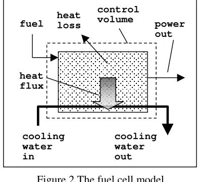
THE FUEL CELL MODEL
A topical example of a linking component is the fuel cell. This technology is generating much interest as a possible source of heat and power for buildings [4,5]. The model described here is based on one created by Beausoleil-Morrison [6]. This component comprised three control volumes but was not developed for linkage into an electrical network. For the purposes of this paper a single control volume (which represents the entire fuel cell), power flow network compatible model has been developed. The component calculates the heat output of the fuel cell based on the electrical loading. Heat to power output characteristics are approximately 0.75:1.
Figure 2 The fuel cell model.
The following equation describes the conservation of energy in the fuel cell control volume.
elec n
j j
fuel q q
t T
Mc = + −
∂ ∂
∑
=1 ϕ
(3)
The term on the left-hand side of the equation represents the heat storage rate in the fuel cell. The three terms on the right hand side of the equation represent the fuel chemical energy flux, the electrical power output and the sum of the other energy fluxes associated with the control volume (heat loss to surroundings, heat transferred to the cooling water, etc.) respectively. Refer to [6] for more details on the fuel cell energy balances. The electrical output of the fuel
fuel
cooling water in
power out
heat flux
heat loss
cooling water out control volume d2 d3
a1 a2 a3
c1 c2 c3
d1 e1 e2 e3
b1 b2 b3
three-phase cable model
f3
g3 h3
i3
single phase section
j1 k1
d.c. section load drawn by coupled
component
power from coupled EG component model electrical
node
inverter model
[image:3.595.326.523.321.501.2]cell can be controlled depending upon the load calculated by the electrical network. Figures 5 and 6 show the fuel cell linked into both an electrical network and an HVAC network. Other examples of ESP-r linking components include lighting, fans and pumps, PV and cogeneration.
EMBEDDED GENERATION SYSTEMS CONTROL
The addition of the electrical network also allows the addition of a new layer of electrical systems control. This is important in embedded generation (EG) systems in that both the supply and demand of power can be controlled to facilitate performance optimisation measures: demand-supply matching, demand reduction, electricity price-based operation, etc.
Control in ESP-r is based on the “control loop” in which a sensor passes information back to a controller (e.g. temperature, flow rate, relative humidity), which then outputs a signal to an actuator (e.g. heat flux, valve, damper, boiler) to change its state and thus attempt to bring a sensed variable (e.g. flow) to a user defined condition. The control loop principle has been extended to the control of electrical systems. ESP-r's range of sensors has been extended to include, voltage, current and power flow sensing. Additional control algorithms have been added specifically for the control of EG systems: demand-supply matching and peak demand limiting.
Control and operation of the EG components and power consuming equipment such as lighting will affect the thermal performance of the building. It is therefore vital that the power system and its control are simulated within the context of an integrated building simulation.
INTEGRATED SOLUTION
ESP-r uses a modular solution process that employs a solution algorithm to control the operation of a number of customised domain solvers (building, HVAC, power flow). The solvers can be thought of as individual blocks that are linked together to form a unified solution process for the model. The solution algorithm determines the structure of the solution process for a particular model, in terms of the solvers used, their interactions and couplings and
temporal relationships. The power flow solver is an integral part of this solver set-up. The solution of the electrical system, together with the other domains of the model enables a simulation to capture the important factors relating to power flow: the switching on and off of power consuming components, control action on lighting, variations in solar radiation on PV, etc.
A typical simulation time step for an integrated model would be 30-120s. The use of this time step means that high frequency transient electrical phenomena are not modelled: the power flow simulation is therefore quasi steady state, each simulation time step solution giving an averaged snapshot of the system operation3.
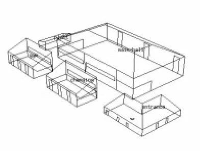
APPLICATION
A small sports centre is shown in figure 4. The building consists of five main areas: a reception, changing rooms, a gym, the main sports hall and a plant room at the rear of the building. Heat and power are provided by a seven 5kW fuel cells integrated into the electrical services and the hot water services (figures 5 and 6). Power is also provided by a 26kW photovoltaic array integrated into the roof of the building model. The loads fed by the hot water services include a heating coil in the HVAC system; this heats the air supplied to the various spaces in the centre, and a hot water calorifier, which links into the domestic hot water services. The hot water flow rates through the calorifier and the heating coil are controlled based on sensed water and hall air temperature respectively. The major electrical loads in the building are the lighting system and the rotational loads (fans and pumps) in the plant system.
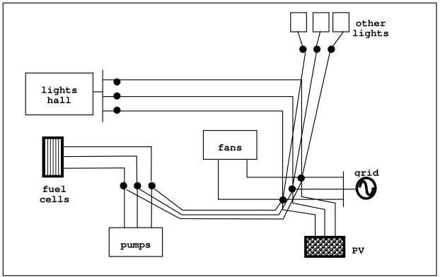
Electrical demand side-management is implemented in that the lighting system is subject to daylight control, affecting both the internal heat gains and electrical demand as ambient lighting conditions change with time. The electrical system of the building is three-phase a.c. and draws power from the fuel cells, PV and a grid connection.
Figure 4 The sports centre model.
Two scenarios for the control of the fuel cell component are simulated: 1) the output of the fuel cells is modulated in an attempt to match the electricity demand of the building; 2) the fuel cell is controlled to operate in peak demand limiting mode so that a maximum demand limit for the building is not exceeded. The simulation is run over the course of a spring week, with the building, plant and electrical networks simulated using a two-minute time step. This time step is sufficient to capture the plant dynamics that affect the operation of the power system.
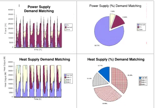
Figure 7 shows some selected output from the demand matching simulation, while figure 8 shows output from the demand limiting simulation.
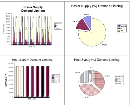
In both figures the power supply graphs show the individual, time-varying contributions from the PV, fuel cells and grid towards meeting the total electrical demand of the building. The power supply pie chart shows the percentage contribution to the total electricity demand from each source over the course of total simulation period (1 week).
The power supply graph of figure 7 clearly shows the modulation of fuel cell output and grid import to accommodate the increased output from the PV. The power supply graph of figure 8 shows that the fuel cells are used only briefly in the morning and in the evening, when the lighting load is high. The fuel cells can be switched off when lighting control reduces the lighting system demand in the middle of the day.
The heat supply graphs of figures 7 and 8 show the individual, time-varying heat output of the fuel cells and three backup boilers. The heat supply pie charts show the percentage contributions to the heating demand from the fuel cells and the backup boilers over the course of the simulation period. Clearly, the fuel cells contribute the most to the heating demand when run under the demand matching control regime.
The information presented here could be further used in and economic analysis of EG system viability.
CONCLUSIONS
This paper has described how the ESP-r simulation tool has been developed to facilitate the modelling of small scale embedded generation through the addition of a electrical domain and new component models: a simple SOFC fuel cell model was presented. The addition of the electrical domain opens up possibilities for the control of EG component models through the calculation of variables such as voltage, current and power flow.
An example application was presented in which the output of the fuel cell model was controlled based on the electrical demand of a sports centre. The total electrical demand (including distribution losses) was calculated using an electrical network. This demand is heavily influenced by control of the lighting system and HVAC system fans and pumps, which in turn are affected by climatic conditions and occupant interaction. Also, as the fuel cell component is an integral part of the HVAC domain, the electrical control also influences the thermal performance of the HVAC system. The thermal performance and electrical performance are therefore closely coupled.
REFERENCES
[1] Clarke J A, Energy simulation in building design (2nd Ed.), Butterworth, Oxford, 2001
[2] Kelly N J, Towards a design environment for building integrated energy systems: the integration of electrical power flow modelling with building simulation, PhD Thesis, University of Strathclyde, Glasgow, 1998.
(ftp://ftp.strath.ac.uk/Esru_public/documents/
kelly_thesis.pdf)
[3] Stagg G and El-Abiad A H, Computer
methods in power systems analysis, McGraw Hill, New York, 1968.
[4] Ellis M.W. and Gunes M.B. 20020, Status of FuelCell Systems for Combined Heat and Power Appli-cations in Buildings, ASHRAE Transactions, AC-02-18-2.
[5] US-DOE (2000), Fuel Cell Handbook, 5th Edition, United States Department of Energy, Morgantown USA.
[6] Beausoleil-Morrison I., Cuthbert D.,Deuchars G., and McAlary G., The simulation of fuel cell
cogeneration systems within residential buildings. Paper to be presented at ESim 2002.
NOMENCLATURE C – specific heat (J/kgK)
M – mass (kg)
P – real power (W)
Q - reactive power (VAr)
q - energy flux (W)
T – temperature (oC)
V – modulus of complex voltage (V)
[image:6.595.138.449.432.628.2]Y±PRGXOXVRIFRPSOH[DGPLWWDQFH -1) – argument of complex admittance (rads) – argument of complex voltage (rads) – fuel chemical potential flux (W)
Figure 5 A fuel cell linked into the electrical network
lights hall
pumps
other lights
fans
fuel cells
Figure 6 A fuel cell linked into the HVAC network.
Figure 7 Thermal and electrical output from the demand matching simulation
Power Supply Demand Matching
Grid
Heat Supply Demand Matching Heat Supply (%) Demand Matching
+
heating coil supply fan
heat exchanger
diverting valves
hot water storage boilers
fuel cells
warm air to building
hot water
[image:7.595.53.547.323.667.2]Figure 8 Thermal and electrical output from the demand limiting simulation