A Novel Nonlinear Evolution Equation Integrable
by the Inverse Scattering Method
Vyacheslav VAKHNENKO † and John PARKES ‡
† Institute for Geophysics, 32 Palladin Ave., Kyiv, 03680, Ukraine
E-mail: [email protected]
‡ Depart. Math., University of Strathclyde, Richmond St., Glasgow G1 1XH, U.K.
E-mail: [email protected]
In this report we consider the nonlinear evolution equation (ut+uux)x+u= 0 (Vakhnenko
equation – VE) that can be integrated by the inverse scattering transform (IST) method. This equation arose as a result describing the high-frequency perturbations in a relaxing medium. The VE has two families of travelling wave solutions, both of which are stable to long wavelength perturbations. In particular, the VE has a loop-like soliton solution. The interaction of two solitons by both Hirota’s method and the IST method are considered. The associated eigenvalue problem has been formulated. This has been achieved by finding a B¨acklund transformation. The inverse scattering method has a third order eigenvalue problem. Under the interaction of solitons there are features that are not typical for the KdV equation.
1
Introduction
Describing real media under the action of intense waves is often unsuccessful in the framework of equilibrium models of continuum mechanics. To develop physical models for wave propagation through media with complicated inner kinetics, the notions based on the relaxational nature of a phenomenon are regarded to be promising. A nonlinear evolution equation is suggested to describe the propagation of waves in a relaxing medium [1]. It is shown that for the low-frequency approach this equation is reduced to the Korteweg-de Vries (KdV) equation. In contrast to the low-frequency perturbations, the high-frequency perturbations satisfy a new nonlinear equation [2]
∂ ∂x
∂ ∂t+u
∂ ∂x
u+u= 0. (1)
The equation (1) has been studied in various Refs. [2, 3, 4, 5, 6, 7, 8, 9]. Hereafter, as was initiated in [3], this equation is referred to as the Vakhnenko equation (VE). There is a certain analogy between the KdV equation and the VE. They have the same hydrodynamic nonlinearity and do not contain dissipative terms; only the dispersive terms are different. It turns out that the VE possesses, at least partially, the remarkable properties inherent to the KdV equation. The study of the VE has scientific interest both from the viewpoint of the existence of stable wave formations and from the viewpoint of the general problem of integrability of nonlinear equations.
2
Physical processes described by the Vakhnenko equation
the propagation of fast perturbations. There are processes of the interaction that tend to return the equilibrium. In essence, the change of macroparameters caused by the changes of inner parameters is a relaxation process.
To analyze the wave motion, we use the hydrodynamic equations in Lagrangian coordinaties:
∂V ∂ t −
1 ρ0
∂ u ∂ x = 0,
∂u ∂ t +
1 ρ0
∂ p
∂ x = 0. (2)
The following dynamic state equation is applied to account for the relaxation effects:
dρ=c−f2dp+τp−1(ρ−ρe)dt. (3)
We note that the mechanisms of the exchange processes are not defined concretely when deriving the dynamic state equation (3). In this equation the thermodynamic and kinetic parameters appear only as sound velocitiesce,cf and relaxation timeτp. These characteristics can be found experimentally.
Let us consider a small nonlinear perturbation p′ < p
0. Combining the relationships (2), (3) we obtain the nonlinear evolution equation in one unknownp (the dash inp′ is omitted) [1]
τp ∂ ∂ t
∂2p ∂ x2 −c
−2
f ∂2p ∂ t2 +αf
∂2p2 ∂ t2
+
∂2p ∂ x2 −c
−2
e ∂2p ∂ t2 +αe
∂2p2 ∂ t2
= 0. (4)
A similar equation has been obtained by Clarke [10], but without nonlinear terms.
In [1] it is shown that for low-frequency perturbations (τpω≪1) the equation (4) is reduced to the Korteweg-de Vries – Burgers (KdVB) equation
∂ p ∂ t +ce
∂ p ∂ x +αec
3
ep ∂ p ∂ x −βe
∂2p ∂ x2 +γe
∂3p ∂ x3 = 0,
while for high-frequency waves (τpω ≫1) we have obtained the new equation
∂2p ∂ x2 −c
−2
f ∂2p ∂ t2 +αfc
2
f ∂2p2
∂ x2 +βf ∂ p
∂ x +γfp= 0. (5)
The nonlinear equation (5) has dissipativeβf∂ p/∂ xand dispersiveγfpterms. Without nonlinear and dissipative terms, we have a linear Klein–Gordon equation.
In the general case the last equation has been investigated insufficiently. It is likely that this is connected with the fact, noted by Whitham [11], that the high-frequency perturbations attenuate very fast. However in Whitham’s monograph, the evolution equation without nonlinear and dispersive terms was considered. Certainly, the lack of such terms restricts the class of solutions. At least, there is no solution in the form of a solitary wave, which is caused by nonlinearity and dispersion.
3
Evolution equation for high-frequency perturbations
The equation (5), which we are interested in, is written down in dimensionless form. In the moving coordinates system with velocitycf, the equation has the form in dimensionless variables
˜ x=
γf
2 (x−cft), ˜t=
γf
2cft, ˜u=αfc2fp(tilde over variables ˜x, ˜t, ˜u is omitted)
∂ ∂x
∂ ∂t+u
∂ ∂x
u+α∂u
The constant α =βf/
2γf is always positive. Equation (6) without the dissipative term has the form of the nonlinear equation [2, 3] (see equation (1))
∂ ∂x
∂ ∂t+u
∂ ∂x
u+u= 0. (7)
The travelling-wave solutions of the VE (7) were derived in [2, 3], and its symmetry properties were studied in [5]. A remarkable feature of the VE is that it has a soliton solution which has loop-like form, i.e. it is a multi-valued function (see Fig. 1 in [2]). Whilst loop soliton solutions are rather intriguing, it is the solution to the initial value problem that is of more interest in a physical context.
The physical interpretation of the multi-valued functions that describe the loop-like soliton solutions was given in [1]. The problem is whether the ambiguity has a physical nature or is related to the incompleteness of the mathematical model, in particular to the lack of dissipation. It is significant that the loop-like solutions are stable to long-wavelength perturbations [3], and that the introduction of a dissipative term (see equation (6)), with dissipation parameter less than some limiting value, does not destroy these loop-like solutions [1]. Since the solution has a parametric form [2, 3], there is a space of variables in which the solution is a single-value function. Consequently, the ambiguity of solution does not relate to the incompleteness of the mathematical model. Thus in the framework of this model approach, the high-frequency perturbation can be described by the multi-valued functions [1].
We have succeeded in finding new coordinates (X, T), in terms of which the solution of equation (1) is given by single-valued parametric relations. New independent coordinates X,T are defined as [4]
x=x0+T+W(X, T), t=X, W =
X
−∞
U(X′, T)dX′. (8)
Hereu(x, t) =U(X, T), andx0is a constant. We also assume that, asX → −∞, the derivatives of W vanish andW tends to a constant. Equation (1) then has the form [4, 8]
WXXT + (1 +WT)WX = 0. (9)
If the solutionU(X, T) =WX of the transformed VE (9) has been obtained, the original inde-pendent space coordinatexcan be found by means of the formula (8). This relationship together with u(x, t) =U(X, T) enables us to define the solution of the VE in parametric form withT as parameter. We note that the transformation (9) between old and new coordinates is similar to the transformation between Eulerian variables (x, t) and Lagrangian variables (T, X) [8].
Finally, by taking W = 6(lnf)X, where f is a function of X and T, we observe that the transformed VE (9) may be written as the bilinear equation [4]
DTDX3 +DX2
f ·f = 0, (10)
whereD is the Hirota binary operator [12].
4
B¨
acklund transformation for the transformed
Vakhnenko equation
soliton problems and has a close relationship to the IST method [12, 13, 14]. First we define P as follows:
P :=
DTDX3 +DX2
f′·f′ f f−f′f′
DTDX3 +D2X
f ·f .
We aim to find a pair of equations such that each equation is linear in each of the dependent variables f and f′, and such that togetherf and f′ satisfyP = 0. The pair of equations is the
required B¨acklund transformation.
Combining this relationship we can rewriteP in the following form [8]:
P = 2DT
D3X−λ(X)
f′·f
·(f′f)−2DX({3DTDX+ 1 +µ(T)DX}f′·f)·(DXf′·f). Thus we have proved [8] that the B¨acklund transformation is given by the two equations
D3X −λ
f′·f = 0, (11)
(3DXDT + 1 +µDX)f′·f = 0, (12)
where λ=λ(X) is an arbitrary function of X and µ=µ(T) is an arbitrary function of T. In original form withµ= 0 we have
(W′−W) XX+
1 2(W
′−W)(W′+W) X +
1 36(W
′−W)3−6λ= 0, (13)
(W′−W)
3(W′+W)XT + 1 2(W
′
−W)(W′−W)T
−6(W′−W)X
1 +1 2(W
′+W) T
= 0. (14)
Separately the two equations (11), (12) appear as part of the B¨acklund transformation for other nonlinear evolution equations. For example, equation (11) is the same as one of the equations that is part of the B¨acklund transformation for a higher order KdV equation (see equation (5.139) in [12]), and equation (12) is similar to (5.132) in [12] that is part of the B¨acklund transformation for a model equation for shallow water waves [15].
5
Interaction of the solitons
The transformation into new coordinates (8) is the key to solving the problem of the interaction of the solitons. The exactN-soliton solutions are obtained by use of (i) Hirota’s method [4, 7]; (ii) elements of the inverse scattering transform procedure for the KdV equation (spectral equa-tion of second order – Schr¨odinger equation) [6]; (iii) the inverse scattering transform procedure (spectral equation of third order) [9].
Since the equation (1) can be written in bilinear form (10), Hirota’s method enables us to find soliton solutions. These solutions have been obtained in [4, 7], for example, for the one-soliton solution
f = 1 + exp (2η), W = 6(lnf)X, η =kX−ωT +α, U =WX = 6k2sech2η,
and for the two-soliton solution
f = 1 + exp (2η1) + exp (2η2) +b2exp (2η1+ 2η2), W = 6(lnf)X,
b2 = F[2 (k1−k2),−2 (ω1−ω2)] F[2 (k1+k2),−2 (ω1+ω2)]
= (k2−k1) 2
(k2+k1)2 k2
1 +k22−k1k2 k2
1 +k22+k1k2 ,
Now we present IST method for finding the solution of the VE. The IST is the most appro-priate way of tackling the initial value problem. The results of applying the IST method would be useful in solving the Cauchy problem for the VE. In order to use the IST method one first has to formulate the associated eigenvalue problem.
Introducing the functionψ=f′/f, we find that equations (11), (12) reduce to
ψXXX+U ψX −λψ = 0, (15)
3ψXT + (WT + 1)ψ+µψX = 0, (16)
respectively. It may be shown
[WXXT + (1 +WT)WX]Xψ+λX(3ψT +µψ) = 0.
Hence equation (9) is the condition for λX = 0, and hence for λ to be constant. Constant λ (spectral parameter) is what is required in the IST problem.
Thus the IST problem is directly related to a spectral equation of third order (15). The third order eigenvalue problem is similar to the one associated with a higher order KdV equation [16, 17], a Boussinesq equation [16, 18], and a model equation for shallow water waves [12, 19].
Kaup [16], Caudrey [18, 20] and Deift et al. [21] studied the inverse problem for certain third order spectral equations. We adapt the results obtained by these authors to the present problem and describe a procedure for using the IST to find the N-soliton solution to the transformed VE, and hence to the VE itself.
We proved that theT-evolution of the scattering data is given by the relationships [9] (k= 1,2, . . . ,2N)
ζj(k)(T) =ζj(k)(0),
γ1(kj)(T) =γ1(kj)(0) exp
−3λj
ζ1(k)−1+3λ1
ζ1(k)−1
T
. (17)
Here λj(ζ) =ωjζ,λ3j(ζ) =λ, and ωj =ei2π(j−1)/3 are the cube of roots of 1.
The final result for the N-soliton solution of the transformed VE is given by the relation [9]
U(X, T) = 3 ∂ 2
∂X2ln (detM(X, T)), (18)
whereM is the 2N×2N matrix given by
Mkl=δkl−
3
j=2
γ1(kj)(0) exp
−3λj
ζ1(k)−1+3λ1
ζ1(k)−1
T+λj
ζ1(k)−λ1
ζ1(l)X
λj
ζ1(k)−λ1
ζ1(l)
, (19)
and the scattering data is calculated from constants ξm,βm as
n= 1, 2, . . . , N, m= 2n−1, λ1
ζ1(m)= iω2ξm, λ2
ζ1(m)= iω3ξm, γ12(m)(0) =ω2βm, γ(13m)(0) = 0,
λ1
ζ1(m+1)=−iω3ξm, λ3
ζ1(m+1)=−iω2ξm, γ12(m+1)(0) = 0, γ (m+1)
13 (0) =ω3βm.
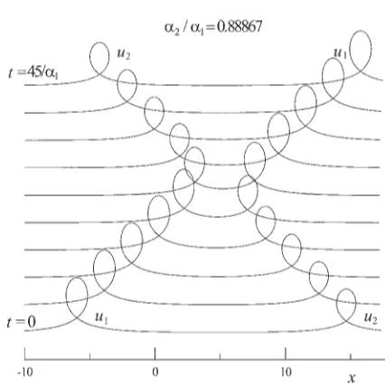
Figure 1. Interaction of two solitons in moving coordinates at time interval ∆t= 70/α1.
Figure 2. The phaseshifts of the smaller soliton is zero. Time interval is ∆t= 5/α1.
For example, the matrix for one-soliton solution has a form
1−√ω2β1 3ξ1
exp√3ξ1X−(
√
3ξ1)−1T
iω3β1
2ξ1
exp2iω3ξ1X−(
√
3ξ1)−1T
−iω2β1 2ξ1
exp−2iω2ξ1X−(
√
3ξ1)−1T
1−√ω3β1
3ξ1
exp√3ξ1X−(
√
3ξ1)−1T
. (20)
Calculating the determinant
detM =
1 + β1 2√3ξ1
exp
√
3ξ1
X− T
3ξ2 1
2
,
we have from (18) the one-soliton solution of the transformed VE as obtained by the IST method
U = 3 ∂ 2
∂X2 ln (detM(X, T)) = 9 2ξ
2 1sech2
√
3 2 ξ1
X− T
3ξ2 1
+α1
, (21)
whereα1= 12ln(β1/2√3ξ1) is an arbitrary constant.
The determinant of the matrix for two-soliton solution has a form
detM =
1 +q21+q22+b2q12q222
, (22)
where
qi = exp √
3 2 ξi
X− T
3ξ2
i
+αi
, b2 =
ξ2−ξ1 ξ2+ξ1
2
ξ12+ξ22−ξ1ξ2 ξ2
1+ξ22+ξ1ξ2 ,
and αi = 12ln(βi/2√3ξi) are arbitrary constants.
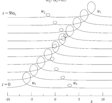
[image:6.595.79.284.101.290.2]Figure 3. Both solitons have phaseshifts in the same direction. Time interval is ∆t= 1/α1.
After the nonlinear interaction the solitons separate, their forms are restored, but phaseshifts arise. The larger soliton always has a forward phaseshift, while the smaller soliton can have three kinds of phaseshift. Note that this property is not typical for the KdV equation. There is a special value of the ratio (α2/α1)∗ = 0.88867. The different kinds of phaseshift are illustrated in Figs. 1–3.
• Forα2/α1 >(α2/α1)∗ the phaseshift of smaller soliton is in the opposite direction to the phaseshift of the larger soliton (Fig. 1).
• Forα2/α1 = (α2/α1)∗ the smaller soliton has no phaseshift (Fig. 2).
• Forα2/α1<(α2/α1)∗less critical value both solitons have phaseshifts in the same direction (Fig. 3).
Acknowledgements
This research was supported in part by STCU, Project N 1747.
[1] Vakhnenko V.O., High-frequency soliton-like waves in a relaxing medium,J. Math. Phys., 1999, V.40, 2011– 2020.
[2] Vakhnenko V.A., Solitons in a nonlinear model medium,J. Phys. A: Math. Gen., 1992, V.25, 4181–4187.
[3] Parkes E.J., The stability of solutions of Vakhnenko’s equation,J. Phys. A: Math. Gen., 1993, V.26, 6469– 6475.
[4] Vakhnenko V.O. and Parkes E.J., The two loop soliton solution of the Vakhnenko equation,Nonlinearity, 1998, V.11, 1457–1466.
[5] Boyko V.M., The symmetrical properties of some equations of the hydrodynamic type, in Proceedings Institute of Mathematics of NAS of Ukraine “Symmetry and Analitic Methods in Mathematical Physics”, 1998, V.19, 32–37.
[6] Vakhnenko V.O., Parkes E.J. and Michtchenko A.V., The Vakhnenko equation from the viewpoint of the inverse scattering method for the KdV equation,Inter. J. Dif. Eq. Appl., 2000, V.1, 429–449.
[7] Morrison A.J., Parkes E.J. and Vakhnenko V.O., TheN loop soliton solution of the Vakhnenko equation, Nonlinearity, 1999, V.12, 1427–1437.
[9] Vakhnenko V.O. and Parkes E.J., A novel nonlinear evolution equation integrable by the inverse scattering method,Rep. NAS Ukr., 2001, N 7, 81–86.
[10] Clarke J.F., Lectures on plane waves in reacting gases,Ann. Phys. Fr., 1984, V.9, 1–211.
[11] Whitham G.B., Linear and nonlinear waves, New York, Wiley-Interscience, 1974.
[12] Hirota R., Direct methods in soliton theory, in Solitons, Editors R.K. Bullough and P.J. Caudrey, New York, Springer, 1980, 157–176.
[13] Hirota R., A new form of B¨acklund transformationand its relation to the inverse scattering problem,Progr. Theor. Phys., 1974, V.52, 1498–1512.
[14] Miura R.M. (Editor), B¨acklund transformations, the inverse scattering method, solitons, and their applica-tions, New York, Springer-Verlag, 1976.
[15] Hirota R. and Satsuma J., N-soliton solutions of model equations for shallow water waves, J. Phys. Soc. Japan, 1976, V.40, 611–612.
[16] Kaup D.J., On the inverse scattering problem for cubic eigenvalue problems of the classψxxx+6Qψx+6Rψ=
λψ,Stud. Appl. Math., 1980, V.62, 189–216.
[17] Satsuma J. and Kaup D.J., A B¨acklund transformation for a higher order Korteweg-de Vries equation, J. Phys. Soc. Japan, 1977, V.43, 692–697.
[18] Caudrey P.J., The inverse problem for a generalN×N spectral equation,Physica D, 1982, V.6, 51–66.
[19] Hirota R. and Satsuma J., A variety of nonlinear network equations generated from the B¨acklund transfor-mation for the Toda lattice,Suppl. Progr. Theor. Phys., 1976, N 59, 64-100.
[20] Caudrey P.J., The inverse problem for the third order equation uxxx+q(x)ux+r(x)u = −iζ3u, Phys.
Lett. A, 1980, V.79, 264–268.