Habitat and host factors associated with liver fluke (Fasciola hepatica) diagnoses in wild red deer (Cervus elaphus) in the Scottish Highlands

RESEARCH

Habitat and host factors associated with liver

fluke (

Fasciola hepatica

) diagnoses in wild red

deer (

Cervus elaphus

) in the Scottish Highlands

Andrew S. French

_{, Ruth N. Zadoks}

_{, Philip J. Skuce}

_{, Gillian Mitchell}

_{, Danielle K. Gordon‑Gibbs}

and Mark A. Taggart

Abstract

Background: Red deer (Cervus elaphus) are a common wild definitive host for liver fluke (Fasciola hepatica) that have been the subject of limited diagnostic surveillance. This study aimed to explore the extent to which coprological diagnoses for F. hepatica in red deer in the Scottish Highlands, Scotland, are associated with variability among hosts and habitats.

Methods: Our analyses were based on coproantigen ELISA diagnoses derived from faecal samples that were col‑ lected from carcasses of culled deer on nine hunting estates during two sampling seasons. Sampling locations were used as centroids about which circular home ranges were quantified. Data were stratified by season, and associa‑ tions between host, hydrological, land cover and meteorological variables and binary diagnoses during 2013–2014 (n= 390) were explored by mixed effect logistic regression. The ability of our model to predict diagnoses relative to that which would be expected by chance was quantified, and data collected during 2012–2013 (n= 289) were used to assess model transferability.

Results: During 2013–2014, habitat and host characteristics explained 28% of variation in diagnoses, whereby half of the explained variation was attributed to differences among estates. The probability of a positive diagnosis was positively associated with the length of streams in the immediate surroundings of each sampling location, but no non‑zero relationships were found for land cover or lifetime average weather variables. Regardless of habitat, the probability of a positive diagnosis remained greatest for males, although males were always sampled earlier in the year than females. A slight decrease in prediction efficacy occurred when our model was used to predict diagnoses for out‑of‑sample data.

Conclusions: We are cautious to extrapolate our findings geographically, owing to a large proportion of variation attributable to overarching differences among estates. Nevertheless, the temporal transferability of our model is encouraging. While we did not identify any non‑zero relationship between meteorological variables and probability of diagnosis, we attribute this (in part) to limitations of interpolated meteorological data. Further study into non‑inde‑ pendent diagnoses within estates and differences among estates in terms of deer management, would improve our understanding of F. hepatica prevalence in wild deer.

Keywords: Wildlife disease, Cervidae, Coproantigen ELISA, Geographical information system, Infection risk factors

© The Author(s) 2019. This article is distributed under the terms of the Creative Commons Attribution 4.0 International License (http://creat iveco mmons .org/licen ses/by/4.0/), which permits unrestricted use, distribution, and reproduction in any medium, provided you give appropriate credit to the original author(s) and the source, provide a link to the Creative Commons license, and indicate if changes were made. The Creative Commons Public Domain Dedication waiver (http://creativecommons.org/ publicdomain/zero/1.0/) applies to the data made available in this article, unless otherwise stated.

Open Access

*Correspondence: Andrew.French@Marine.ie

Background

Liver fluke (Fasciola hepatica) risk to grazing rumi-nants in Europe increased during the 1990s [1] and was reflected in Great Britain (GB) by an increase in the diag-nostic rates of liver fluke in sheep and cattle [2, 3]. During the same period, F. hepatica occurrence in common wild definitive hosts, such as cervids, received only fleeting attention, e.g. as part of histopathological surveys of red (Cervus elaphus) and sika (Cervus nippon) deer in Scot-land [4].

Fasciola hepatica has long-recognised detrimental effects on health and productivity of sheep and cattle [5,

6], and a similar effect might be hypothesised for wild herbivores. More recently, a link between F. hepatica infection, decreased immune response and increased risk of infection of cattle by verocytotoxin producing Escheri-chia coli 0157 has been proposed [7, 8]. In light of pos-sible links such as this, coupled with (for example) an outbreak of E. coli 0157 in autumn 2015 linked to wild sourced venison [9], identification of environments in which wild deer might acquire F. hepatica infection is of interest.

The persistence of F. hepatica in a definitive host popu-lation is dependent on sufficient moisture and warmth (> 10  °C) to facilitate F. hepatica egg development, the motility of free-living larval stages and the activity of a locally resident intermediate host, e.g. Galba truncatula [10, 11]. Where definitive and intermediate hosts are resident in a temperate climate, e.g. in a large propor-tion of GB (England and Wales), the summer risk of F. hepatica infection is predictable based on the principle that transmission is limited primarily by moisture during the summer months (i.e. the balance between rainfall and evapotranspiration; [12]). However, the extent to which this principle is valid for comparatively drier/wetter or warmer/cooler climates, or for animals where infection of the host is not interrupted by anthelminthic treat-ment, is unclear. For example, drier regions can experi-ence a negative correlation between F. hepatica incidence and rainfall (e.g. in Belgium; [13]), owing to an increase in fresh vegetation growth away from permanent water sources around (and in) which intermediate hosts reside.

Red deer in the Scottish Highlands are exposed to a prevailing wet (extreme in GB context) climate with regional averages of 1700 mm of rainfall and 207 days of rain per year (1981–2010 climate period; [14]). This is in excess of the limitations proposed by Ollerenshaw [15], beyond which the relationship between weather and incidence ceases to be valid. Fasciola hepatica preva-lence in red deer varies temporally [16] and geographi-cally throughout the Highlands [17]. While geographical variation could be related to F. hepatica development in certain areas of the Scottish Highlands being limited by

temperature [18], the landscape is markedly different from the pasture dominated rural areas of England and Wales in which temperature-moisture relationships were originally validated. As such, the Scottish Highlands are topographically diverse and offer a range of microcli-mates and a patchwork of habitats (dominated by heather and blanket bog) that might or might not provide tolera-ble environments for intermediate hosts, including atypi-cal hosts such as Radix balthica [19].

The aim of this study was to use coproantigen ELISA (cELISA) surveillance data from wild red deer faecal sam-ples to explore spatial variation in F. hepatica diagnoses in the Scottish Highlands in relation to a suite of host, hydrological, meteorological and land cover variables at the individual level. In so doing, we aim to identify fac-tors associated with F. hepatica diagnosis in wild red deer.

Methods

units; EU) of a positive control antigen supplied with the kit. For frozen faeces, the sensitivity of the cELISA to patent infection (using faecal egg identification to define 52 known positives) was 79% (95% CI: 73–84%) and for fresh faeces (using faecal egg identification to define 18 known positives) it was 50% (95% CI: 32–78%). The specificity of the cELISA to patent infection (using liver examination to define 47 known negatives) was 96% (95% CI: 95–100%), whereby all faeces were fresh.

In the interests of balancing our statistical analysis, data for calves and yearlings were removed from the dataset prior to analyses as not all estates had sampled calves and yearlings for both sampling seasons, whereas data for young, mature and old deer were retained and were con-sidered representative of a single class of “independent deer” (n= 679; see Table 1 for breakdown of sample sizes related to sex and each sampling season).

Geographical information systems and explanatory variable (covariate) preparation

Daily mean temperature (°C) and rainfall (mm) data were obtained for the period 1960–2013 from the UK Meteorological Office’s interpolated 5 km square grid cell dataset [20]. Owing to the disparity between the

downloaded from the UK government website [28] and converted to raster format using Quantum GIS v2.18.2 [29].

Covariate data relating to the immediate surround-ings of each cull location, i.e. 2 km home range radii (12.6 km2_{) buffers created using the gBuffer() function in} the rgeos R package [30] were paired with sample diag-noses using R. Home ranges for individuals that had been culled within 2 km of the coast were clipped to the coastline and were delineated as (relatively) smaller home ranges. Hydrological data were extracted using the st_ intersection() function in the sf R package [31], and land cover and meteorological data were extracted using the extract() function in the raster R package [32]. All spatial data were plotted in R using the rgdal and PBSmapping R packages [33, 34]. Three land cover covariates (smooth grassland, heather moor and blanket bog), which were present in delineated home ranges on all nine estates dur-ing both sampldur-ing seasons for both sexes, were quantified as the proportion of home range area occupied by each cover type (Fig. 2). One hydrological covariate (stream length) was quantified as the total length of streams within each home range. Two meteorological covariates

(rainfall total and development days) were quantified as the mean annual rainfall and mean annual development days experienced across approximate deer lifetimes (i.e. 5 years: 2008–2012 for deer culled during 2012–2013, and 2009–2013 for deer culled during 2013–2014).

Statistical analyses

All statistical analyses were carried out using R 3.5.2 and RStudio v1.1.383 [21, 35] and we followed Zuur & Ieno’s [36] protocol for conducting and presenting regression type analyses and the worked example of a generalised linear mixed effect model of Elston et al. [37].

Owing to marked environmental gradients in rainfall [38] that inhibited spatially blocked cross-validation [39], we stratified our data by sampling season to obtain a data-set for model training and validation (n(2013–2014) = 390; 96 positive cELISA diagnoses, 62 male, 34 female; 294 negative cELISA diagnoses, 149 male, 145 female) and a test dataset to assess the transferability of relationships quantified for the training data (n(2012–2013) = 289; 76 posi-tive cELISA diagnoses, 57 male, 19 female; 213 negaposi-tive cELISA diagnoses, 116 male, 97 female) (i.e. model trans-ferability to an independent dataset; [40]).

Table 1 Sample sizes and Fasciola hepatica coproantigen ELISA diagnoses for red deer (Cervus elaphus) faecal samples collected from nine hunting estates in the Scottish Highlands during two sampling seasons (2012–2013 and 2013–2014)

Abbreviations: F, female deer; M, male deer; NaN, not a number

Key: +, positive cELISA diagnoses; -, negative cELISA diagnoses

Estate Sex 2012–2013 2013–2014

n − + Prevalence n − + Prevalence

Alladale F 23 20 3 13.0 29 27 2 6.9

M 32 25 7 21.9 37 32 5 13.5

Altnaharra F 29 19 10 34.5 29 25 4 13.8

M 31 17 14 45.2 28 12 16 57.1

Applecross F 8 7 1 12.5 16 13 3 18.8

M 32 17 15 46.9 26 12 14 53.8

Ardnamurchan F 5 5 0 0 10 8 2 20.0

M 16 10 6 37.5 25 20 5 20.0

Badanloch F 21 21 0 0 34 33 1 2.9

M 25 21 4 16.0 27 23 4 14.8

Ben Loyal F 22 20 2 9.1 16 14 2 12.5

M 16 12 4 25.0 24 22 2 8.3

Conaglen F 7 4 3 42.9 17 11 6 35.3

M 13 10 3 23.1 17 12 5 29.4

North Harris and Aline F 0 0 0 NaN 11 2 9 81.8

M 6 3 3 50.0 2 2 0 0

Strathconon F 1 1 0 0 17 12 5 29.4

M 2 1 1 50.0 25 14 11 44.0

All F 116 97 19 16.4 179 145 34 19.0

M 173 116 57 32.9 211 149 62 29.4

Owing to the Bernoulli distribution of our diagnostic response data and the nested structure of our sampling design, we implemented a binomial (logistic) generalised linear mixed effect model (GLMM) using the glmer() function in the lme4 R package [41]. Here, we assumed that conditional on random intercept, Estatei, and eight

covariates, the presence-absence data, Yij (jth

obser-vation on estate i), were binomially distributed with a

conditional probability pij, whereby the response Yij was

1 if faecal sample j on estate i was diagnosed positive and was 0 otherwise (Equation 1). The relationship between pij and the linear predictor was determined by the logit

link function, and the random intercept Estatei=1, … , 9

was assumed to be normally distributed with mean 0 and variance σEstate (Equation 2 1).

Fig. 2 Land cover types on nine hunting estates in the Scottish Highlands. The scale‑bar at the top left of each map represents a 4 × 1 km2 _area.

Prior to modelling, each continuous fixed effect covari-ate was mean-centred and scaled to standard deviation units using the scale() function in R, and collinearity between fixed effect covariates were assessed by Pear-son’s R and point-biserial correlations using the chart. Correlation() function in the PerformanceAnalytics R package [42]. We acknowledged prior to modelling that collinearity would be inherent between sex and sam-pling date, because the males and females were sampled during separate Scottish hunting seasons. This collin-earity was a cause for concern for two reasons. First, we would expect inflated variances for sex and sampling date model coefficient estimates. Secondly, we could not be sure whether any observed non-zero associations that each of these variables might have with F. hepatica diag-nostic probabilities (for our dataset) would reflect true underlying associations in nature had samples for both sexes been collected concurrently. Nevertheless, sex (as a binary variable defined as: males = 1 and females = 0) and sampling date were included in our model owing to their assumed meaningful associations with infec-tion, both in terms of red deer feeding behaviour (i.e. chance of encountering F. hepatica metacercariae) and F. hepatica’s life-cycle (i.e. seasonal infection/development and detectability of excretory-secretory antigens within definitive host faeces).

To validate our model, we used the DHARMa R pack-age [43] to simulate scaled (standardised) model residu-als using the simulateResiduresidu-als() function, which we then visually inspected versus fitted values, versus each fixed effect covariate, versus time and in space. Our model was deemed valid if standardised residuals were uniformly distributed showing no trends versus fitted values, and if plotting residuals against time and in two-dimensional space revealed no clear trends or clusters, respectively.

We assessed model prediction efficacy using block cross-validation [39]. Here, we used the roc() and auc() functions in the pROC R package [44] to calculate the area under the receiver operating characteristic curve (AUC). Using the AUC, we inferred the model’s ability to correctly assign high probabilities to positive cELISA diagnoses and low probabilities to negative diagnoses for the training and testing datasets. Here, we used the definitions provided by Swets [45] to define models of low accuracy (AUC 0.50–0.70) and useful accuracy (AUC

(1)

Yij ∼Bin

1,pij

E

Yij=pij

logit

pij

=α+β1×sexij+β2×DateCulledij+β3

×StreamLengthij+β4×BlanketBogij+β5

×HeatherMoorij+β6×SmoothGrasslandij+β7

×RainfallTotalij+β8×DevelopmentDaysij+Estatei

Estate∼_N

0,σ_Estate2

0.70–0.90). We also applied Swets’ [45] interpretation that the AUC corresponds to the percentage of the time that, for a given randomly selected positive and a ran-domly selected negative diagnosis, our model predicts a higher probability for the positively diagnosed sample (bearing in mind that an AUC of 0.50 would be calculated for a model that is no better than would be expected by chance). We also estimated the sensitivity and specific-ity of the model, whereby we used a predicted probabilspecific-ity threshold of 0.50 to signify positive predictions.

Consistent with the logistic and random intercept form of our model, we estimated effective sample size, Neff, (Equation 2), and with it, our model’s inclination towards over parameterization and therefore overfitting [46]. This calculation required: (i) an estimate of random intercept variance, σEstate , to calculate the (induced) intra-class 2 correlation coefficient, ICC [47] (i.e. a quantification of non-independence of events within sampling estates, or “compound symmetry”; Equation 3); (ii) the number of random effect levels in our training data, N, (here, N = 9 estates); and (iii) the number of events per estate, n (here, n = 10.7; i.e. assuming 96 positive diagnoses are spread evenly across all nine estates). In advance of model fit-ting, we calculated an ICC of no greater than 0.021 would correspond with a large enough effective sample size to satisfy the recommended minimum of ten events per variable that would mitigate risk of overfitting a logistic regression type model [48]. Following model training, we used the icc() function in the sjstats R package [49] to corroborate our ICC (as calculated using Equation 3). While our modelling approach ensured that parameter estimates provided by glmer() in lme4 defaulted to Laplace approximation and thus provided a point esti-mate of σEstate , we obtained a 95% confidence interval 2 for σEstate by using the confint.merMod() method in the 2 lme4 R package [41], whereby we used profile intervals to propagate uncertainty for the ICC. Note that increasing quadrature points using glmer(nAGQ = 50) did not change model coefficient estimates.

To help us to evaluate model transferability (i.e. to give context to any differences between the prediction efficacy of the model that occurred between training (2013–2014) and test (2012–2013) data), we estimated the influence of data on model parameter estimates attributable to each individual observation and to observations grouped by (2) Neff =

(N×_n) (1+(n−1)ICC)

(3)

ICC = σ

2

Estate

σ_Estate2 +

π2 3

estate. Here, we used the influence() and cooks.distance() functions in the influence.ME R package [50] to calcu-late the Cook’s distance summary statistic. The strongest influence attributable to data related to individual obser-vations or random effect levels was identified by the largest Cook’s distances.

The variability in the data captured by our model was estimated using marginal and conditional R2 _{[51] using} the rsquared() function in the piecewiseSEM R package [52]. With the exception of the categorical variable, sex (for which an odds ratio was calculated by exponentiating its model coefficient estimate), strengths and directions of relationships between fixed effect covariates and prob-ability of F. hepatica diagnosis (i.e. effect sizes) were inferred from the magnitudes and directions of model parameter estimates. Moreover, non-zero relationships between diagnostic probabilities and each fixed effect covariate

xk=1,...,8

(estimated using the “profile” confint. merMod() method in the lme4 R package [41]) and their respective 95% confidence intervals for each sex were illustrated using logistic regression (Equation 4) and an adapted version of the logi.hist.plot function in the pop-bio R package [53].

Results

Descriptive analysis of spatial aggregation in F. hepatica

diagnosis

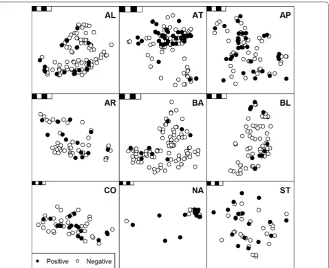
Positive F. hepatica cELISA diagnoses generally displayed a random spatial distribution relative to negative diagno-ses (Fig. 3).

Fasciola hepatica diagnosis in relation to habitat and host variation

Data exploration and model validation

A full list of explanatory variables and their ranges for males and females for each sampling season is presented in Table 2. Only one correlation between two fixed effect covariates exceeded the |R| > 0.70 stipulated by Dormann et al. [54] as a warning as to when multicollinearity might affect the stability of regression parameter estimates; unsurprisingly, this was the point-biserial correlation (|R| = 0.81; 95% CI: 0.77–0.84) between sex and cull date.

Model validation revealed no strong non-linearity (Additional file 1: Figure S1), residual temporal auto-correlation (Additional file 2: Figure S2), nor residual spatial autocorrelation (Moran’s I: Expected = −0.0026, Observed = 0.041, P = 0.22) (Additional file 3: Figure S3). Our assumption of linear relationships between model covariates and the logit link transformed expectation of (4) p= eα+βk xk±1.96(σEstate)

1+_eα+βk xk±1.96(σEstate)

the response were validated by residual plots, though we noted a possible borderline non-linear relationship for smooth grassland (Additional file 1: Figure S1).

Model parameter estimates, prediction efficacy, variance and transferability

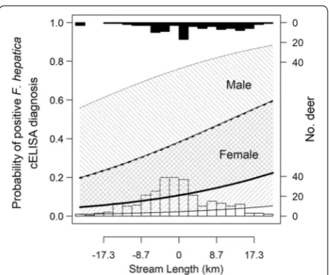
The total variation in diagnostic probabilities explained by the combination of random and fixed effects was 28% (conditional R2_{). Only 13% (marginal R}2_{) of the variation} was explained by fixed effects alone and only one habi-tat related fixed effect parameter estimate was non-zero (Table 3). Here, a strong positive association occurred for stream length (Fig. 4). We found no non-zero associa-tions between diagnosis and land cover or meteorological variables.

Of the collinear host-related variables (sex and date culled), the model portioned the strongest non-zero effect size to sex. Here, males were more likely to be diag-nosed positive, which equated to an odds ratio relative to females of 5.12 (95% CI: 1.83–15.22) (Table 3). The model also assigned a further (but weaker) non-zero parameter estimate to a positive association with the number of days into the hunting season.

In terms of model prediction efficacy, AUC for the training data indicated useful accuracy (0.78; 95% boot-strap CI: 0.73–0.83). Using the training data and a cut-off probability of > 0.50 as an indicator of positive diagnosis (as predicted by the model), we calculated model sensi-tivity of 0.23 (95% bootstrap CI: 0.15–0.32) and specific-ity of 0.96 (95% bootstrap CI: 0.94–0.98).

Discussion

This study explored the associations between habitat and host related variables and F. hepatica diagnosis in wild red deer in the Scottish Highlands during two sampling years, 2012–2013 and 2013–2014. In terms of habitat var-iation, we revealed that cELISA based estimates of expo-sure are most strongly (and positively) associated with home range stream length. Contrary to our expectations, diagnosis did not vary with the annual number of days during which the temperature threshold for F. hepatica development was exceeded, nor did diagnosis associ-ate with variation in annual rainfall. Inherent collinear-ity between sex and sampling date inflated the variance of our model coefficient estimates for these variables, yet we found a strong association between diagnosis and

when using held-out 2012–2013 data, which highlighted the moderate but nonetheless useful transferability of our findings.

Fasciola hepatica diagnoses in relation to habitat and host variation

The relationship between stream length and F. hepatica diagnosis might reflect a greater availability of tolerable habitat for an intermediate host; even though the streams themselves are not necessarily occupied by those inter-mediate hosts. Surveys of macro invertebrates in Scottish Highland running freshwaters reveal that G. truncatula is

typically absent from streams; i.e. it was found in just one river in our study region between 2005 and 2007 [55, 56]. Notwithstanding possible systematic reasons for this lack of detection (i.e. related to kick sampling methods), it is more plausible that G. truncatula simply occurs in habi-tats close to streams rather than in the streams them-selves [57]. Indeed, a range of permanent and temporary small water bodies are tolerable for G. trunctula [58].

The lack of association between mean annual rainfall and/or number of development days, and, probability of F. hepatica diagnosis, might be a consequence of the large uncertainties that accompany interpolations of meteoro-logical data across topographically diverse regions. In a UK context, grid data is spatially interpolated from station data using a linear relationship between altitude and tem-perature [59, 60]. However, the 5 × 5 km grid used is likely to be of insufficient scale to resolve differences in weather experienced by deer within a single estate which may only span a maximum of around 15 km (at its greatest extent). Of course, meteorological suitability for F. hepatica and its intermediate snail hosts does not necessarily directly imply infection of definitive hosts. Fasciola hepatica must first be present, either endemically or introduced (perhaps through livestock imports, as has occurred in historically F. hepatica-free areas in the south east of GB; [61]). Addi-tionally, one must consider the tolerability of land cover for intermediate hosts. In this regard, G. truncatula is appar-ently unable to tolerate blanket bog environments (e.g. in Orkney; [10]), which cover large areas of the Scottish Highlands. We note that average annual rainfall total and mean temperature are associated with F. hepatica related condemnation of cattle liver at slaughter in Scotland [62], but that the distribution of sampled farms in the Scottish Highlands is concentrated at the coastlines; hence, the rainfall experience by cattle is unlikely to be as great as experienced by the deer in our study, which occupy higher ground primarily inland from the coast.

Table 2 Summary of host and habitat characteristics for wild red deer (Cervus elaphus) from estimated 2 km radius home ranges in the Scottish Highlands. Units in which ranges are expressed are indicated in parentheses in the explanatory variables column

Abbreviations: F, female deer; M, male deer

Notes: Annual development days were defined as the total number of days per year with mean air temperature exceeding 10°C. Mean annual rainfall total and mean annual development days were calculated using data from the 5 years immediately preceding each sampling season

Explanatory variable 2012–2013 2013–2014

M (n= 173) F (n= 116) M (n= 211) F (n= 179)

Days into season (days) 33–112 114–230 39–112 113–228

Stream length (km) 24.7–62.6 22.2–64.9 24.1–64.5 20.8–65.2

Blanket bog (%) 0–86.8 0–72.4 0–90.5 0–81.4

Heather moor (%) 13.2–99.9 18.6–94.5 8.2–97.6 10–99.7

Smooth grassland (%) 0–42.5 0–40.2 0–39.3 0–50.6

Mean annual rainfall total (mm) 1053–3363 1005–3715 1002–3564 1013–3658

Mean annual development days (days) 35.5–163.9 35.5–157.3 40–157.7 37–156.9

Table 3 Fixed effect parameter estimates for a binomial (logit link) generalised linear mixed effect model describing the probability of positive Fasciola hepatica coproantigen ELISA diagnosis for faecal samples of wild Scottish red deer (Cervus

elaphus) (n= 390) in relation to host and habitat within 2 km

radius estimated home range

Notes: Habitat data in terms of home range percentage land cover [28], meteorology [20] and topographically derived stream length [25, 26] were mean-centred and scaled to standard deviation units prior to logistic regression against binary cELISA diagnoses. Values in parentheses represent 95% (profile) confidence intervals. Annual development days were defined as the total number of days per year with mean air temperature exceeding 10 °C. Mean annual rainfall total and mean annual development days were calculated using data from the 5 years immediately preceding sampling season 2013–2014

Fixed effect parameter Estimate (95% CI)

(Intercept) − 2.12 (− 3.076 to − 1.198)

Sex 1.634 (0.603–2.722)

Days into season 0.521 (0.016–1.037)

Stream length 0.349 (0.047–0.658)

Mean annual rainfall total 0.148 (− 0.421 to 0.683) Mean annual development days 0.266 (− 0.179 to 0.708)

Blanket bog 0.115 (− 0.437 to 0.665)

Heather moor 0.223 (− 0.193 to 0.653)

The lack of relationship between F. hepatica diagno-sis and the presence of smooth grassland (or indeed any other land cover) within the deer home ranges here, might be an indication that G. truncatula has a wide tolerance for other habitats (e.g. in terms of soil pH; as also noted in Orkney; [10]). Alternatively, G. trunca-tula might not be the only important intermediate host, and intermediate hosts that are more tolerant of upland environments may occupy a more prominent role in the F. hepatica life-cycle in the Scottish Highlands than is typical in lowland habitats. This latter hypothesis is sup-ported by 19 records of a less common host, R. balthica [19, 63, 64], identified during kick sampling of streams in peatland and heather dominated habitats [55, 56].

While we could not disentangle associations between sex and sampling date, their relatively strong explanatory contribution (here mostly weighted to a large effect size for sex; when compared to those estimated for land cover and meteorological variables) alluded to at least one or the other’s substantial association with F. hepatica diag-noses. Where these effects have been disentangled using year-round coprological surveys of male and female wild

Scottish red deer [16], male biased F. hepatica diagno-sis has not been observed, whereas seasonal variation in prevalence and intensity of F. hepatica diagnoses appears strong. In this case, significantly lower prevalence and intensity of infection (faecal egg counts) occurred in adults of both sexes during winter (i.e. our female sampling sea-son) [16]. The fact that any temporal signature is detect-able despite the lack of anthelmintic treatment of wild deer begs further questions. For example, to what extent are diagnoses during a given hunting season a reflection of infection in the previous year, as opposed to lifetime bur-den? Or, do our observations reflect temporal changes in F. hepatica coproantigen detectability, perhaps related to physiological changes such as fatty liver, which occurs in males following the breeding season [65]? If, conversely, our coefficient estimates reflect a true underlying male biased parasitism, this would reflect observations in other wild ungulates (e.g. lungworm (Protostrongylidae) in red deer [66] and chamois (Rupicapra rupicapra rupicapra) [67]).

Variance explained and transferability of findings

We were aware that the explanatory power of regression type analyses inevitably increases with the addition of variables, so we had to ensure we did not overparameter-ize and thus overfit our model. Various methods to assess the transferability of model findings related to F. hepatica exposure in livestock and environmental variability have been explored. For example, using linear regression and a range of explanatory environmental variables, Howell et  al. [8] used comparisons of R2 _{between training and} test data to assess transferability, whereby their fitted model explained 37% of differences in F. hepatica expo-sure among farms in England and Wales, which notably increased to 49% using held-out test data. In Northern Ireland, transferability of findings has been assessed by constructing multiple models and comparing their coef-ficient estimates, i.e. identifying the most parsimonious model for each year within their study (based on lowest value of the Akaike’s information criterion). There, Byrne et al. [68] noted that separate models for 2011, 2012 and 2013 data that described variance in a binary response variable (F. hepatica severity based on cattle herd level prevalence) inconsistently retained long-term weather variables. In the present study, the transferability of our model was encouraging owing to only a slight reduction in point estimates of prediction efficacy for our model when applied to held-out data from 2012–2013. Never-theless, this demonstrates that our estimate of explained variance (R2 _{of 28%) might be marginally over-optimistic.}

The amount of variance attributable to unmeasured differences among estates warrants further attention; in this regard, a range of finer scale habitat covariates might Fig. 4 Visual representation of a generalised linear mixed effect

model parameter estimate describing probability of positive

improve the explanatory power of these models. However, it is perhaps management related factors (such as supplemen-tary feeding, which is practiced widely in the Scottish High-lands [69]), that could influence (amongst other factors) deer habitat use and spatial aggregation [70] and might thus facilitate the greatest gains in model performance. Unfenced livestock, which are also present in some Scottish Highland hunting estates, are also feasible contributors to F. hepatica infection risk for wild deer (and vice versa).

Estate scale non‑independence in diagnoses

Any spatial (e.g. Fig. 3) and temporal dependencies in the raw data were accounted for by our model specification. However, in terms of spatial dependency, our (induced) intraclass compound symmetry correlation structure demonstrated that diagnoses within sites were not neces-sarily independent from each other. While a compound symmetry structure implies that spatial dependencies act equally as strongly over short distances as they do over tens of kilometres (e.g. between two animals on opposite extremities of the same hunting estate), this is a simplified picture. Because of a lack of significant Moran’s I or spatial patterns in residuals, we did not attempt to explicitly quan-tify distances over which underlying epidemiological neigh-bourhood scale processes act (i.e. between animals with overlapping home ranges). However, should future surveil-lance data be of sufficiently high resolution, it might be pos-sible to gain an insight into such processes, as advocated in terms of spatial [13] and temporal dependencies in F. hepat-ica infection and indeed for parasitology in general [71].

Limitations

Ideally, our surveillance data would have mirrored a fully-crossed (full-factorial) randomized block experimental design insofar as all values for host and environmental explanatory variables would have been replicated on all sampled hunting estates [72]. However, differences in management practices meant that some estates (for exam-ple) culled females until late December, while others con-tinued culling until mid-February. Furthermore, we did not include finer scale habitat information, such as Juncus spp. infested grassland, which is present in LCS88 and is a useful indicator of G. truncatula presence [73], because it was not present on all estates. While our random intercept approach went some way to dealing with our partially-crossed design, it left considerable room for influential estates, i.e. estates for which exclusive combinations of explanatory and response variable values were present. For example, NA estate had the greatest influence on the date culled parameter because more than half of the diagnoses were positive and samples at NA were collected an aver-age of 20 days later than the next latest sampling estate, CO. Similarly, a positively diagnosed sample at AR had

the greatest influence on the smooth grassland parameter (albeit ultimately a zero-effect parameter) owing to the large proportion of smooth grassland in its home range.

The effective sample size of our model training data must be considered in relation to two aspects of statistical power. First, for an exploratory study such as ours, power to detect a hypothesised effect size for an explanatory vari-able is calculated from the combined influence of the mag-nitude of effect size, the number of samples per hunting estate, the number of estates, and the properties of the var-iable of interest (e.g. bounded land cover proportion; con-tinuous stream length). Here, our study detected a positive association between F. hepatica diagnosis and the length of stream within red deer home range. Were this effect size to be arbitrarily classified as “medium” (for example, owing to a coefficient estimate of ~0.4 standard deviation units), it is important to note that the size of this effect might be overestimated (positively biased) if the power of the design to identify such effects is low (e.g. as demonstrated by sim-ulation studies [74]). Regardless, the confidence intervals (Table 3 and Fig. 4), serve as a warning as to the precision of this effect size estimate.

The second aspect of statistical power to consider is the possibility of Type II error, i.e. does percentage of smooth grassland occupying home ranges of red deer really not associate with the probability of F. hepatica diagnosis, or did our design have insufficient power to detect an effect? Relative to stream length, it appears likely that any underlying association between F. hepatica diagnosis and smooth grassland is small. To provide an indication of possible Type II error, we retrospectively estimated the power of our analysis (using the simr R package [75]) to detect a defined small effect size (0.2 SD) for grassland. The resulting estimate of 32% power based on 250 simu-lations is undesirable, but nevertheless must be consid-ered in the context of the aim of the study. Our study was exploratory and dependent on sample collections from wild deer, rather than based on controlled field manipu-lation whereby a design could test for particular sizes of effects (e.g. small, ≤ 0.2 SD), though tools and guidance for a priori simulation based power analysis for GLMMs have become available since study [75, 76]); thus, while our results should be considered inconclusive with regards to a possible small association between smooth grassland percentage and F. hepatica diagnosis, we can nevertheless have confidence that had there been a larger effect (e.g. 0.5 SD, again tested using the simr R package [75]), we had 93% power to detect it.

Scottish island (or coastal) dwelling female red deer may be relatively smaller (at mean ± SD; 1.3 ± 1.6 km2_{) than our} estimates [78]. In addition, our data collection spanned only seven months of each sampling year and it is unclear whether cull locations accurately represent the centroid of each individual’s annual home range. This is because red deer have different winter and summer ranges depend-ing on (for example) sex and broad-scale habitat type [79]. While more precise knowledge of habitat use by indi-vidual deer might have improved our model performance (i.e. prediction efficacy and transferability), it is neverthe-less worth noting that Scottish red deer are neverthe-less selective in terms of grazing patch sizes than other herbivores such as sheep, which tend to prefer smaller patches [80]; thus, proportions of immediate surrounding land cover (as quantified herein) might indeed usefully describe variation in wild red deer habitat related to (for example) a greater probability of encountering infective metacercariae.

The consequences of over- or underestimating red deer home ranges in this study might introduce bias to param-eter estimates. For example, if female ranges were over-estimated, we would in turn be overestimating the length of stream in their habitat. As such, fewer samples from females than males were diagnosed positive; therefore, it is possible that a portion of the negative diagnoses clus-tered with relatively long home range stream lengths (e.g. in Fig. 4) were derived from female samples (see similar ranges for both sexes in Table 2) and may therefore be deflating the effect size. This is just one example, but it is important to be aware of the consequences of inaccurate home range estimates in exploratory studies of this type.

Finally, we note that owing to the sensitivity of the cELISA, a portion of positive infections will have been missed and this is likely to have diluted the strength of effects identified by our model.

Conclusions

The probability of F. hepatica diagnosis in Scottish Highland deer is ostensibly associated with variation between the sexes and/or the date on which samples are collected, and the length of streams in an individu-al’s home range. The association between stream length and diagnosis might be related to the suitability of habi-tat for intermediate snail hosts (with stream length per-haps acting as a useful proxy related to the likelihood of exposure and thus infection). However, the prevail-ing importance of various possible intermediate host species requires further investigation. Greater odds of positive diagnosis in males relative to females reflects observations in other ungulates; and, whilst sex was inherently correlated with sampling date (thus inflat-ing the variances associated with our model coeffi-cient estimates for these two variables), this served to

demonstrate that the association between at least one of these variables and diagnosis of F. hepatica is strong. While we did not identify any non-zero relationship between meteorological variables and probability of diagnosis, we attribute this (in part) to uncertainty in the modelling of climate data in topographically diverse regions. The statistical power of the model was prob-ably limited by a deflated effective sample size and as such we advocate a wider geographical sampling protocol (no more samples per site, but more sites). More than half of the explained variation in diagnosis probability was attributable to unquantified overarch-ing differences among samploverarch-ing sites, which highlights significant gaps in basic data (i.e. regarding habitat and deer management), and in our understanding. Exten-sions to explore neighbourhood-scale processes affect-ing F. hepatica transmission could be applied to this study, such as intensive sampling in areas with low F. hepatica prevalence. We would then advocate a simi-lar approach to that taken here, in which confidence in the transferability of findings should be mediated by an evaluation of any explanatory model in terms of predic-tion efficacy and transferability.

Supplementary information

Supplementary information accompanies this paper at https ://doi. org/10.1186/s1307 1‑019‑3782‑3.

Additional file 1: Figure S1. Standardized residuals vs predictors. This figure revealed no strong evidence of non‑linear relationships between predictors and response (probability of diagnosis). The plot was produced using the plotResiduals() function in the DHARMa R package [43]. Additional file 2: Residuals vs time (mean‑centred and standard devia‑ tion scaled days after 1st July 2012) (left), autocorrelation function (ACF) for diagnostic data vs time lags of up to 25 days for model residuals (right). The dashed lines in the ACF plot illustrate the magnitude of the autocor‑ relation function beyond which autocorrelation is statistically significant. Therefore, this figure reveals borderline residual temporal autocorrelation at 1‑ and 8‑days lag; neither of which we consider to be of concern. The figure was produced using the testTemporalAutocorrelation() function in the DHARMa R package [43] and the acf() function in the ncf R package [81].

Additional file 3: Figure S3. Spatially plotted residuals. This figure revealed no evidence of residual spatial autocorrelation and was created using an adaptation of the testSpatialAutocorrelation() function in the DHARMa R package [43]. The colour scale illustrates the magnitude of scaled simulated uniform residuals.

Abbreviations

ACF: autocorrelation function; AL: Alladale; AP: Applecross Trust; AR: Ardna‑ murchan; AT: Altnaharra; AUC : area under the receiver operating characteristic curve; BA: Badanloch; BL: Ben Loyal; cELISA: coproantigen enzyme‑linked immunosorbent assay; CO: Conaglen; DTM: Digital Terrain Model; GB: Great Britain; GLMM: Generalised Linear Mixed Effect Model; ICC: intraclass correla‑ tion coefficient; LCS88: Land Cover Scotland 1988; NA: North Harris Trust and Aline; (Q)GIS: (Quantum) Geographic Information System; ST: Strathconon.

Acknowledgements

Ardnamurchan, Badanloch, Ben Loyal, Conaglen, North Harris Trust and Strath‑ conon estates for their diligent sample collection, without whom this study would not have been possible.

Authors’ contributions

ASF and MAT conceived and designed the study. ASF, GM, DKG‑G conducted the laboratory analyses. ASF conducted the statistical analyses and wrote the manuscript with contributions from MAT, RNZ and PJS. All authors read and approved the final manuscript.

Funding

ASF’s studentship was funded by the Highlands and Islands of Scotland European Social Fund [2007UK051PO001] 2007–2013 programme. Funding for contributions by GM, PJS and RNZ was obtained from the Scottish Govern‑ ment’s Rural and Environmental Science and Analytical Services Division. Funding for DKG‑G’s contribution was obtained from the Peter Doherty PhD studentship awarded by the Moredun Foundation. The funders had no role in study design, data collection and analysis, decision to publish, or preparation of the manuscript.

Availability of data and materials

Data supporting the conclusions of this article are provided within the article and its additional files. The datasets analysed during the present study are available from the corresponding author upon reasonable request.

Ethics approval and consent to participate

No ethics approval was required for this study. See Materials and Methods section of [17] for details.

Consent for publication Not applicable.

Competing interests

The authors declare that they have no competing interests.

Author details

1 _{Environmental Research Institute, North Highland College, University} of the Highlands and Islands, Castle Street, Thurso KW14 7JD, UK. 2 _Present Address: Marine Institute, Furnace, Newport, Co. Mayo, Ireland. 3 _Institute of Biodiversity Animal Health and Comparative Medicine, University of Glas‑ gow, Garscube Campus, Glasgow G61 1QH, UK. 4 _{Moredun Research Institute,} Pentlands Science Park, Bush Loan, Penicuik EH26 0PZ, UK. 5 _{Present Address:} Sydney School of Veterinary Science, University of Sydney, Camden NSW 2570, Australia.

Received: 11 June 2019 Accepted: 30 October 2019

References

1. Caminade C, Van Dijk J, Baylis M, Williams D. Modelling recent and future climatic suitability for fasciolosis in Europe. Geosp Health. 2015;9:301–8. 2. APHA. Veterinary investigation diagnosis analysis reports archive: yearly trends in cattle and sheep; 1996–2003, 2001–2008, 2009–2016. Animal, Plant Health Agency, UK Government; 2016. Pre‑ 2013: https ://webar chive .natio nalar chive s.gov.uk/20140 30603 5701/http://www.defra .gov. uk/ahvla ‑en/categ ory/publi catio ns/disea se‑surv/vida/. Post 2013: https ://www.gov.uk/gover nment /publi catio ns/veter inary ‑inves tigat ion‑diagn osis‑analy sis‑vida‑repor t‑2016. Accessed 2 Oct 2017.

3. van Dijk J, Sargison ND, Kenyon F, Skuce PJ. Climate change and infectious disease: helminthological challenges to farmed ruminants in temperate regions. Animal. 2010;4:377.

4. Böhm M, White PC, Daniels MJ, Allcroft DJ, Munro R, Hutchings MR. The health of wild red and sika deer in Scotland: an analysis of key endoparasites and recommendations for monitoring disease. Vet J. 2006;171:287–94.

5. Charlier J, Vercruysse J, Morgan E, Van Dijk J, Williams DJL. Recent advances in the diagnosis, impact on production and prediction of Fasciola hepatica in cattle. Parasitology. 2014;141:326–35.

6. Hawkins CD, Morris RS. Depression of productivity in sheep infected with Fasciola hepatica. Vet Parasitol. 1978;4:341–51.

7. Hickey GL, Diggle PJ, McNeilly TN, Tongue SC, Chase‑Topping ME, Wil‑ liams DJ. The feasibility of testing whether Fasciola hepatica is associated with increased risk of verocytotoxin producing Escherichia coli O157 from an existing study protocol. Prev Vet Med. 2015;119:97–104.

8. Howell A, Baylis M, Smith R, Pinchbeck G, Williams D. Epidemiology and impact of Fasciola hepatica exposure in high‑yielding dairy herds. Prev Vet Med. 2015;121:41–8.

9. Browning L, Hawkins G, Allison L, Bruce R. National outbreak of Escheri-chia coli 0157 phage type 32 in Scotland: report to the incident manage‑ ment team. Glasgow: Health Protection Scotland; 2016.

10. Heppleston PB. Life history and population fluctuations of Lymnaea trun-catula (Mull.), the snail vector of fascioliasis. J Appl Ecol. 1972;9:235–48. 11. Rowcliffe SA, Ollerenshaw CB. Observations on the bionomics of the egg

of Fasciola hepatica. Ann Trop Med Parasit. 1960;54:172–81.

12. Ollerenshaw C, Rowlands W. A method of forecasting the incidence of fascioliasis in Anglesey. Vet Rec. 1959;71:591–8.

13. Bennema SC, Ducheyne E, Vercruysse J, Claerebout E, Hendrickx G, Charlier J. Relative importance of management, meteorological and environmental factors in the spatial distribution of Fasciola hepatica in dairy cattle in a temperate climate zone. Int J Parasitol. 2011;41:225–33. 14. UK Met Office. UK climate 2017. https ://www.metoffi ce.gov.uk/publi c/

weath er/clima te/. Accessed 20 Nov 2017.

15. Ollerenshaw CB. The approach to forecasting the incidence of fascioliasis over England and Wales 1958–1962. Agric Meteorol. 1966;3:35–53. 16. Albery GF, Kenyon F, Morris A, Morris S, Nussey DH, Pemberton JM. Sea‑

sonality of helminth infection in wild red deer varies between individuals and between parasite taxa. Parasitology. 2018;145:1410–20.

17. French AS, Zadoks RN, Skuce PJ, Mitchell G, Gordon‑Gibbs DK, Craine A, et al. Prevalence of liver fluke (Fasciola hepatica) in wild red deer (Cervus elaphus): coproantigen ELISA is a practicable alternative to faecal egg counting for surveillance in remote populations. PLoS ONE. 2016;11:e0162420.

18. Fox NJ, White PCL, McClean CJ, Marion G, Evans A, Hutchings MR. Predicting impacts of climate change on Fasciola hepatica risk. PLoS ONE. 2011;6:e16126.

19. Relf V, Good B, McCarthy E, de Waal T. Evidence of Fasciola hepatica infec‑ tion in Radix peregra and a mollusc of the family Succineidae in Ireland. Vet Parasitol. 2009;163:152–5.

20. UK Met Office, Hollis D, McCarthy M. Met Office gridded and regional land surface climate observation datasets: Centre for Environmental Data Analysis, 2017. http://catal ogue.ceda.ac.uk/uuid/87f43 af9d0 2e42f 48335 1d79b 3d616 2a. Accessed 24 Sept 2017.

21. R Core Team. R: a language and environment for statistical computing. Vienna, Austria: R Foundation for Statistical Computing; 2015. 22. Wickam H, Hester J, Francois R. Readr: read rectangular text data. 2017.

https ://CRAN.R‑proje ct.org/packa ge=readr .

23. Wickam H. Reshaping data with the reshape package. J Stat Softw. 2007;21:1–20.

24. Dowle M, Srinivasan A. Data.table: extension of ‘data.frame‘. 2017. https :// CRAN.R‑proje ct.org/packa ge=data.table .

25. CEDA. Landmap; GetMapping (2014): GetMapping 5m resolution Digital Terrain Model (DTM) for Scotland. Oxford: NERC Earth Observation Data Centre; 2017. http://catal ogue.ceda.ac.uk/uuid/fe892 26774 e191a 45ea4 a17c4 d64ce a1. Accessed 26 Jun 2017.

26. Murphy PNC, Ogilvie J, Meng F‑R, Arp P. Stream network modelling using lidar and photogrammetric digital elevation models: a comparison and field verification. Hydrol Process. 2008;22:1747–54.

27. ESRI. ArcGIS desktop. Redlands: Environmental Systems Research Insti‑ tute; 2011.

28. The James Hutton Institute. Land Cover Scotland (LCS) 1988 ‑ Data‑ sets. 1992. https ://data.gov.uk/datas et/land‑cover ‑scotl and‑lcs‑1988;

http://sedsh 127.sedsh .gov.uk/Atom_data/ScotG ov/Zippe dShap efile s/ SG_LandC overS cotla nd_1988.zip. Accessed 28 Oct 2015.

29. QGIS Development Team. QGIS. 2017. http://www.qgis.org/. Accessed 1 Mar 2018.

30. Bivand R, Rundel C. rgeos: interface to geometry engine – open source (‘GEOS’). 2019. https ://CRAN.R‑proje ct.org/packa ge=rgeos .

32. Hijmans RJ. Raster: Geographic data analysis and modeling. 2019. https :// CRAN.R‑proje ct.org/packa ge=raste r.

33. Bivand R, Keitt T, Rowlingson B. Rgdal: bindings for the ‛geospatial’ data abstraction library. 2017. https ://CRAN.R‑proje ct.org/packa ge=rgdal . 34. Schnute JT, Boers N, Haigh R. PBSmapping: mapping fisheries data and

spatial analysis tools. 2017. https ://CRAN.R‑proje ct.org/packa ge=PBSma pping .

35. Team R. RStudio: integrated development for R. Boston, MA; 2015. http:// www.rstud io.com/

36. Zuur AF, Ieno EN. A protocol for conducting and presenting results of regression‑type analyses. Methods Ecol Evol. 2016;7:636–45.

37. Elston DA, Moss R, Boulinier T, Arrowsmith C, Lambin X. Analysis of aggrega‑ tion, a worked example: numbers of ticks on red grouse chicks. Parasitology. 2001;122:563–9.

38. Brunsdon C, McClatchey J, Unwin D. Spatial variations in the average rainfall‑ altitude relationship in Great Britain: an approach using geographically weighted regression. Int J Climatol. 2001;21:455–66.

39. Roberts DR, Bahn V, Ciuti S, Boyce MS, Elith J, Guillera‑Arroita G, et al. Cross‑validation strategies for data with temporal, spatial, hierarchical, or phylogenetic structure. Ecography. 2017;40:913–29.

40. Wenger SJ, Olden JD. Assessing transferability of ecological models: an underappreciated aspect of statistical validation: Model transferability. Methods Ecol Evol. 2012;3:260–7.

41. Bates D, Maechler M, Bolker B, Walker S. Fitting Linear Mixed‑Effects Models using lme4. J Stat Softw. 2015;67:1–48.

42. Peterson BG, Carl P. PerformanceAnalytics: econometric tools for perfor‑ mance and risk analysis. 2014. https ://CRAN.R‑proje ct.org/packa ge=Perfo rmanc eAnal ytics .

43. Hartig F. DHARMa: Residual diagnostics for hierarchical (multi‑level /mixed) regression models. 2017. https ://CRAN.R‑proje ct.org/packa ge=DHARM a. 44. Robin X, Turck N, Hainard A, Tiberti N, Lisacek F, Sanchez J‑C, et al. pROC: an

open‑source package for R and S+ to analyze and compare ROC curves. BMC Bioinformatics. 2011;12:77.

45. Swets JA. Measuring the accuracy of diagnostic systems. Science. 1988;240:1285–93.

46. Zuur AF, Ieno EN, Walker NJ, Saveliev AA, Smith GM. Mixed effects models and extensions in ecology with R. New York: Springer; 2009.

47. Wu S, Crespi CM, Wong WK. Comparison of methods for estimating the intraclass correlation coefficient for binary responses in cancer prevention cluster randomized trials. Contemp Clin Trials. 2012;33:869–80.

48. Peduzzi P, Concato J, Kemper E, Holford TR, Feinstein AR. A simulation study of the number of events per variable in logistic regression analysis. J Clin Epidemiol. 1996;49:1373–9.

49. Lüdecke D. Sjstats: statistical functions for regression models. 2018. https :// CRAN.R‑proje ct.org/packa ge=sjsta ts.

50. Nieuwenhuis R, Te Grotenhuis M, Pelzer B. Influence.ME: tools for detecting influential data in mixed effects models. R J. 2012;4:38–47.

51. Nakagawa S, Schielzeth H. A general and simple method for obtain‑ ing R2 _{from generalized linear mixed‑effects models. Methods Ecol} Evol. 2013;4:133–42.http://onlin elibr ary.wiley .com/doi/10.1111/j.2041‑ 210x.2012.00261 .x/abstr act

52. Lefcheck JS. piecewiseSEM: Piecewise structural equation modeling in R for ecology, evolution, and systematics. Methods Ecol Evol. 2016;7:573–9. 53. Stubben CJ, Milligan BG. Estimating and analyzing demographic models

using the popbio package in R. J Stat Softw. 2007;22:1–23.

54. Dormann CF, Elith J, Bacher S, Buchmann C, Carl G, Carré G, et al. Collinearity: a review of methods to deal with it and a simulation study evaluating their performance. Ecography. 2013;36:27–46.

55. SEPA. Scottish river macro‑invertebrate records from 2007 collected by SEPA. Scottish Environment Protection Agency; 2012. https ://doi.org/10.15468 / l82tv b. Accessed 14 Mar 2017.

56. SEPA. River macroinvertebrate data for 2005 and 2006. Scottish Environment Protection Agency; 2012. https ://doi.org/10.15468 /knxcq i. Accessed 14 Mar 2017.

57. Charlier J, Bennema SC, Caron Y, Counotte M, Ducheyne E, Hendrickx G, et al. Towards assessing fine‑scale indicators for the spatial transmission risk of Fasciola hepatica in cattle. Geosp Health. 2011;5:239–45.

58. Charlier J, Soenen K, Roeck ED, Hantson W, Ducheyne E, Coillie FV, et al. Longitudinal study on the temporal and micro‑spatial distribution of Galba truncatula in four farms in Belgium as a base for small‑scale risk mapping of Fasciola hepatica. Parasit Vectors. 2014;7:528.

59. Hudson G, Wackernagel H. Mapping temperature using kriging with external drift: theory and an example from Scotland. Int J Climatol. 1994;14:77–91.

60. Perry M, Hollis D. The generation of monthly gridded datasets for a range of climatic variables over the United Kingdom. Exeter: Met Office; 2004. 61. Pritchard GC, Forbes AB, Williams DJL, Salimi‑Bejestani MR, Daniel RG. Emer‑

gence of fasciolosis in cattle in East Anglia. Vet Rec. 2005;157:578–82. 62. Innocent GT, Gilbert L, Jones EO, McLeod JE, Gunn G, McKendrick IJ, Albon

SD. Combining slaughterhouse surveillance data with cattle tracing scheme and environmental data to quantify environmental risk factors for liver fluke in cattle. Front Vet Sci. 2017;4:65.

63. Caron Y, Martens K, Lempereur L, Saegerman C, Losson B. New insight in lym‑ naeid snails (Mollusca, Gastropoda) as intermediate hosts of Fasciola hepatica (Trematoda, Digenea) in Belgium and Luxembourg. Parasit Vectors. 2014;7:66. 64. Rondelaud D, Titi A, Vignoles P, Mekroud A, Dreyfuss G. Adaptation of

Lymnaea fuscus and Radix balthica to Fasciola hepatica through the experi‑ mental infection of several successive snail generations. Parasit Vectors. 2014;7:296.

65. Zomborszky Z, Husvéth F. Liver total lipids and fatty acid composition of shot red and fallow deer males in various reproduction periods. Comp Biochem Phys A. 2000;126:107–14.

66. Vicente J, Höfle U, Fernández‑De‑Mera IG, Gortazar C. The importance of parasite life history and host density in predicting the impact of infections in red deer. Oecologia. 2007;152:655–64.

67. Hoby S, Schwarzenberger F, Doherr MG, Robert N, Walzer C. Steroid hormone related male biased parasitism in chamois, Rupicapra rupicapra rupicapra. Vet Parasitol. 2006;138:337–48.

68. Byrne AW, McBride S, Lahuerta‑Marin A, Guelbenzu M, McNair J, Skuce RA, et al. Liver fluke (Fasciola hepatica) infection in cattle in Northern Ireland: a large‑scale epidemiological investigation utilising surveillance data. Parasit Vectors. 2016;9:209.

69. Putman RJ, Staines BW. Supplementary winter feeding of wild red deer Cervus elaphus in Europe and North America: justifications, feeding practice and effectiveness. Mammal Rev. 2004;34:285–306.

70. Jerina K. Roads and supplemental feeding affect home‑range size of Slove‑ nian red deer more than natural factors. J Mammal. 2012;93:1139–48. 71. Pollitt LC, Reece SE, Mideo N, Nussey DH, Colegrave N. The problem of auto‑

correlation in parasitology. PLoS Pathog. 2012;8:e1002590.

72. Schielzeth H, Nakagawa S. Nested by design: model fitting and interpreta‑ tion in a mixed model era. Methods Ecol Evol. 2013;4:14–24.

73. Rondelaud D, Hourdin P, Vignoles P, Dreyfuss G, Cabaret J. The detection of snail host habitats in liver fluke infected farms by use of plant indicators. Vet Parasitol. 2011;181:166–73.

74. Johnson PCD, Barry SJE, Ferguson HM, Müller P. Power analysis for general‑ ized linear mixed models in ecology and evolution. Methods Ecol Evol. 2015;6:133–42.

75. Green P, MacLeod CJ. SIMR: an R package for power analysis of generalized linear mixed models by simulation. Methods Ecol Evol. 2016;7:493–8. 76. Kain MP, Bolker BM, McCoy MW. A practical guide and power analysis for

GLMMs: detecting among treatment variation in random effects. PeerJ. 2015;3:e1226.

77. Catt DC, Staines BW. Home range use and habitat selection by red deer ( Cer-vus elaphus) in a Sitka spruce plantation as determined by radio‑tracking. J Zool. 1987;211:681–93.

78. Froy H, Börger L, Regan CE, Morris A, Morris S, Pilkington JG, et al. Declining home range area predicts reduced late‑life survival in two wild ungulate populations. Ecol Lett. 2018;21:1001–9.

79. Reinecke H, Leinen L, Thißen I, Meißner M, Herzog S, Schütz S, et al. Home range size estimates of red deer in Germany: environmental, individual and methodological correlates. Eur J Wildlife Res. 2013;60:237–47.

80. Hester AJ, Gordon IJ, Baillie GJ, Tappin E. Foraging behaviour of sheep and red deer within natural heather/grass mosaics. J Appl Ecol. 1999;36:133–46. 81. Bjornstad ON. Ncf: Spatial nonparametric covariance functions. 2016. https

://CRAN.R‑proje ct.org/packa ge=ncf.

Publisher’s Note