simulink environment
.
White Rose Research Online URL for this paper:
http://eprints.whiterose.ac.uk/9782/
Article:
Holloway, A.J., Tozer, R.C. and Stone, D.A. (2009) A physically based fluorescent lamp
model for a SPICE or a simulink environment. IEEE Transactions on Power Electronics, 24
(9). pp. 2101-2110. ISSN 0885-8993
https://doi.org/10.1109/TPEL.2009.2020901
[email protected] https://eprints.whiterose.ac.uk/ Reuse
Unless indicated otherwise, fulltext items are protected by copyright with all rights reserved. The copyright exception in section 29 of the Copyright, Designs and Patents Act 1988 allows the making of a single copy solely for the purpose of non-commercial research or private study within the limits of fair dealing. The publisher or other rights-holder may allow further reproduction and re-use of this version - refer to the White Rose Research Online record for this item. Where records identify the publisher as the copyright holder, users can verify any specific terms of use on the publisher’s website.
Takedown
If you consider content in White Rose Research Online to be in breach of UK law, please notify us by
IEEE TRANSACTIONS ON POWER ELECTRONICS, VOL. 24, NO. 9, SEPTEMBER 2009 2101
A Physically Based Fluorescent Lamp Model
for a SPICE or a Simulink Environment
Arran J. Holloway, Richard C. Tozer, Senior Member, IEEE, and Dave A. Stone
Abstract—This paper describes a method of modeling
fluores-cent lamps. The lamp model can be implemented in all major cir-cuit simulation software packages, an example has been given for SPICE and Simulink. The model is based upon a simplified set of physical equations that gives the model validity over a wider range of operating conditions than current fluorescent lamp SPICE mod-els allow for. The model can be used to model any low-pressure mercury-buffer gas fluorescent lamps by entering key lamp pa-rameters, length, radius, cold-spot temperature, and buffer gas fill pressure. If fill pressure is not known, a default value dependent on lamp radius is used. The model shows good agreement over a wide range of operating frequencies and lamp powers.
Index Terms—Fluorescent lamps, gas discharges, lighting, mod-eling, simulation, SPICE.
I. INTRODUCTION
F
LUORESCENT lamps have played an important role in both industrial and domestic lighting for the last half a cen-tury [1]. With an increasing use of compact fluorescent lamps in homes and new regulation discouraging the use of incandes-cent lamps, their importance for lighting has never been greater. Increasingly, there is a move away from low-frequency mag-netic ballasts toward high-frequency electronic ballasts. The use of high-frequency electronic ballasts increases the lamps efficiency and reduces flicker. Electronic ballasts also allow the lamp to be dimmed and allow control for integrated lighting systems.To assist in the optimization of electronic ballasts, it is nec-essary to have an accurate and computationally efficient model of the fluorescent lamp that is capable of modeling the lamp at different frequencies, dimming levels, and under transient conditions.
The first attempt to create a fluorescent lamp model that was suitable for circuit simulation was undertaken by Francis in 1948 [2]. He suggested that it should be possible to describe a fluorescent lamp with a differential equation based on the fol-lowing three postulates: the rate of increase of electron density is proportional to the current and voltage, the rate of decrease of the electron density is proportional to the electron density, and the instantaneous resistance is inversely proportional to the electron density. Unfortunately, it proved impossible to recon-cile this equation with experimental results. The equation was
Manuscript received October 20, 2008; revised February 11, 2009. Current version published August 21, 2009. Recommended for publication by Associate Editor M. Alonso.
The authors are with the Department of Electronic and Electrical Engi-neering, University of Sheffield, Sheffield S1 3JD, U.K. (e-mail: a.holloway@ sheffield.ac.uk; [email protected]; [email protected]).
Digital Object Identifier 10.1109/TPEL.2009.2020901
later modified in [3] but was still incapable of providing accurate results for high- and low-frequency operation.
Subsequently, with an increasing shift toward high-frequency electronic ballasts, authors concentrated on the high-frequency operation only. Unlike the model proposed by Francis, which at-tempted to use some physical reasoning to construct the model, these models were based purely on empirical behavior. The mod-els were thus applicable only over a narrow range of operating conditions centered on the conditions evident when the required experimental data were collected. They all used a variation in modeling the lamp as a resistor with some form of power depen-dence to model the lamp’s staticV–Icharacteristics [4]–[10].
Mader and Horn [4] attempted to create a more general model that worked for both low and high frequencies. Experimental data were required to obtain the coefficients of the model for different lamp types. The model was capable of modeling the low- and high-frequency behavior but required different coeffi-cients for each case.
The alternative to using such behavioral model is to use a self-consistent collisional radiative (SCCR) model. SCCR mod-els are accurate over a large range of operating conditions and also provide a useful insight into the workings of the discharge, however, although S.C.C.R models have recently been imple-mented in MATLAB [11] and PSPICE [12], the computation time required makes them unattractive to circuit designers.
Recently, there has been growing interest in the construc-tion of a more generic model suitable for circuit simulaconstruc-tion that works over a much greater range of operating conditions and does not require experimental data to be collected. Zissis and Buso [13] were the first to present a model that did not require experimental data using the lamp’s parameters to accommodate different lamps. Although, at low frequencies the shape of the
V–I characteristics matched experimental results, the voltage was approximately 65% of the experimental data while the cur-rent was 50% higher. The model also became purely resistive at high frequencies instead of the characteristic “S” shape seen in theV–Icharacteristic that fluorescent lamps possess. This model focused on finding the electron density only, neglecting the elec-tron mobility. It represented the first step toward the creation of a model based upon a simplified set of physical laws.
More recently, attempts have been made to describe the flu-orescent lamp’s operation using a model of a high-pressure discharge as a framework [14]. This approach gives reasonably accurate results at both high and low frequencies. The model uses a genetic algorithm to tune the model to each lamp type.
This paper presents a model that works over a wide range of operating conditions without the need for experimental data. Conditions where physical relationships are of a type that can
be readily computed, they have been used. Places where the physical processes require iterative solutions, e.g., calculation of electron temperature, a behavioral approximation based on the results of an SCCR model [11] has been employed. We show that this approach leads to a model that predicts well the behavior of lamps over a frequency range 50 Hz to 50 kHz.
The first section covers the physical reasoning behind the model. The second section describes how the model can be implemented. Section three explores the validation of the model over a wide range of possible operating conditions including low frequency (50 Hz) and high frequencies (tens of kilohertzs), over a wide range of power levels. This section also demonstrates the model’s ability to accommodate different lamp geometries without requiring experimental data collection. Section III also illustrates an example of the model being used to simulate a resonant dimming ballast. The simulation of the dimming ballast also investigates the model’s ability to correctly describe step changes in frequency and power.
II. FLUORESCENTLAMPMODEL
The model concentrates on the physical processes that deter-mine the electrical conductivity of the lamp. In determining the lamps conductivity there are two important parameters: the num-ber of electrons available to carry current in the plasma and the mobility of those electrons. The latter plays an important role in determining the lamp’s nonlinear high-frequency behavior. The failure to model the electron mobility in [13] explains why this model becomes resistive prematurely at high frequencies.
We begin by solving the ionization balance equation to deter-mine the number of electrons in the discharge. This is done by finding the rate at which electrons are created through ionization and the rate at which they are removed through recombination with ions at the wall. The electron mobility is then calculated and Ohm’s law is used to calculate the lamp’s conductivity.
As for any fluorescent lamp model, it is necessary to make as-sumptions about the way in which the lamp behaves. This model makes the following assumptions about the lamp’s behavior.
1) The lamp is axially homogenous.
2) Only the positive column has been considered; the elec-trode regions have been ignored.
3) The displacement of species through cataphoresis has not been considered as this happens over a much longer time period than a 50-Hz cycle.
4) The lamp is already ignited, the model does not correctly predict the breakdown stage, however, it is capable of predicting transient events once the lamp is lit.
5) The ions do not play a significant role in the discharge as charge carriers, being much heavier than the electrons. 6) Volume recombination is negligible.
A. Electron Temperature
One method of calculating the electron temperature is to solve the energy balance equation. This uses the idea that the differ-ence between the electrical energy supplied to the lamp and the energy lost through the plasma’s loss mechanisms, such as radi-ation, ionizradi-ation, and thermal losses, allows the average electron
temperature to be calculated. This is the method employed in SCCR models; it has also been used in the semiphysical SPICE model [14]. The problem with solving the energy balance equa-tion is that it requires the calculaequa-tion of the rate of transiequa-tions between all the energy levels, or lumped pseudoenergy states, which is a computationally intense process. To reduce the com-putational intensity of this calculation, an approximation to the power lost through radiation given in [14], is given by
Prad =a2e(−eae/k Te). (1)
This is based upon the use of the Boltzmann factor that ex-presses the probability of an energy state compared to the ground energy state. However, the use of the Boltzmann factor is only suitable for gasses that are in local thermal equilibrium (LTE). In the low-pressure-discharge regime normally found in a fluo-rescent lamp the electrons are typically at a temperature 40 or 50 times greater than the buffer gas and ions, therefore, it is not possible to say that they are in LTE. Results from our SCCR model [15] show that a simple exponential function does not provide a good fit to the power lost through radiation.
The model presented here uses a behavioral approximation to the electron temperature (2) that was found by inspection of the results from our SCCR model for different lamps under a wide variety of operating conditions
Te= 4000
n
i= 0
e(−ai/V2) + 4000. (2)
A satisfactory fit with the results from the SCCR model could be obtained using only four terms, a1 = 50,a2 = 520, a3 =
4000,anda4 = 20 000. In practice, using this approximation has
shown good results over a wide set of operating conditions and allows a significant reduction in the computation time required.
B. Ionization Rate
The ionization rate determines the rate at which electrons are created in the plasma. In a gas where the species are in LTE, the ionization rate can be found as follows:
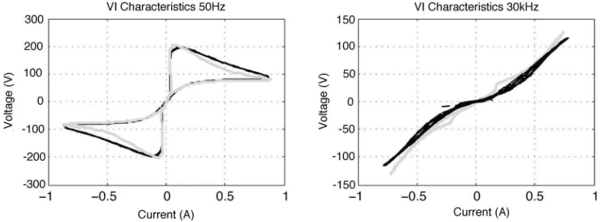
ψion =eE /k Te (3)
whereEis the ionization energy of mercury (10.43 eV). Using (3), it was possible to produce a model that could accurately model either the low- or high-frequency operation but not both. Fig. 1 shows how the relationship between the ionization rate and the electron temperature changes at low and high frequen-cies. This clearly indicates that the ionization rate is not depen-dent upon the electron temperature alone. A second relationship describing ionization rate in terms of electron temperature and electron density was devised. Using the new relationship given in (4), it is possible to get a reasonable approximation to the ionization rate over a wide range of frequencies.
ψion =eb1Te(ne
b2)/b3
. (4)
HOLLOWAYet al.: PHYSICALLY BASED FLUORESCENT LAMP MODEL FOR A SPICE OR A SIMULINK ENVIRONMENT 2103
Fig. 1. Ionization rates for a T8 1.2 m fluorescent lamp, SCCR model (grey) and SPICE-compatible (black) at 50 Hz and 30 kHz.
than (3). Evidence suggests that theV–Iprediction of the model are not very sensitive to the difference in shape between (4) and the SCCR model. The values for b1,b2, and b3 are 0.00042,
0.48633, and7.45×108, respectively. The values were found
using a genetic algorithm that used data from the SCCR model to find the optimum values for the fit.
C. Recombination Rate
The recombination rate is the rate at which electrons and ions move to the wall where they recombine with each other, as this is the dominant recombination method within lamps. It is widely accepted that the electrons and ions move to the wall under ambipolar diffusion, where an electric field is set up to retard the movement of the otherwise fast moving electrons to balance their speed with the heavier mercury ions.
Making the usual assumption [16] that the electron density follows a zeroth-order Bessel function, the recombination rate is given by (5), whereDais the ambipolar diffusion coefficient
given by (6) andRis the lamp radius.
ψrecombination=
2.405 R
2
Da (5)
Da =
µeDi+µiDe
µe+µi
. (6)
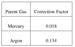
Making the assumption that the heavy particles are in LTE, we can use the Einstein relationship to calculate the ion diffusion coefficient (7). The ion mobility in a mercury–argon gas mixture is found using Blanc’s law (8), whereχHgandχArare correction
factors given in Table I taken from [17], and the gas temperature is assumed to be 45◦higher than the wall temperature.
Di=
kTgasµi
e (7)
µi=Tgas8.069×100.5
P
Hg
χHg
+PAr
χAr
−1
. (8)
TABLE I
CORRECTIONFACTORS FORIONMOBILITY IN AMERCURY–ARGONMIX
The mercury pressure used in (8) is calculated using the em-pirical formula (9) from [18].
ln(1000PHg) = 30.804−0.8254ln(Twall)−7564
Twall.
(9)
The model assumes that the wall temperature is the same as the cold spot temperature. The equation for the electron dif-fusion coefficientDe uses a relationship between the electron
temperature found from the SCCR model.
De=Te4.5×10−7 +Te×102−Te0.0087 + 200. (10)
D. Electron Mobility
Our investigations have indicated that the characteristic “S” shape seen in the V–I characteristics of fluorescent lamps is the result of the changing electron mobility rather than any significant changes in electron density. At frequencies, below a few hundred hertz, it is the change in electron density that dominates the shape of theV–Icharacteristic.
Making the same assumption as in (7) that the electrons are in LTE with each other it is possible to use the Einstein relation to calculate the mobility,µe(11).
µe = eDe
kTeh f
. (11)
The electron diffusion coefficientDehas already been
calcu-lated in (10). As the electron mobility is instrumental in defining the high frequencyV–Icharacteristic but less important at low frequencies, a better approximation to the electron tempera-ture at high frequency has been used instead of the electron temperature that has been used for the rest of the calculations (2), this has been named Teh f. This gives a much better fit
for the high-frequency behavior while not affecting the low-frequency behavior in any appreciable manner. A satisfactory fit with the results from the SCCR model could be obtained using six terms,c1 = 10,c2 = 80,c3 = 2500,c4= 4000,c5 = 8000,
andc6 = 12 000.
Teh f = 2500
n
i= 0
e(−bi/V2) + 4000. (12)
E. Lamp Conductivity
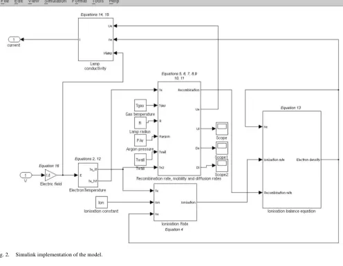
Fig. 2. Simulink implementation of the model.
balance equation:
ne=
ψionization −ψrecombination. (13)
The electron mobility has already been calculated in (11). The current density is calculated by
J =eneµeE. (14)
The lamp geometry is accounted for by
Ilam p=J
2.405
R 2
2πR2 (15)
Vlam p =E×lamp length. (16)
F. Model Implementation
The model has been implemented in both SPICE and Simulink. The Simulink version, shown in Fig. 2, can be used in conjunction with either SimPowerSystems or the Plexsim power toolboxes. In both cases when using the model, it is only neces-sary to provide information about the tubes length, radius, wall
TABLE II LAMPVARIABLES
HOLLOWAYet al.: PHYSICALLY BASED FLUORESCENT LAMP MODEL FOR A SPICE OR A SIMULINK ENVIRONMENT 2105
Fig. 3. Simulated and experimentalV–Icharacteristics for a T8 1.2 m fluorescent lamp at 50 Hz (top) (grey: experimental; black: simulated).
Using these values should allow a reasonable approximation to theV–Icharacteristics for most lamp types under most drive conditions. If a more accurate fit is needed for a particular lamp or drive condition, it is possible to modify these constants, for example, using a genetic algorithm, as presented by [14], how-ever, it is anticipated that the generic constants presented here would be sufficient for most situations.
As well as calculating the terminal V–I. characteristics of the lamp it also provides some information about the lamp’s internal parameters such as the electron density, mobility and temperature, the recombination and ionization rates, and ion mobility.
III. MODELVALIDATION
The model has been compared with experimental results for a T5, 0.8 m lamp, a T8 1.2 m lamp, and T12 1.2 m and 1.8 m lamp. All the lamps were manufactured by Osram. The model’s validity has been tested over a frequency range from 50 Hz to 50 kHz at various power levels.
A. Resistive Ballast
A resistive ballast was chosen as the primary method of vali-dating the model because it is the simplest method of observing the lamp under identical conditions over the entire frequency range. In practice, a resonant ballast is used at high frequency and an inductor used at low frequency. Using a resistive ballast instead of an inductive one at low frequency has the added ben-efit of allowing the observation of the reignition of the lamp that occurs at low frequencies.
The experimental setup used consisted of a laboratory MOSFET power amplifier that drives a mains toroidal step-up transformer to provide the high voltage needed to strike and run the lamp. A 300-Ωnoninductive resistive ballast was placed in series with the lamp to limit the current. The lamp’s electrodes were constantly heated using an isolated flyback converter con-figured to provide a constant power to the electrodes.
1) Lamp Operation at High and Low Frequencies: One area that lamp models for circuit simulation have been deficient in is the ability for the model to work at high and low frequen-cies without adjusting any model parameters. With the switch
to electronic ballasts running at high frequencies the majority of lamp models have focused on the high-frequency operation where the lamp starts to behave as a resistor. This model, being based upon the physical laws governing the lamp’s operation, works equally well for both high and low frequencies.
Fig. 3 shows both the high-frequency and low-frequency op-eration for a T8 1.2 m fluorescent lamp. Good agreement is shown between the experimental and simulated results. The model correctly predicts the magnitude of the reignition spike on the 50 Hz voltage waveforms. The model does not predict the notches that are visible in the 30 kHzV–Icharacteristics. These notches are caused by the onset of oscillations in the plasma, believed to be caused by instabilities at the electrodes, which have not been considered in this model.
2) Lamp Operation at Different Power Levels: Fluorescent lamps exhibit a negative resistance behavior, the larger the cur-rent through the lamp the smaller the voltage across it becomes. Fig. 4 shows the V–I characteristics for a lamp driven at in-creasing lamp powers at 30 kHz. The discrepancy between the experimental results and the simulated results at different power levels is most likely caused by the use of a constant gas temper-ature in the model.
Fig. 4. Experimental (left) and simulated (right)V–Icharacteristics for a T8, 1.2 m fluorescent lamp at 30 kHz running at different power levels.
[image:7.594.77.522.335.695.2]HOLLOWAYet al.: PHYSICALLY BASED FLUORESCENT LAMP MODEL FOR A SPICE OR A SIMULINK ENVIRONMENT 2107
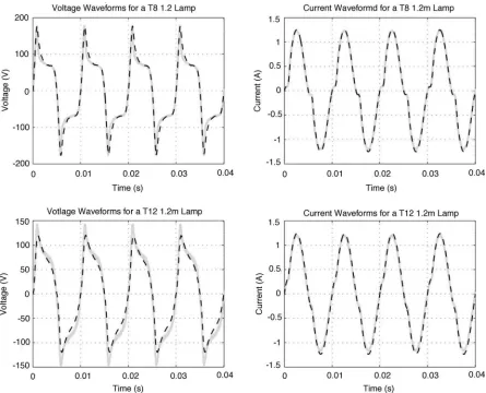
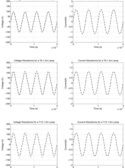
Fig. 6. Voltage and current waveforms for a 1.2 m T8 and T12 lamp and a 0.8 m T5 lamp. Supply voltage of 450 V, 30 kHz (solid lines: experimental; dashed lines: simulated).
is primarily determined by the lamp power and the ambient tem-perature. In practice, under normal operating conditions, a wall temperature of 313 K can be used with acceptable results.
The model shows good agreement for the T5 and T8 flu-orescent lamps, however, it slightly underestimates the
Fig. 7. Voltage and current waveforms for a 1.2 m T8 and T12 lamp with a 1-H inductive ballast (solid lines: experimental; dashed lines: simulated).
model is a reasonably good physical approximation to the lamp.
B. Inductive Ballast
Although the use of magnetic ballasts are gradually being phased out in preference for electronic ballasts, they are still in widespread use and continue to sell in large quantities. This experiment demonstrates the models ability to simulate a flu-orescent lamp that is driven using a magnetic ballast. A 1-H inductor was used for the ballast. The core was suitably large to prevent saturation. The rest of the setup was identical to that presented earlier. The experiment was performed on a T8 1.2 m lamp at 50 Hz with a supply voltage of 350Vpk, this is similar
[image:9.594.319.546.67.168.2]to the conditions in domestic magnetic ballasts in the EU. The model correctly predicts the lamp current (see Fig. 7) but underestimated the magnitude of the reignition spike on the voltage waveform. Once the lamp is reignited, the model is in reasonably close agreement with the experimental results. There is a discrepancy between the accuracy with which the model predicts the lamp’s behavior at low frequency with a resistive ballast, which is generally quite good, and the accuracy achieved with an inductive ballast. The magnitude of the reignition peak is particularly sensitive to small variations in lamp parameters, this results in small errors in the model causing large differences between the predicted and experimental results. Currently, it is
Fig. 8. Resonant ballast driven by a half bridge running from a 100 V supply.
Fig. 9. Before ignition the ballast operates at point A. After ignition the circuitQ-factor is reduced and the lamp operates at point B. To dim the lamp the frequency is increased above resonance to point C.
unclear whether the error is due to an error in the model or the incorrect modeling of the ballast.
C. Example Using a Dimming Resonant Ballast
To demonstrate the model’s ability to handle step changes in frequency and power, a dimming resonant ballast has been constructed. The ballast consists of an inductor in series with a parallel combination of the lamp and a capacitor (see Fig. 8). A dc-blocking capacitor has been incorporated to allow the ballast to run from a unipolar supply. The ballast is driven using a half-bridge arrangement. Before the lamp is lit, the circuit has a very highQ-factor that generates a voltage large enough to strike the lamp, once the lamp is lit theQ-factor drops considerably (Fig. 9). Dimming is achieved by increasing the frequency above resonance. The primary aim of this experiment is to investigate the model’s ability to handle a step change in frequency causing a step change in the lamp power.
The frequency was changed from the resonant frequency of 90–110 kHz resulting in approximately 50% dimming.
[image:9.594.308.555.206.348.2]HOLLOWAYet al.: PHYSICALLY BASED FLUORESCENT LAMP MODEL FOR A SPICE OR A SIMULINK ENVIRONMENT 2109
Fig. 10. Voltage and current waveforms for both experimental (top) and simulated (bottom) step change in frequency from 90 to 110 kHz. This represents a change from 100% lamp power to 50%.
IV. CONCLUSION
A model for a fluorescent lamp has been presented that is suitable for use in circuit design. The model uses physical laws, where possible, and resorts to approximations found from an SCCR model where the solution requires iterations to solve it, for example, the electron temperature.
The model can be used to model any low-pressure mercury-buffer gas fluorescent lamps by entering key lamp parameters, length, radius, cold-spot temperature, and buffer gas fill pres-sure. If fill pressure is not known, a default value dependent on lamp radius is used.
The model has been shown to provide good agreement with experimental results for both low (50 Hz) and high (tens of kilohertzs) frequencies at a wide range of lamp power levels. It has also been shown that it is possible to model a wide range of fluorescent lamp types by providing only key lamp parameters. The model is suitable for modeling both inductive ballasts and resonant ballasts. The model’s ability to handle step changes in frequency and power has also been demonstrated with an example of a dimming resonant ballast.
REFERENCES
[1] Light’s Labour’s Lost, Policies for Energy-Efficient Lighting. Paris, France: OECD, 2006.
[2] V. Francis,Fundamentals of Discharge Tube Circuits. London, U.K.: Methuen & Co. Ltd., 1948.
[3] S. C. Peck and D. E. Spencer, “A differential equation for the fluorescent lamp,” IES Trans., vol. 63, pp. 157–166, Apr. 1968.
[4] P. Horn and U. Mader, “A dynamic model for the electrical character-istics of fluorescent lamps,” inProc. Conf. Rec. IEEE Ind. Appl. Soc. Annu. Meeting, Houston, TX, Oct. 1992, vol. 2, pp. 1928–1934, Cat. No. 92CH31468.
[5] N. Onishi, T. Shiomi, A. Okude, and T. Yamauchi, “A fluorescent lamp model for high frequency wide range dimming electronic ballast simu-lation,” inProc. 14th Annu. Appl. Power Electron. Conf. Expo. (APEC 1999), vol. 2, pp. 1001–1005, Cat. No. 99CH36285.
[6] M. Sun and B. L. Hesterman, “Pspice high-frequency dynamic fluorescent lamp model,” IEEE Trans. Power Electron., vol. 13, no. 2, pp. 261–272, Mar. 1998.
[7] T. Liu, K. Tseng, and D. Vilathgamuwa, “Pspice model for the electrical characteristics of fluorescent lamps,” in Proc. 1998 IEEE 29th Annu. Power Electron. Spec. Conf. (PESC) Rec., Pt. 2,Fukuoka, Japan, 18–21 May. Piscataway, NJ: IEEE, pp. 1749–1754.
[8] M. Ponce, J. Arau, and J. Alonso, “Simple PSPICE high-frequency dy-namic model for discharge lamps,” in Proc. 7th IEEE Workshop Com-put. Power Electron.,Blacksburg,VA, Jul. 16–18, 2000. Piscataway, NJ: IEEE, pp. 293–297.
[9] S. Ben-Yaakov, M. Shvartsas, and S. Glozman, “Statics and dynamics of fluorescent lamps operating at high frequency: Modeling and simulation,”
IEEE Trans. Ind. Appl., vol. 38, no. 6, pp. 1486–1492, Nov./Dec. 2002. [10] G. W. Chang and Y. J. Liu, “A new approach for modeling voltage-current
characteristics of fluorescent lamps,” IEEE Trans. Power Del., vol. 23, no. 3, pp. 1682–1684, Jul. 2008.
[11] K. H. Loo, G. J. Moss, R. C. Tozer, D. A. Stone, M. Jinno, and R. Devonshire, “A dynamic collisional-radiative model of a low-pressure mercury–argon discharge lamp: A physical approach to modeling fluores-cent lamps for circuit simulations,”IEEE Trans. Power Electron., vol. 19, no. 4, pp. 1117–1129, Jul. 2004.
[12] G. Zissis and D. Buso, “Using full physical model for fluorescent lamps in ballast engineering,” in Proc. IEEE Ind. Appl. Soc. (IAS) Conf. Rec., vol. 1, 2003 IEEE 38th IAS Annu. Meeting: Crossroads Innovation,Salt Lake City, UT, Oct. 12–16. Piscataway, NJ: IEEE, pp. 537–541. [13] K. H. Loo, D. A. Stone, R. C. Tozer, and R. Devonshire, “A dynamic
conductance model of fluorescent lamp for electronic ballast design simu-lation,”IEEE Trans. Power Electron., vol. 20, no. 5, pp. 1178–1185, Sep. 2005.
[14] S. Wei, Y. Tam, and E. Hui, “A semi-theoretical fluorescent lamp model for time-domain transient and steady-state simulations,” IEEE Trans. Power Electron., vol. 22, no. 6, pp. 2106–2115, Nov. 2007.
[16] M. A. Cayles, “Theory of the positive column in mercury rare-gas dis-charges,”Brit. J. Appl. Phys, vol. 14, pp. 863–869, 1963.
[17] G. Lister and S. Coe, “Glomac: A one dimensional numerical model for steady state low pressure mercury-noble gas discharges,” Comput. Phys. Commun., vol. 75, no. 1–2, pp. 160–184, 1993.
[18] S. Dushman,Scientific Foundation of Vacuum Technique. New York: Wiley, 1949.
Arran J. Hollowayrecieved the M. Eng. degree in electronic engineering in 2005 from the University of Sheffield, Sheffield, U.K., where he is working toward the Ph.D. in the modeling of low-pressure mercury–argon lamps, with a particular emphasis on models suitable for ballast simulation.
Richard C. Tozer (M’83–SM’98) received the B.Eng. and Ph.D. (CCD device applications) degrees from the University of Sheffield, Sheffield, U.K., in 1970 and 1975, respectively.
After completing the Ph.D. degree, he became a Lecturer at the University of Essex, Colchester, U.K., where he was engaged in active sound cancellation. Since 1980, he has been a Lecturer with the Univer-sity of Sheffield, where he is currently involved in teaching analog circuit design. His current research interests include the application of analog circuits to a wide range of experimental and instrumental problems and is currently centerd around amplitude probability distribution (APD) noise measurement and novel excitation modes for fluorescent lamps.
Dr. Tozer is a Chartered Engineer and a member of the IEE.
Dave A. Stonegraduated in B.Eng. in electronic en-gineering from the University of Sheffield, Sheffield, U.K., in 1984, and the Ph.D. degree from the Univer-sity of Liverpool, Liverpool, U.K., in 1989.