COMPONENTS
WALTER BERGWEILER, N ´URIA FAGELLA, AND LASSE REMPE-GILLEN
Abstract. We show that an invariant Fatou component of a hyperbolic
transcenden-tal entire function is a Jordan domain (in fact, a quasidisc) if and only if it contains only finitely many critical points and no asymptotic curves. We use this theorem to prove criteria for the boundedness of Fatou components and local connectivity of Julia sets for hyperbolic entire functions, and give examples that demonstrate that our re-sults are optimal. A particularly strong dichotomy is obtained in the case of a function with precisely two critical values.
1. Introduction
Dynamical systems that arehyperbolic(or “Axiom A” in Smale’s terminology) exhibit, in a certain sense, the simplest possible behaviour. (For the formal definition of hyper-bolicity in our context, see Definition 1.1 below.) In any given setting, understanding hyperbolic systems is the first step on the way to studying more general types of be-haviour. Furthermore, in many one-dimensional situations, hyperbolic dynamics is either known or believed to be topologically generic (see e.g. [Lyu97, G´S97, KSvS07, RvS15]), and hence many systems are indeed hyperbolic.
In the iteration of complex polynomials p: C→ C, the dynamics of hyperbolic func-tions has been essentially completely understood since the seminal work of Douady, Hubbard and Thurston in the 1980s. In particular, these can be classified – in a va-riety of ways – using finite combinatorial objects such as “Hubbard trees”. Typically, any qualitative question about the iterative behaviour of the map in question can be answered from this encoding.
In addition to polynomial and rational iteration, the dynamical study of transcen-dental entire functions (i.e.non-polynomial holomorphic self-maps of the complex plane) is currently receiving increased interest, partly due to intriguing connections with deep aspects of the polynomial theory. (We refer to the introduction of [RRRS11] for a short discussion.) However, until recently there were only a small number of specific cases where hyperbolic behaviour had been understood in detail (cf. [AO93, BD00b, SZ03] and [Rem06, Corollary 9.3]).
Indeed, it turns out that, even restricted to the hyperbolic case, entire functions can be incredibly diverse: for example, while for many such maps, the Julia sets are known to contain curves along which the iterates tend to infinity, there are also (hyperbolic)
Date May 21, 2015.
2010Mathematics Subject Classification. Primary 37F10; Secondary 30D05, 37F15.
The second author was supported by Polish NCN grant decision DEC-2012/06/M/ST1/00168 as well as grants 2009SGR-792 and MTM2011-26995-C02-02. The third author was supported by a Philip Leverhulme Prize.
1
examples where this is not the case [RRRS11]. Similarly, for some hyperbolic maps there are natural conformal measures in the sense of Sullivan, with associated invariant mea-sures [MU08], while for others such meamea-sures cannot exist [Rem13]. Nonetheless, it was proved recently [Rem09, Theorems 1.4 and 5.2] that, in any given family of entire func-tions, the behaviour of hyperbolic functions can essentially be described completely, in terms of a certain topological model (which however depends on the family in question). A disadvantage of this description is that it is not very explicit. To explain what we mean by this, and to introduce the main question treated in our article, we first provide some of the definitions that were deferred above. A points∈Cis called asingularity of the inverse function f−1 if s is either acritical value (the image of a critical point) or a
finite asymptotic value. The latter means that there is a pathγ to infinity whose image ends at s; the curve γ is then called an asymptotic curve. The set of such singularities is denoted by sing(f−1). Then we call
(1.1) B:={f: C→C transcendental entire : sing(f−1) is bounded}
the Eremenko-Lyubich class (compare [EL92]).
1.1. Definition (Hyperbolicity).
A transcendental entire functionf: C→Cis called hyperboliciff ∈ Band furthermore every element of S(f) := sing(f−1)belongs to the basin of some attracting periodic cycle
of f.
Equivalently, f is hyperbolic if and only if thepostsingular set
P(f) := [
j≥0
fj(sing(f−1))
is a compact subset of the Fatou set (see Proposition 2.1). Recall that the Fatou set, F(f), consists of those points whose behaviour under iteration is stable; more precisely, it contains exactly those points where the family of iterates (fn)
n≥0 is equicontinuous
with respect to the spherical metric. The complement J(f) = C\F(f) is called the Julia set; here the dynamics is unstable.
If a hyperbolic entire function f has an asymptotic value, then it follows immedi-ately that some (but not necessarily all) connected components of F(f) are unbounded, see Figures 1(a) and 1(b). On the other hand, there are also examples where all Fa-tou components appear to be bounded Jordan domains; compare Figures 2(c) and 2(d). Unfortunately, the above-mentioned description from [Rem09] does not allow us to deter-mine when this is the case, and hence the problem remained open even for rather simple explicit cases such as thecosine family, see below. The following result gives a complete answer to this question, and hence provides another step towards the understanding of hyperbolic transcendental entire dynamics.
1.2. Theorem (Bounded Fatou components).
Let f ∈ B be hyperbolic. Then the following are equivalent:
(1) every component of F(f) is bounded;
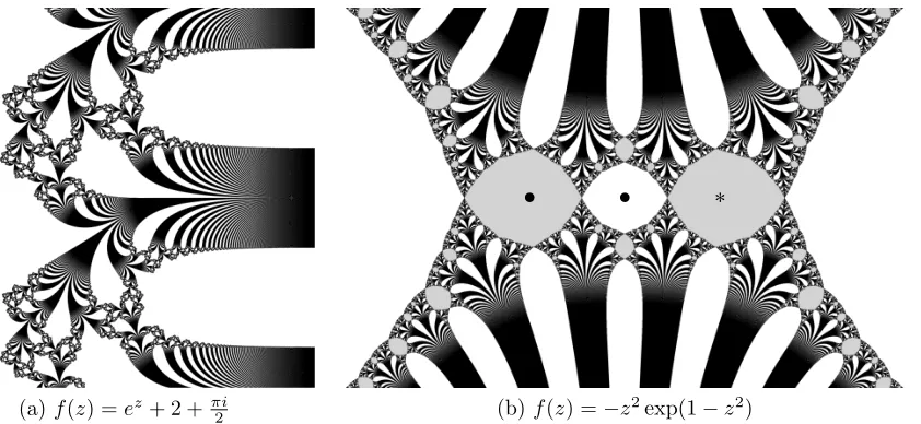
(a)f(z) =ez+ 2 + πi
2 (b)f(z) =−z
[image:3.612.113.534.87.281.2]2exp(1−z2)
Figure 1. Two entire functions with asymptotic values and unbounded Fatou components (the Julia set is drawn in black; Fatou components are in grey and white). On the left is an exponential map; the Fatou set consists of the basin of an attracting orbit of period 3. Every Fatou component U is unbounded and∂U is not locally connected. On the right is a function that plays a crucial role in our construction of Example 1.6. Here there are superattracting fixed points at 0 and −1 (marked with filled circles), and 0 is an asymptotic value. The basin of 0 is coloured white and the basin of −1 is coloured grey – every Fatou component is a Jordan domain, but all pre-periodic components of the basin of 0 are unbounded, and the Julia set is not locally connected. Here and in subsequent images, non-periodic critical points (in this case, the point 1) are marked by asterisks.
Remark. If either (and hence both) of these conditions are true, then in fact all Fatou components are bounded quasidiscs, see Corollary 1.11. (Aquasidiscis a Jordan domain that is the image of the open unit disc under some quasiconformal homeomorphism of the Riemann sphere.)
Condition (2) of Theorem 1.2 can usually be verified in a straightforward manner for specific hyperbolic functions. This is especially easy when sing(f−1) is finite, f
has no asymptotic values and we know that every Fatou component contains at most one critical value (for example, because different critical values converge to different attracting periodic orbits). We shall see (in Proposition 2.9 (1)) that in this case every component ofF(f) contains at most one critical point, and hence we obtain the following corollary:
1.3. Corollary (One critical value per component).
Let f be a hyperbolic entire function without asymptotic values. If every component of
F(f) contains at most one critical value, then every component of F(f) is bounded.
(a)F(f) connected (b) Unbounded components
[image:4.612.85.532.87.415.2](c) Locally connected Julia set (d) Another locally connected Julia set
Figure 2. Julia sets (in dark grey) of some maps in the cosine family, z 7→
acos(z) +b, illustrating Theorem 1.4 and Corollary 1.9.1 (Note that these can easily be reparametrised as z7→sin(a0z+b0) for suitable choices of a0, b0.) The two maps in the top row have unbounded Fatou components and their Julia sets are not locally connected. The maps on the bottom line both have locally connected Julia sets.
map z 7→ λez. This family has been thoroughly studied since the 1980s; compare e.g.
[BR84, Dev84, EL92, RS09] and the references therein. Since exponential maps have an asymptotic value at 0 and no other singular values, in the hyperbolic case there are only unbounded Fatou components (see Figure 1(a)).
Cases where # sing(f−1) = 2 include for instance the cosine (or sine) maps z 7→
sin(az+b), where a, b∈C, a6= 0, with critical values at ±1 but no asymptotic values,
1The maps in Subfigures (a), (c) and (d) have −a = b = λ, with λ = 3/4, λ = 4π/3 and λ = 2,
as well as the family z 7→ azez +b with one critical and one asymptotic value, among
many others (compare [Den13, Fag95]). However, the class of entire maps with two inverse function singularities is far more general than suggested by these simple examples. Indeed, there exist uncountably many essentially different families of entire functions with no asymptotic values and exactly two critical values; the same is true for functions with two asymptotic values, or one critical and one asymptotic value. By this we mean that there exists an uncountable collection F of functions of this type, such that none of the functions in F can be obtained from another by pre- and post-composition with plane homeomorphisms. (The existence of such a collection follows from the classical theory of line complexes; compare [GO08, Chapter 7] and also Observation 5.2 below.)
Drasin [Dra07] and Merenkov [Mer08] have constructed maps of this class that have irregular and arbitrarily fast growth, respectively. More recently, Bishop [Bis15] has described a method for constructing functions with no asymptotic values, two critical values and only simple critical points, having essentially arbitrary prescribed behaviour near infinity. These functions can have dynamical properties that are very different from those of the simple examples mentioned above. For example, Bishop shows [Bis15, Section 18] that the above-mentioned example from [RRRS11, Theorem 1.1], where the
escaping set
I(f) :={z ∈C: fn(z)→ ∞}
contains no unbounded continuous curves, can be realised within this class.
Theorem 1.2 allows us to formulate a striking dichotomy when # sing(f−1) = 2:
1.4. Theorem (Dichotomy for functions with two critical values).
Let f: C →C be a transcendental entire function without finite asymptotic values and exactly two critical values. Assume furthermore that f is hyperbolic, i.e. both critical values tend to attracting periodic orbits of f under iteration. Then either
(1) every connected component U of F(f) is unbounded, and ∂U is not locally con-nected at any finite point, or
(2) every connected component of F(f) is a bounded quasidisc.
In case (1), all critical points of f belong to a single periodic Fatou component.
Here “local connectivity” of a set K at a point z means that there are arbitrarily small connected neighbourhoods of z in K; we do not require these neighbourhoods to be open. (Sometimes this property is instead referred to as “connected im kleinen”; compare e.g. [Rem08].) Of course, the boundary of a quasidisc is locally connected at every point. Hence, for hyperbolic maps with two critical values, there are two extremely contrasting possibilities for the shape of all Fatou components.
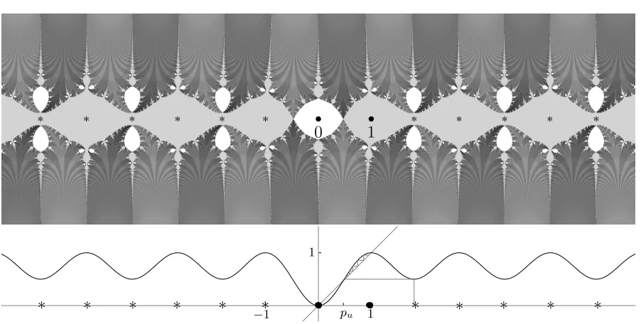
0 1
1
pu −1
1
* * * * *
[image:6.612.82.533.71.299.2]* * * * * *
Figure 3. The function from Example 1.5 (shown here for u= 3) has three critical values and two fixed Fatou components, one of which is a bounded Jor-dan domain, while the other is unbounded with non-locally-connected bound-ary. The fixed points 0 and 1 are superattracting; the basin of 0 is depicted in white, the basin of 1 in light grey, and the Julia set in darker tones of grey. Non-periodic critical points are marked by asterisks.
even without the assumption of hyperbolicity; it is conjectured there that this also holds whenever |a| ≥1.
Without further hypotheses, Theorem 1.4 does not hold for larger numbers of critical values, as shown by the following example (see Figure 3).
1.5. Example (Unbounded and bounded Fatou components). Define
f(z) =
u−cos q
arcosh2u+π2
z2−arcosh2u
u+ 1
where u > 1. Then f has no asymptotic values and three critical values 0, 1 and
cu = (u−1)/(u+ 1). The points 0 and 1 are superattracting fixed points and for large
u (in fact, for u >2.7981186. . .) the critical value cu and all positive critical points are contained in the immediate attracting basin of 1. The immediate basin of 0is a bounded quasidisc while the immediate basin of 1 is unbounded and not locally connected at any finite point; see Figure 3.
Even when the periodic Fatou components are Jordan domains, it is possible for some preimage components to be unbounded:
1.6. Example (Unbounded preimages of bounded Fatou components).
There exists an entire function f, with three critical valuesw1, w2, w3 and no asymptotic
(a) w1 and w2 are superattracting fixed points with immediate basins bounded by a
Jordan curve;
(b) w3 is contained in the immediate basin of w1;
(c) the preimage of the immediate basin of w1 has an unbounded component.
Local connectivity of Julia sets. A key question in polynomial dynamics is whether a given Julia set islocally connected. This is known to hold for large classes of examples, including all hyperbolic maps, and implies a complete description of the topological dynamics of the map in question (compare [Dou93]).
Local connectivity of Julia sets of transcendental entire functions has also been stud-ied by a number of authors (see e.g. [Mor99, BM02, Osb13]). This problem is closely connected to the boundedness of Fatou components, mentioned above. Indeed, if any component of F(f) is unbounded, then J(f) cannot be locally connected (compare [BD00a, Theorem E] and Lemma 2.4 below); in particular, hyperbolic functions with asymptotic values do not have locally connected Julia sets. We may ask whether the conditions in Theorem 1.2, which describe precisely when all Fatou components are bounded, also ensure local connectivity of the Julia set. It turns out that this is not the case:
1.7. Example (Non-locally connected Julia set).
There exists an entire function f, having two critical values 0 and 1 and no other sin-gularities of the inverse function, such that the following hold:
(a) 0 and 1 are superattracting fixed points;
(b) every Fatou component of f is bounded by a Jordan curve;
(c) the Julia set of f is not locally connected.
The basic idea behind the construction is to use critical points of extremely high degree to simulate the behaviour of an asymptotic value and create (pre-periodic) Fatou components of large diameter; compare Figure 5 in Section 5. This suggests that, to ensure local connectivity, we should require a bound on the multiplicities of critical points within any one Fatou component. Indeed, using a result of Morosawa (see Theorem 2.5 below), we obtain the following consequence of Theorem 1.2.
1.8. Corollary (Bounded degree implies local connectivity).
Letf ∈ Bbe hyperbolic with no asymptotic values. Suppose that there is a numberN such that every component of F(f) contains at most N critical points, counting multiplicity. Then J(f) is locally connected.
Again, the additional assumption becomes particularly simple when every Fatou com-ponent contains at most one critical value, or when # sing(f−1) = 2.
1.9. Corollary (Locally connected Julia sets).
Let f be a hyperbolic function without asymptotic values. Suppose that
(a) every component of F(f) contains at most one critical value, or
(b) # sing(f−1) = 2 and every component of F(f) is bounded.
One interesting consequence of the preceding discussion is that, in the transcendental setting,local connectivity does not imply simple topological dynamics. Indeed, the exam-ples of Bishop that were mentioned above have only critical points of degree at most 4 and, by precomposing such an example with a linear map, we can ensure that both criti-cal values are superattracting fixed points. Hence Corollary 1.9 applies to these families and therefore the Julia set is locally connected. On the other hand, by the results of [Rem09], the “pathological” behaviour near infinity is preserved by such a composition. In particular, we can find hyperbolic entire functions with locally connected Julia sets where the escaping set does not contain any curves to ∞, or even (using recent results from [Rem14]) such examples where the Julia set contains an uncountable collection of pairwise disjoint and dynamically natural pseudo-arcs. (The pseudo-arc is a certain hereditarily indecomposable continuum; cf. [Nad92, Exercise 1.23].)
Boundedness of immediate basins. The key step in establishing Theorem 1.2 is to verify that all periodic Fatou components of the map f are bounded, provided that condition (2) in the theorem holds. This is achieved by the following result, which gives a variety of conditions equivalent to the boundedness of a Fatou component.
1.10. Theorem (Immediate basins of hyperbolic maps).
Let f ∈ B be a hyperbolic transcendental entire function, and let D be a periodic Fatou component of f, say of period p≥1. Then the following are equivalent:
(a) D is a quasidisc;
(b) D is a Jordan domain;
(c) Cb \D is locally connected at some finite point of ∂D; (d) D is bounded;
(e) D does not contain a curve to infinity;
(f) the orbit ofDcontains no asymptotic curves and only finitely many critical points;
(g) fp:D→D is a proper map;
(h) for at least two distinct choices of z ∈D, the set f−p(z)∩D is finite.
As mentioned, the key new implication here is (f)⇒(d); the remaining equivalences and implications can be obtained by well-established methods, although some of them appear to be folklore. This part of the proof relies on a result from [Rem09], which states that hyperbolic maps are uniformly expanding on a suitable neighbourhood of their Julia sets; see Proposition 2.2 below, and compare also [RS99, Theorem C].
We remark that the conclusion of the theorem does not hold if we omit the requirement that f ∈ B from the definition of hyperbolicity. Indeed, consider f(z) := ez +z + 1, which is precisely Newton’s method for finding roots of z 7→e−z+ 1. Then the singular values of f are precisely the infinitely many superattracting cycles ak = (2k + 1)πi
(with k ∈ Z), and f has degree two when restricted to the invariant Fatou component containing ak. However, all these components are unbounded.
As a consequence of Theorem 1.10, we obtain the result announced after Theorem 1.2, concerning quasidiscs:
1.11. Corollary (Bounded components are quasidiscs).
Remark 1. It is possible for pre-periodic unbounded Fatou components to be quasidiscs; indeed this is the case for two of the components in Figure 1(b).
Remark 2. This Corollary can also be deduced directly from known results and methods. Indeed, a theorem of Morosawa [Mor99, Theorem 1] implies that every bounded Fatou component of a hyperbolic function is a Jordan domain. It is not difficult to deduce that the boundary must in fact be a quasicircle.
Bounded Fatou components and local connectivity beyond the hyperbolic setting. In this article, we consider only hyperbolic functions, and use uniform expan-sion estimates to establish our results. There are a number of weaker hypotheses that will also suffice; here we mention only that all our proofs go through for entire functions without asymptotic values that are strongly subhyperbolic in the sense of Mihaljevi´ c-Brandt [MB12]. The theorems on Jordan Fatou components should extend even more generally, e.g. assuming that the function is geometrically finite in the sense of [MB10], and there are no asymptotic values on the boundaries of Fatou components. (However, in the presence of parabolic points the boundaries will no longer be quasicircles.) In view of the recent result of Roesch and Yin [RY08] that all bounded attracting (and parabolic) Fatou components of polynomials are Jordan domains, it is plausible that the same always holds also in the entire transcendental setting, without additional dynamical assumptions on the function f:
1.12. Conjecture.
Let f be a transcendental entire function, and let D be an immediate attracting or parabolic basin. If D is bounded, then D is a Jordan domain.
Structure of the article. In Section 2, we shall collect the prerequisites required to prove our theorems. The proof of Theorem 1.10 relies crucially on a uniform expansion estimate (Proposition 2.2) for hyperbolic entire functions, but we shall require a number of additional results to deduce our theorems as stated. To keep the article self-contained, to emphasise the elementary nature of our arguments, and to provide a convenient reference for future studies of hyperbolic functions, we provide proofs or sketches of proofs where appropriate. We do use results of Heins [Hei57] and Baker-Weinreich [BW91] without further comments on their proofs. However, we emphasise that these are required only to state properties (c) and (h) of Theorem 1.10 in as weak a form as possible, rather than being essential to the remainder of the proof.
In Section 3, we prove our main result, Theorem 1.10, and deduce the remaining theorems stated in the introduction in Section 4. Finally, Section 5 is dedicated to the construction of Examples 1.5, 1.6 and 1.7, using a method of MacLane and Vinberg.
2. Preliminaries
Notation. As usual, we denote the complex plane byC, and the Riemann sphere byCb. Throughout the article,f will denote a transcendental entire function, usually belonging to the Eremenko-Lyubich class B as defined in (1.1). Recall from the introduction that S(f) := sing(f−1) denotes the set of singular values of f.
If A, B ⊂ C, the notation A b B (“A is compactly contained in B”) will mean that A is bounded and A⊂B. The interior of a set A⊂C is denoted by int(A).
We refer to [Ber93] for background on transcendental iteration theory, and to [BM07] for background on hyperbolic geometry.
Hyperbolicity and uniform expansion. Hyperbolicity is a key assumption in our results. We recall here some important properties. While these are well-known, we are not aware of a suitable reference, and hence provide a detailed proof here for the reader’s convenience.
2.1. Proposition (Hyperbolic functions).
Let f : C → C be a transcendental entire function. Then f is hyperbolic if and only if P(f)bF(f).
If f is hyperbolic, thenF(f)is a finite union of attracting basins, and every connected component of F(f) is simply-connected. Furthermore, there is a compact set K ⊂F(f)
such that f(K) ⊂ int(K) and S(f) ⊂ int(K). The set K can be chosen as the closure of a finite union of pairwise disjoint Jordan domains with analytic boundaries, no two of which belong to the same Fatou component.
Proof. First suppose thatf is hyperbolic. To see thatf has only finitely many attracting basins note that S(f) is compact, and that the Fatou components of f form an open covering of S(f) by assumption. Hence only finitely many Fatou components intersect S(f). On the other hand, every periodic cycle of attracting Fatou components contains at least one singular value by Fatou’s Theorem [Ber93, Theorem 7], so we see that the number of such cycles is finite. It follows, in particular, that the postsingular set P(f) is compact and contained in the Fatou set.
that intersect P(f), we see that
K := [
U∩P(f)6=∅
D(U)
has the required properties.
From now on, assume only thatP(f)bF(f), and letU be a component ofF(f). Then U cannot be a Siegel disc, since otherwise we would have∂U ⊂ P(f) [Ber93, Theorem 7], and hence P(f)∩J(f) 6= ∅, which contradicts our assumption. This implies that all limit functions of the family{fn|
U: n∈N} are constant, possibly infinite. Sincef ∈ B,
we cannot have fn|
U → ∞, by a result of Eremenko and Lyubich [EL92, Theorem 1].
Hence there exists a subsequence of (fn|
U) which tends to a finite constant a ∈ C.
A result of Baker [Bak70, Theorem 2] implies that a∈ P(f). By assumption, it follows that a∈F(f). This implies that U can be neither a parabolic nor a wandering domain. It follows that a must in fact be an attracting periodic point, andU is a component of its attracting basin. Hence F(f) consists of only of attracting basins. In particular, f
is hyperbolic, and the proof is complete.
We remark that Bishop [Bis15] recently proved that the class B contains non-hyper-bolic functions that do have wandering domains. (The orbits of these domains accumu-late both at ∞ and at some finite points. Wandering domains with the latter property had been constructed earlier by Eremenko and Lyubich [EL87, Example 1], but in their examples it was not clear whether the function could be taken to be in B.)
The key element in our proof of Theorem 1.10 will be the fact that hyperbolic functions are uniformly expanding, with respect to a suitable conformal metric.
2.2. Proposition (Uniform expansion for hyperbolic functions [Rem09, Lemma 5.1]). Let f: C →C be a hyperbolic transcendental entire function, and let K be the compact set from Proposition 2.1. That is, f(K)⊂int(K) and S(f)⊂K.
Define W :=C\K and V :=f−1(W). Then there is a constant λ >1 such that
kDf(z)kW ≥λ
for all z ∈ V, where kDfkW denotes the derivative of f with respect to the hyperbolic metric of W.
Idea of the proof. For completeness, let us briefly sketch the proof of this fact; we refer to [Rem09] for details. Since f: V →W is a covering map and V ⊂W, we have
kDf(z)kW =
ρV(z)
ρW(z)
>1
for all z ∈V. It follows that it suffices to prove
ρW(z) = o(ρV(z))
as z → ∞. By standard estimates, we have
ρW(z) =O
1
|z|log|z|
while for V it is shown in [Rem09] that
1 ρV(z)
=O(|z|).
(This uses the fact thatC\V =f−1(K) contains a sequence (wn) with |wn+1| ≤C|wn|,
for a constant C > 1, together with estimates on the hyperbolic metric in a
multiply-connected domain.) This completes the proof.
Local connectivity. We shall use the following characterization of local connectivity for compact subsets of the Riemann sphere.
2.3. Lemma (LC Criterion [Why42, Thm. 4.4, Chapter VI]).
A compact subset of the Riemann sphere is locally connected if and only if the following two conditions are satisfied:
(a) the boundary of each complementary component is locally connected;
(b) for every positive ε there are only finitely many complementary components of spherical diameter greater than ε.
We will apply the result above to study the local connectivity of Julia sets, even though we consider these to be subsets ofC rather than of Cb. However, it is well-known that a continuum cannot fail to be locally connected at a single point [Nad92, Corollary 5.13]. Hence it follows that J(f) is locally connected if and only if J(f)∪ {∞}is.
As mentioned in the introduction, a locally connected Julia set cannot have an un-bounded Fatou component [Osb13, Corollary 1.2].
2.4. Lemma (Local connectivity implies bounded Fatou components).
Let f be an entire transcendental function. If F(f) has an unbounded Fatou component, then J(f) is not locally connected.
Proof. Let U be an unbounded component of F(f). First suppose that there is some iterated preimage component ˜U ofU that is not periodic. It follows that, for any bounded open setDintersecting the Julia set, there are infinitely many different unbounded Fatou components (namely iterated preimages of ˜U) that intersect D. Hence condition (b) of Lemma 2.3 is violated, and J(f) is not locally connected.
If no such component ˜U exists, then U is completely invariant for some iterate fn. It
follows that J(f) =J(fn) is not locally connected by [BD00a, Corollary 3].
The following result shows that, once we know that all immediate attracting basins are Jordan, we can already make conclusions about the local connectivity of the Julia set – provided that there is a bound on the degree off on any pre-periodic Fatou component.
2.5. Theorem (Bounded components and bounded degree imply local connectivity). Letf ∈ Bbe hyperbolic with no asymptotic values. Suppose that every immediate attract-ing basin of f is a Jordan domain. If there is N such that the degree of the restriction of f to any Fatou component is bounded by N, then J(f) is locally connected.
components. Our Examples 1.6 and 1.7 show that this assumption is necessary. A more general statement (which includes the corrected hypotheses) can be found in [BM02, Theorem 4]. For convenience, let us show how the result can be obtained from Proposi-tion 2.2.
Proof of Theorem 2.5. We only need to establish part (b) of Lemma 2.3. By Proposi-tion 2.1, all components of F(f) are simply-connected. Hence, if U and V are Fatou components with f(U)⊂V and V ∩S(f) =∅, then f: U →V is bijective. Since S(f) is compactly contained in the Fatou set, only a finite number k of Fatou components intersect the singular set.
LetU be a pre-periodic Fatou component, say of pre-periodn, and letV =fn(U) be the first periodic Fatou component on the orbit of U. The assumption implies that the degree of fn: U → V is bounded by Nk. Hence – using that V is a Jordan domain –
the boundary ∂U covers ∂V at most Nk times when mapped under fn. Let W and
λ be as in Proposition 2.2. We can cover ∂V by, say, M simply-connected hyperbolic discs (with respect to the hyperbolic metric of W). Since f has only finitely many periodic Fatou components, the numberM is bounded independently ofU. Letrbe the maximal hyperbolic diameter of these discs. Proposition 2.2 implies that we can cover ∂U byNkM hyperbolic disks of diameter r/λn. Thus the hyperbolic diameter of U in
W is bounded by NkM r/λn, which tends to zero exponentially as n tends to infinity.
Furthermore, for a given n, the Fatou components of pre-period n can only accumulate at infinity (by the open mapping theorem), and hence only finitely many of them have spherical diameter greater than a given number ε >0. This establishes property (b) of
Lemma 2.3, and completes the proof.
Remark. Alternatively, we could use distortion principles for maps of bounded degree to see that every Fatou component U contains an open disc of size comparable to the diameter of U. Again, this implies (b) in Lemma 2.3.
In order to state some of our results concerning local connectivity of Fatou component boundaries, we shall use the following theorem, which is due to Baker and Weinreich [BW91]. We remark that this result is not central to our arguments, but rather allows us to state some conclusions (e.g. in Theorem 1.4) more strongly than would otherwise be possible.
2.6. Theorem (Boundaries of periodic Fatou components).
Let f be a transcendental entire function, and suppose that U is an unbounded periodic component of F(f) such that fn|U does not tend to infinity. Then Cb \U is not locally
connected at any finite point of ∂U.
Proof. Baker and Weinreich proved that, under these assumptions, the impression of every prime end of U contains∞. Equivalently, ifϕ: D→U is a conformal map (which exists by the Riemann mapping theorem) and z0 ∈ ∂D, then there exists a sequence zn ∈Dsuch that zn →z0 and ϕ(zn)→ ∞.
in Cb \U. There is a small round disc D around z0 such that the Euclidean length of γ :=ϕ(D∩∂D) is sufficiently short to ensure that both endpoints ofγ are inK, and that K∪γ does not separateϕ(0) from∞. (This follows from a well-known application of the length-area principle – see e.g. [Pom92, Proposition 2.2], which strictly speaking applies only to bounded domains, but whose proof yields the desired result in the unbounded case upon replacing Euclidean length and area with their spherical analogues.) It follows that ϕ(D∩∂D) is contained in the bounded complementary component ofK∪γ, which is a contradiction to the above result by Baker and Weinreich. (Alternatively, we may additionally assume that the prime end corresponding to z0 is symmetric, as the set
of asymmetric prime ends is at most countable [Pom92, Proposition 2.21]. By [CP03, Corollary 1], the corresponding impression is contained in K – a contradiction.)
Finally, we shall require a number of facts concerning the mapping behaviour of entire functions on preimages of simply-connected domains. While these results are certainly not new, we are again not aware of a convenient reference and therefore include the proofs. In our arguments, we shall use the following simple lemma.
2.7. Lemma (Coverings of doubly-connected domains).
Let A, B ⊂ C be domains and let f: B → A be a covering map. Suppose that A is doubly-connected. Then either B is doubly-connected and f is a proper mapping, or B
is simply-connected (and f is a universal cover, of infinite degree).
Proof. The fundamental group ofA is isomorphic to Z. The fundamental group ofB is thus isomorphic to a subgroup of Z. As the only subgroups of Zare the trivial one and
the groups kZ with k≥1, the conclusion follows easily.
2.8. Proposition (Mapping of simply-connected sets).
Let f be an entire function, let D ⊂ C be a simply-connected domain, and let De be a
component of f−1(D). Then either
(a) f: De →D is a proper map (and hence has finite degree), or (b) f−1(w)∩
e
D is infinite for every w∈D, with at most one exception.
In case (b), eitherDe contains an asymptotic curve corresponding to an asymptotic value
in D, or De contains infinitely many critical points.
Proof. A theorem by Heins [Hei57, Theorem 4’] implies that either (b) holds, or the number of preimages of w∈D inDe (counting multiplicity) is finite and constant in D. It is elementary to see that the latter is equivalent to (a).
To prove the final statement, it is sufficient to consider the case where f: De → D has no asymptotic values inD and only finitely many critical values (otherwise, there is nothing to show). This implies that this map is an infinitebranched covering; i.e., every point z0 ∈Dhas a simply-connected neighbourhoodU such that every componentUe of f−1(U)∩D is mapped as a finite covering, branched at most over z
0.
a further point a ∈ D by simple arcs τ1, . . . , τm which do not intersect except in their
common endpoint a. Set T = Sm
j=1τj and Te := f−1(T)∩De. Now D\T is doubly-connected andf: De\Te→D\T is a covering of infinite degree. By Lemma 2.7 this map must be a universal covering, and thus every componentT0 ofTeis unbounded. Sincef is a branched covering map, T0 consists of infinitely many preimages ofT, joined together only at critical points. This proves that De contains infinitely many critical points.
In our applications, the function f will always be hyperbolic, and hence the set of singular values stays away from the boundary of D. In this case, we can say more:
2.9. Proposition (Preimages of sets with non-singular boundary).
Let f, D and De be as in Proposition 2.8, and assume additionally that D∩S(f) is
compact.
(1) If #D∩S(f)≤1, then De contains at most one critical point of f. (2) If S(f)⊂D, then De =f−1(D).
(3) In case(a) of Proposition 2.8, if D is a bounded Jordan domain (resp. quasidisc) such that ∂D∩S(f) = ∅, then De is also a bounded Jordan domain (resp.
qua-sidisc).
(4) In case (b) of Proposition 2.8, the point ∞ is accessible from De.
Proof. Set SD :=S(f)∩D. If #SD = 1, then f: De\f−1(SD)→D\SD is conformally equivalent to an unramified covering of the punctured unit disc. By Lemma 2.7, it follows that De contains at most one critical point. We have proved (1).
Now let U ⊂D be simply-connected such that SD ⊂ U b D. Set Ue :=f−1(U)∩De. By the maximum principle, every component of Ue is simply-connected. We will show that Ue is connected. Indeed, let z, w ∈Ue, and let eγ ⊂De be a smooth arc connecting z and w. Setγ =f(γe). Since SD has a positive distance from∂U, the curve γ contains at
most finitely pieces that connect SD to ∂U. By cutting the curve at one point in each
of these pieces, we may divide it into finitely many segments, some that may intersect S(f) but are contained in U, and some that may leave U but do not intersect S(f). We construct a new curve γ0 ∈U which equals γ in those segments contained in U but is only homotopic to γ in D\S(f), relative to the endpoints, in the remaining pieces. These homotopies can be lifted to De\f−1(S(f)) since f is a covering there, resulting in a curveeγ0 ⊂Ue connecting z andw. HenceUe is connected. In particular, this proves (2) (replacing D byC and U byD).
For the remainder of the proof, let us require additionally thatU is a bounded Jordan domain with U b D. Then A := D\U is doubly-connected. Consider the set Ae := f−1(A)∩
e
D. On every component of Ae, the restriction of f is a holomorphic covering map, since SD ⊂U. By Lemma 2.7, the components of Aeare either doubly- or simply-connected.
disjoint from S(f), then we can apply Proposition 2.8 to a slightly larger Jordan disc D0 without additional singular values, so the restriction of f to the preimage of D0 containing De is still proper. Then, f: ∂De →∂D is a finite degree covering map, which proves that∂De is indeed a Jordan domain. Of course the property of being a quasicircle is preserved under a conformal covering map. This establishes (3).
Now suppose that every component V of Ae is simply-connected. Then f: V → A is a universal covering, and hence has infinite degree. The preimage of any simple non-contractible closed curve inAunder this covering is a Jordan arc inAetending to infinity in both directions, and hence ∞ is accessible from De, proving (4).
Remark 1. In (3), to conclude that ˜D is bounded, it is enough to assume that ∂D has exactly two complementary components, rather than that∂Dis a Jordan curve. Indeed, this follows from the original statement, since we can surround D by a Jordan curve γ such that the Jordan domain W bounded by γ does not contain any singular values other than those already in D. The claim then follows from the Proposition as stated.
Remark 2. In the case when f: De →D is proper but De is unbounded, we do not know whether ∞ is always accessible from De. Indeed, this is an open question even when D =De is an unbounded Siegel disc of an exponential map. Also compare the question in [BD99, p. 439, ll. 8–9].
3. Periodic Fatou components
Proof of Theorem 1.10. Letf ∈ Bbe hyperbolic, and let D be an immediate attracting basin of f, say of period p. By passing to an iterate, we may assume without loss of generality that p= 1. Recall that D is simply-connected (by the maximum principle).
Clearly (a)⇒(b)⇒(c), as any quasidisc is Jordan, and the complement of any Jordan domain is locally connected at every point. On the other hand, if Cb \ D is locally connected at any finite point of ∂D, thenDis bounded by Theorem 2.6. So (c) implies (d).
Clearly, if Dis bounded, then D cannot contain a curve to∞, and hence (d)⇒(e). Since f is hyperbolic, S(f)∩D is compact and we may apply Proposition 2.9 (4) to conclude that, if D does not contain a curve to infinity, then alternative (a) of Propo-sition 2.8 holds. This in turn implies that D contains only finitely many critical points and no asymptotic values, and, again by Proposition 2.8, this is in turn implies that f: D → D is a proper map. Hence (e)⇒(f)⇒(g). Since any proper map has finite degree, we have (g)⇒(h).
It remains to prove (h)⇒(a). So suppose that at least two points in D each have at most finitely many preimages in D. We must show that ∂D is a quasicircle. We shall first prove that ∂D is a bounded curve. In the rational case, this argument goes back to Fatou [Fat20, p. 83]; compare [Ste93, Chapter 5, Section 5], and using the uniform expansion from Proposition 2.2, the proof goes through essentially verbatim.
To provide the details, letU0 bDbe a bounded Jordan domain with analytic
bound-ary such that f(U0)⊂U0 and S(f)∩D⊂U0; such a domain exists by Proposition 2.1.
By Proposition 2.8, f: D → D is a proper map of some degree d ≥ 1. For n ≥ 1, set Un :=f−n(U0)∩D. ThenD=
Now, due to the choice of U0, we see thatfn: D\Un→A :=D\U0 is a finite-degree
covering map (of degree dn) over the doubly-connected domain A. By Lemma 2.7, the domain D\Un is also doubly-connected, and hence Un is connected for all n.
Further-more, by Proposition 2.9 (3), applied to Un and U0, we see that each Un is a Jordan
domain. Hence f: ∂Un+1 →∂Un is topologically ad-fold covering over a circle for every
n ≥0.
We claim that we can find a diffeomorphism
ϕ: W →D\U0, W :={z ∈C: 1/e <|z|<1},
such that
(3.1) f(ϕ(z)) =ϕ(zd) when e−1/d<|z|<1.
Indeed, since f: ∂U1 → ∂U0 is a d-fold covering, we can define ϕ on the circles
{ln|z| =−1} and {ln|z| =−1/d} so that the functional relation (3.1) is satisfied. By interpolation, we extend ϕ to a diffeomorphism
{z ∈C: −1<log|z| <−1/d} →A0 :=U1\U0.
Consider the annuli An :=Un+1\Un. Since each f: An+1 → An is a d-fold covering
map of annuli, we can inductively lift ϕ to a map
z ∈C: −d−n<ln|z|<−d−(n+1) →An,
and our initial choice ofϕensures that this lift can be taken to extend the original map continuously. This completes the construction of ϕ.
Now let ϑ ∈R and n≥0, and consider the curve
γn,ϑ :=ϕ({ea+iϑ: −d−n≤a ≤ −d−(n+1)}).
By the functional relation (3.1), γn,ϑ is the image of the arc γ0,ϑ·dn under some branch of f−n. Recall from Proposition 2.2 that
(3.2) kDf(z)kW ≥λ
whenever z, f(z) ∈/ K, where K is the compact set from Proposition 2.1, W = C\K, and λ >1 is a suitable constant.
Since D\U0 ⊂W, it follows that
`W(γn,ϑ)≤λ−n`W(γ0,ϑ·dn)≤λ−nmax
e
ϑ
`W(γ0,ϑe).
Thus, for n ≥0, the functions
σn: R/Z→D σn(t) =ϕ
e−d−n+2πit∈∂Un
form a Cauchy sequence in the hyperbolic metric of W asn → ∞. Hence there exists a limit functionσn →σwhich is the continuous extension ofϕto the unit circle. It follows
that ∂Dis indeed a continuous closed curve. By the maximum principle, ∂D=∂D and
C\D has no bounded connected components. Hence ∂D is a Jordan curve.
polynomial of degree d with an attracting fixed point whose immediate basin contains all the critical values. Such a basin is completely invariant under the polynomial and its
boundary is a quasicircle; hence ∂D has the same properties.
Remark. Alternatively, to avoid the use of the straightening theorem, it is possible to verify the geometric definition of quasicircles directly. This definition requires that the diameter of any arc of ∂D is comparable to the distance between its endpoints. That condition is trivially satisfied on big scales, and we can transfer it to arbitrarily small scales using univalent iterates. (We thank Mario Bonk for this observation.)
4. Bounded Fatou components and local connectivity of Julia sets
We now deduce the remaining theorems stated in the introduction, using Theo-rem 1.10.
Proof of Corollary 1.11. Let f be hyperbolic. By Theorem 1.10, any bounded periodic
component of F(f) is a quasidisc. Now, if U is any bounded Fatou component, then clearly U contains only finitely many critical points and no asymptotic curves. Hence f: U → f(U) is a proper map by Proposition 2.8, and if f(U) is a quasidisc, then U is also a quasidisc by part (3) of Proposition 2.9. Hence, by induction every bounded
Fatou component of f is a quasidisc, as claimed.
Proof of Theorem 1.2. Letf ∈ Bbe hyperbolic. Iff has no asymptotic values and every Fatou component contains at most finitely many critical points, then every periodic Fatou component is a bounded quasidisc by Theorem 1.10. Moreover, by Proposition 2.8 and part (3) of Proposition 2.9, ifU is any Fatou component off, thenf: U →f(U) is a proper map, and if f(U) is a bounded quasidisc, then so isU. By induction on the pre-period of U, it follows all Fatou components are indeed bounded quasidiscs.
On the other hand, if f has an asymptotic value, this value belongs to the Fatou set by hyperbolicity. Hence f has an unbounded Fatou component. Finally if some Fatou component U contains infinitely many critical points, these can only accumulate
at infinity and therefore U is unbounded.
Proof of Corollary 1.3. Letf be hyperbolic with no asymptotic values, and assume that every Fatou component contains at most one critical value. By Proposition 2.9 (1), it follows that each Fatou component also contains at most one (possibly high-order) critical point. Thus every Fatou component is bounded by Theorem 1.2.
Proof of Theorem 1.4. Suppose thatf is hyperbolic without asymptotic values, and with exactly two critical values. Assume first that both critical values belong to the same Fatou component D. Then D0 := f−1(D) is connected by Proposition 2.9 (2) and
unbounded by the Casorati-Weierstrass theorem. Thus D0 is an unbounded component
of F(f) that contains all critical points of f. By Fatou’s theorem [Ber93, Theorem 7], each cycle of attracting periodic components of F(f) must contain a critical point, and hence D0 is periodic. By Theorem 2.6, ∂D0 is not locally connected at any point.
Moreover, if U is any component of F(f), then, by Proposition 2.1, there exists a minimal number k such that fk(U) = D
0. Since ∞ is accessible from D0 by
locally connected at any finite point, we shall show thatfk maps∂U homeomorphically
to ∂D0. Indeed, let Γ ⊂ D be an arc to infinity that contains both critical values. By
the choice of k, we know that fj(U) is disjoint from D for j = 1, . . . , k, since D has no preimage components apart from D0. Thus there is a branch of f−1 on C\Γ that
maps fk(U) to fk−1(U) homeomorphically, and hence we have established case (1) of
Theorem 1.4.
Assume now that the critical values are not both in the same Fatou component. Then every Fatou component contains at most one of them. By Corollaries 1.3 and 1.11,
case (2) of Theorem 1.4 is satisfied.
Proof of Corollary 1.8. Let f ∈ B be hyperbolic with no asymptotic values, let N ∈N, and suppose that every Fatou component U of f contains at most N critical points (counting multiplicity). By Theorem 1.2, every Fatou component U is a bounded qua-sidisc, and the restrictionf: U →f(U) is a proper map (see the proof of Corollary 1.11). By the Riemann-Hurwitz formula, the degree of this restriction is bounded by N + 1, since all components are simply-connected. Thus J(f) is locally connected by
Theo-rem 2.5.
Proof of Corollary 1.9. If (a) is satisfied, every Fatou component is bounded by Corol-lary 1.3. By hypothesis, the multiplicity of the critical points is uniformly bounded, and hence we may apply Corollary 1.8 and conclude that J(f) is locally connected. In case (b), it was shown in the proof of Theorem 1.4, that every Fatou component of f contains at most one critical value, and thus the conclusion follows from case (a).
5. Examples with non-locally connected Julia sets
Verification of the properties of Example 1.5. It is elementary to check that f has no asymptotic values and the three stated critical values, and that all critical points of f are real. (This also follows from the more general discussion that follows below.) By considering the graph of the restriction of f to the real axis, it is easy to check that 0 and 1 are fixed, and that there is a unique repelling fixed point pu in the interval (0,1)
(see Figure 3). In particular, the immediate basin of 0 contains no other critical points, and hence is a Jordan domain by Theorem 1.10. If u is chosen such that cu > pu, then
the immediate basin of 1 contains all positive critical points, and is hence unbounded, and its boundary is not locally connected at any finite point by Theorem 2.6. It can be verified numerically that this is the case for u >2.7981186. . . .
The Maclane-Vinberg method. We shall now construct Examples 1.6 and 1.7, of certain hyperbolic functions with non-locally connected Julia sets. We will use a general method to construct real entire functions with a preassigned sequence of critical values. We follow Eremenko and Sodin [ES92] in the description of the method. They credit Maclane [Mac47] for this method and Vinberg [Vin89] for a modern exposition thereof. Another discussion of the construction can be found in [EY12].
Let c= (cn)n∈Z be a sequence satisfying (−1)
nc
n ≥0 for all n ∈Zand let
Ω = Ω(c) = C\[ n∈Z
where we set {x+inπ: − ∞ < x ≤ log|cn|} = ∅ if cn = 0. We assume that not all
cn are equal to 0, so that Ω 6= C. Then there exists a conformal map ϕ mapping the
lower half-plane H− = {z ∈ C: Imz < 0} onto Ω(c) such that Reϕ(iy) → +∞ as y→ −∞. Since ∂Ω(c) is locally connected, the mapϕextends continuously to Rby the Carath´eodory-Torhorst Theorem [Pom92, Theorem 2.1]; we denote this extension also by ϕ. The real axis then corresponds to the slits {x+inπ: − ∞< x≤log|cn|} under the mapϕ. As these slits are mapped onto the real axis by the exponential function, we deduce from the Schwarz Reflection Principle [Ahl78, Chapter 6] that the map g given by g(z) = expϕ(z) extends to an entire function.
Note that ϕ and g are not uniquely determined by c, as precomposing with a map z 7→ az +b where a, b ∈ R and a > 0 leads to a function with the same properties. If c0 = 0, c±1 = −1 and cn = c−n for all n (which will be the case in our examples), we
can choose ϕ such that {it: t < 0} is mapped onto R and ϕ(±1) = ±iπ. With this normalisation, g = gc is uniquely determined by c. A key observation is that ϕ, and
hence g, depend continuously on the sequence c, with respect to the product topology on sequences.
It turns out that the functions g obtained this way belong to theLaguerre-P´olya class LP, which consists of all entire functions that are locally uniform limits of real polyno-mials with only real zeros. Conversely, all functions in the class LP can be obtained by this procedure (we shall not use this fact). Hence we shall refer to the function g as a
Laguerre-P´olya function for the sequence c. We refer to [Obr63,§II.9] for a discussion of the classLP. A number of arguments in our proofs could be carried out by using general results for the Laguerre-P´olya class, but we prefer to argue directly from the definition of g.
Initial observations and examples. If there existsN ∈Nsuch thatcn= 0 forn≥N,
then g(x) → 0 as x → ∞. Similarly, g(x)→ 0 as x → −∞ if there existsN ∈ N such that cn = 0 for n ≤ −N. A simple example is ϕ(z) = −z2 and g(z) = exp(−z2) which
corresponds to c0 = 1 and cn = 0 for all n 6= 0. If f is the function from Example 1.5,
then 1−f is a Laguerre-P´olya function, corresponding toc0 = 1, cn= 0 if n is odd and
cn= 2/(u+ 1) for n even and nonzero.
Another example, which will recur in our proofs, is given by c±1 =−1 and cn = 0 for |n| 6= 1. In this case the domain Ω(c) is given by Ω0 =C\{x±iπ: x ≤0}. Denote the
corresponding Laguerre-P´olya function (normalised as above) by g0 :=gc; then
g0(z) = expϕ0(z) =−z2exp(−z2+ 1)
is precisely the function from Figure 1(b).
The critical values of a Laguerre-P´olya function g are precisely the cn, except that
0 is a critical value only if cl = 0 for some l ∈ Z for which there exist k, m ∈ Z with
k < l < m, ck 6= 0 and cm 6= 0. Moreover, there are critical points ξn with g(ξn) = cn
such that ξn ≤ξn+1 for all n ∈Z, and g has no further critical points (since ϕ and exp
have no critical points). The limit limx→∞g(x) exists if and only if limn→∞cn= 0, and
in this case limx→∞g(x) = 0. An analogous remark applies to the limit limx→−∞g(x).
We mention that the construction can be modified if cn is not defined for all n ∈ Z,
−1
c2
c3
c7
g(x)
x
1 ξ2 ξ3 0
ξ5 ξ7
−1
ξ−2
ξ−3
ξ−5
[image:21.612.87.515.81.179.2]ξ−7
Figure 4. Sketch of a Laguerre-P´olya functiong on the real line, with the choices c0 = 0, c±1 = −1, c±4 = c±5 = c±6 = 0 and cn = c−n for all n ∈ N. Consequently we may normalise so that ξ±1 = ±1 and ξ0 = 0. We also have
multiple critical points ξ4 =ξ5 =ξ6 and ξ−4=ξ−5 =ξ−6.
or|cM−1|=∞, and obtain a functiongwith limx→∞|g(x)|=∞or limx→−∞|g(x)|=∞,
respectively. We shall not need these considerations.
If limn→+∞cn = 0 or limn→−∞cn = 0, then 0 is an asymptotic value of g. The
following shows that the converse also holds.
5.1. Lemma.
Let g be a Laguerre-P´olya function and suppose that g has an asymptotic value a ∈ C. Then a= 0 and
(5.1) lim
x→∞g(x) = 0 or x→−∞lim g(x) = 0.
Proof. Let a ∈ C, and let D be a small disc around a. If a 6= 0, we may assume that 0∈/ D. Then every connected component of exp−1(D) is bounded and intersects at most
one of the lines in the complement of Ω. Thus every component of
ϕ−1(exp−1(D)) = g−1(D)∩H−
is bounded and its closure intersects the real line in at most one interval. It follows (by also considering the preimage of D, the reflection of D in the real axis) that every connected component of g−1(D) is bounded, and hence a is not an asymptotic value.
If a = 0, then exp−1(D) is a left half-plane, and hence unbounded. However, unless the conclusion of the lemma is satisfied, we have
C := min
lim inf
n→+∞ |cn|,lim infn→−∞ |cn|
>0.
So we can assume that the radius ofDwas chosen smaller thanC. Then every component of exp−1(D)∩Ω has bounded imaginary parts, and again every connected component
of g−1(D)∩
H− is bounded. Sinceg−1(D) is symmetric with respect to the real axis, we
are done.
We remark that, in particular, the Maclane-Vinberg method allows us to construct uncountably many functions with two critical values that differ from each other in an essential manner.
5.2. Observation (Topologically inequivalent functions).
with sing(f−1) ={0,1} such that f has only simple critical points over 1, and such that A is precisely the set of local degrees of the preimages of 0. (Here we take ∞ ∈ A to mean that f has an asymptotic value over 0.)
Functions corresponding to different choices of Acannot be obtained from one another by pre- and post-composition with plane homeomorphisms.
Proof. Let B ⊂ 2Z be a set of even integers with 0 ∈ B such that the length of every segment of consecutive integers in Z\B belongs to the set A, and such that for every element of A there is a segment of this length. The desired function is obtained from the Maclane-Vinberg method by choosing cn = 1 for n ∈ B and cn = 0 otherwise. The
final claim follows from the fact that the order of a critical point is preserved under
pre-and post-composition with plane homeomorphisms.
Non-locally connected Julia sets of Laguerre-P´olya functions. We are now ready to construct the desired examples.
Construction of Example 1.6. Let 0 ≤ δ < 1. Define (cn)n∈Z by cn = 0 if n is even,
c±1 = −1 and cn = −δ if n is odd and |n| ≥ 3. Let gδ := gc be the corresponding
Laguerre-P´olya function. Recall that ϕ maps {it: t < 0} to R and ϕ(±1) = ±iπ. Denoting by (ξn)n∈Z the sequence of critical points, with ξn ≤ξn+1 and g(ξn) = cn, we
then have ξ0 = 0 and ξ±1 = ±1 so that gδ(0) = 0 and gδ(±1) = c±1 = −1. Moreover, gδ is an even function. The case δ = 0, with g0(z) = −z2exp(−z2 + 1), was already
considered in our description of the method. By continuity of the Maclane-Vinberg method, we have
lim
δ→0gδ(z) = g0(z) =−z
2exp(−z2+ 1),
locally uniformly for z ∈ C. Now gδ(z) and g0 have superattracting fixed points at 0
and −1. Hence we can choose δ sufficiently small to ensure that−δ is in the immediate basin of 0 for the map gδ.
The function gδ has no asymptotic values by Lemma 5.1, and the only critical points
are theξn. Sinceg(1) =−1, we also see that 1 is not in the basin of 0. As the immediate
attracting basins of 0 and −1 are simply-connected and symmetric with respect to the real axis, this implies thatξ0 = 0 is the only critical point in the immediate basin of 0 and ξ−1 =−1 is the only critical point in the immediate basin of −1. Since all three critical
values tend to 0 or −1 under iteration, gδ is hyperbolic. Hence, by Theorem 1.10, the
immediate attracting basins of 0 and−1 are bounded by Jordan curves. By assumption,
−δ is contained in the immediate attracting basin of 0. Using again that this immediate basin is simply-connected and symmetric with respect to the real axis, we see that it actually contains the interval [−δ,0]. Now f([ξ2,∞))⊂[0, δ] which implies that [ξ2,∞)
is contained in a component of the preimage of the immediate basin of 0. We conclude that g satisfies the conclusion with w1 = 0, w2 =−1 and w3 =−δ.
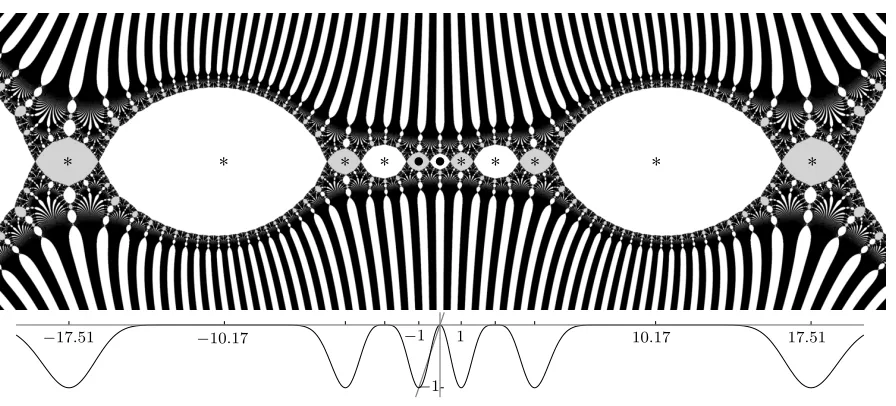
−17.51 −10.17 −1 1 10.17 17.51
[image:23.612.86.534.74.277.2]−1
Figure 5. Illustration of the construction of Example 1.7. Shown are the Julia set and the graph of the function g2 that would arise from the choice of
N1 = 5 and N2 = 25. Note the large size of the Fatou components containing
high-degree critical points. For the actual construction of Example 1.7 the sequence (Nk) has to grow much more rapidly than indicated by the above
values ofN1 and N2.
We begin by outlining the construction, which is based on the idea that a critical point of sufficiently high degree can be used to approximate the behaviour of an asymptotic tract. Indeed, suppose that we start with the Laguerre-P´olya function g0 from the
introduction to this section (wherec±1 =−1 andcn = 0 if|n| 6= 1). The super-attracting
point 0 is an asymptotic value forg0, and sinceJ(g0) intersects the unit disc, there is an
unbounded Fatou component ofg0 that intersects the unit circle Γ1 :={z:|z|= 1}. Let
us modify the sequence c by introducing the additional non-zero points c±N = −1, for
some large integerN. By continuity of the Maclane-Vinberg method, the corresponding functiong1 is close tog0, but has an additional pair of critical points of degreeN−1. It
follows (see below for details) thatg1 can be chosen to have abounded Fatou component
that intersects both Γ1 and Γ2 :={z: |z|= 2}. Asg1 still has an asymptotic value over
0, we can repeat the procedure and create a function g2 that has two Fatou components
both intersecting Γ1 and Γ2. Continuing inductively, in the limit we obtain a functiong
that has no asymptotic values by Lemma 5.1, but has infinitely many Fatou components that intersect both Γ1 and Γ2. ThenJ(g) is not locally connected by Lemma 2.3.
To provide the necessary details, let N = (Nk)k≥0 be a (rapidly) increasing sequence
of odd positive integers with N0 = 1. We define sequences cK (depending on N) by
cKn := (
−1 if |n|=Nk for some 0≤k ≤K
0 otherwise,
and their limit c=c(N),
cn:=
(
−1 if |n|=Nk for some k ≥0
Let gK := gc
K
and g = gN := gc be the corresponding Laguerre-P´olya functions. (See
Figure 5.)
The superattracting fixed points 0 and−1 are the only critical values of gK and of g.
As in the construction of Example 1.6, we find that their immediate attracting basins are bounded by Jordan curves. By Lemma 5.1, g has no asymptotic values, and hence every Fatou component of g is a bounded Jordan domain (Theorem 1.4).
If (ξn)n∈Zis again the sequence of critical points ofg, theng(ξ±Nk) = −1 andg(ξn) = 0 when n 6= |Nk| for all k. In particular, ξNk+1 = · · · = ξNk+1−1 for all k. Let 0 = η0 < η1 < η2 < . . . be the sequence of non-negative preimages of 0; that is ηk =ξNk−1. Also letU(ηk) be the Fatou component of g containingηk. Then g(U(ηk)) =U(0) for k >0.
Our goal is to show that we can choose the sequence N (inductively) so that there is a sequence (αk) of Jordan arcs connecting Γ1 and Γ2 and a sequence (mk) of positive
integers such that gmk(α
k)⊂U(ηk) and hencegmk+1(αk)⊂U(0) for allk. As allαk are
in different Fatou components, this will complete the proof.
In order to define the above sequences, letηK,k, for 0≤k ≤K, denote the critical point
ofgK that corresponds toηk, and letUK(ηK,k) be the component ofF(gK) that contains
ηK,k. We shall construct N, (αk) and (mk) inductively such that gKmk(αk)⊂U(ηK,k) for
K ≥k. The construction will be such that we also have gmk(α
k)⊂U(ηk) for all k.
Suppose that N0, . . . , NK, α1, . . . , αK and m1, . . . , mK have already been chosen, for
some K ≥ 0. As we let NK+1 → ∞, the continuity of the Maclane-Vinberg method
yields that gL → gK for L ≥ K + 1 and g → gK, regardless of the choices of Nl for
l > K+ 1. (Here the convergencegL→gK asNK+1 → ∞is uniformly inL.) Hence, by
choosing NK+1 large, we can achieve that gLmk(αk) ⊂U(ηL,k) for L ≥K + 1, as well as
gmk(α
k)⊂U(ηk), for k = 1, . . . , K. Recall thatgK(x)→0 as x→ ∞, so there isX >0
such that [X,∞) is contained in the basin of attraction of 0 (for gK). Since 0 and −1
are superattracting fixed points of gK, the Julia set J(gK) intersects the unit disc D.
It follows that there is mK+1 >0 and a connected component of g
−mK+1
K [X,∞)
that connects a point in D to ∞. Let αK+1 be a piece of this curve that connects Γ1 to Γ2.
Since gL →gK as NK+1 → ∞, we have ηL,K+1 → ∞ asNK+1 → ∞, uniformly in L,
as well as ηK+1 → ∞. Hence, if NK+1 is chosen sufficiently large, then g
mK+1
L (αK+1)⊂ U(ηL,K+1) and gmK+1(αK+1) ⊂ U(ηK+1). This completes the inductive construction of
Example 1.7.
In both Example 1.6 and Example 1.7, we constructed a function having two super-attracting cycles, at 0 and at −1. Recall that, in both cases, local connectivity of the Julia set failed due to the preimage components of the immediate basin of 0. The role of the fixed point at −1, and its preimages, was to separate 0 from all its preimages, and hence ensure that the immediate basins of attraction are bounded.
We remark that it is possible to modify the constructions to create a map having only a single superattracting fixed point. This is achieved by normalizing our mapsg so that
References
[Ahl78] Lars V. Ahlfors,Complex analysis, third ed., McGraw-Hill Book Co., New York, 1978, An introduction to the theory of analytic functions of one complex variable, International Series in Pure and Applied Mathematics.
[AO93] Jan M. Aarts and Lex G. Oversteegen,The geometry of Julia sets, Trans. Amer. Math. Soc. 338(1993), no. 2, 897–918.
[Bak70] I. Noel Baker,Limit functions and sets of non-normality in iteration theory, Ann. Acad. Sci. Fenn. Ser. A I Math.467(1970), 11.
[BD99] I. Noel Baker and Patricia Dom´ınguez,Boundaries of unbounded Fatou components of entire functions, Ann. Acad. Sci. Fenn. Math.24(1999), no. 2, 437–464.
[BD00a] , Some connectedness properties of Julia sets, Complex Variables Theory Appl. 41 (2000), no. 4, 371–389.
[BD00b] Ranjit Bhattacharjee and Robert L. Devaney,Tying hairs for structurally stable exponentials, Ergodic Theory Dynam. Systems20(2000), no. 6, 1603–1617.
[Ber93] Walter Bergweiler, Iteration of meromorphic functions, Bull. Amer. Math. Soc. (N.S.) 29 (1993), no. 2, 151–188.
[Bis15] Christopher J. Bishop,Constructing entire functions by quasiconformal folding, Acta Math. 215(2015), no. 1, 1–60.
[BM02] Walter Bergweiler and Shunsuke Morosawa, Semihyperbolic entire functions, Nonlinearity 15(2002), no. 5, 1673–1684.
[BM07] Alan F. Beardon and David Minda, The hyperbolic metric and geometric function theory, Quasiconformal mappings and their applications, Narosa, New Delhi, 2007, pp. 9–56. [BR84] I. Noel Baker and Philip J. Rippon,Iteration of exponential functions, Ann. Acad. Sci. Fenn.
Ser. A I Math.9(1984), 49–77.
[BW91] I. Noel Baker and Jonathan M. Weinreich,Boundaries which arise in the dynamics of entire functions, Rev. Roumaine Math. Pures Appl.36(1991), no. 7-8, 413–420, Analyse complexe (Bucharest, 1989).
[CP03] Joan J. Carmona and Christian Pommerenke, Decomposition of continua and prime ends, Comput. Methods Funct. Theory 3(2003), no. 1-2, 253–272.
[Den13] Asli Deniz,Entire trancendental maps with two singular values, Ph.D. thesis, Roskilde Uni-versity and Universitat de Barcelona, 2013.
[Dev84] Robert L. Devaney, Julia sets and bifurcation diagrams for exponential maps, Bull. Amer. Math. Soc. (N.S.)11(1984), no. 1, 167–171.
[DF08] Patricia Dom´ınguez and N´uria Fagella, Residual Julia sets of rational and transcendental functions, Transcendental dynamics and complex analysis, London Math. Soc. Lecture Note Ser., vol. 348, Cambridge Univ. Press, Cambridge, 2008, pp. 138–164.
[DH85] Adrien Douady and John Hamal Hubbard, On the dynamics of polynomial-like mappings, Ann. Sci. ´Ecole Norm. Sup. (4) 18(1985), no. 2, 287–343.
[Dou93] Adrien Douady,Descriptions of compact sets inC, Topological methods in modern mathe-matics (Stony Brook, NY, 1991), Publish or Perish, Houston, TX, 1993, pp. 429–465. [Dra07] David Drasin,Regularity of growth and the classS, Conform. Geom. Dyn.11(2007), 90–100. [DS02] Patricia Dom´ınguez and Guillermo Sienra, A study of the dynamics of λsinz, Internat. J.
Bifur. Chaos Appl. Sci. Engrg.12 (2002), no. 12, 2869–2883.
[EL87] Alexandre E. Eremenko and Mikhail Yu. Lyubich, Examples of entire functions with patho-logical dynamics, J. London Math. Soc. (2)36(1987), no. 3, 458–468.
[EL92] ,Dynamical properties of some classes of entire functions, Ann. Inst. Fourier Grenoble 42(1992), no. 4, 989–1020.
[EY12] Alexandre Eremenko and Peter Yuditskii, Comb functions, Recent advances in orthogonal polynomials, special functions, and their applications, Contemp. Math., vol. 578, Amer. Math. Soc., Providence, RI, 2012, pp. 99–118.
[Fag95] N´uria Fagella, Limiting dynamics for the complex standard family, Internat. J. Bifur. Chaos Appl. Sci. Engrg.5(1995), no. 3, 673–699.
[Fat20] Pierre Fatou, Sur les ´equations fonctionnelles, II., Bull. Soc. Math. Fr. 48 (1920), 33–94 (French).
[GO08] Anatoly A. Goldberg and Iossif V. Ostrovskii,Value distribution of meromorphic functions, Translations of Mathematical Monographs, vol. 236, American Mathematical Society, Prov-idence, RI, 2008, Translated from the 1970 Russian original by Mikhail Ostrovskii, With an appendix by Alexandre Eremenko and James K. Langley.
[G´S97] Jacek Graczyk and Grzegorz ´Swiatek, Generic hyperbolicity in the logistic family, Ann. of Math. (2)146(1997), no. 1, 1–52.
[Hei57] Maurice Heins, Asymptotic spots of entire and meromorphic functions., Ann. of Math. (2) 66(1957), 430–439 (English).
[KSvS07] Oleg Kozlovski, Weixiao Shen, and Sebastian van Strien,Density of hyperbolicity in dimen-sion one, Ann. of Math. (2)166(2007), no. 1, 145–182.
[Lyu97] Mikhail Lyubich, Dynamics of quadratic polynomials. I, II, Acta Math. 178(1997), no. 2, 185–247, 247–297.
[Mac47] Gerald R. MacLane, Concerning the uniformization of certain Riemann surfaces allied to the inverse-cosine and inverse-gamma surfaces, Trans. Amer. Math. Soc.62(1947), 99–113. [MB10] Helena Mihaljevi´c-Brandt,A landing theorem for dynamic rays of geometrically finite entire
functions, J. Lond. Math. Soc. (2)81(2010), no. 3, 696–714.
[MB12] , Semiconjugacies, pinched Cantor bouquets and hyperbolic orbifolds, Trans. Amer. Math. Soc. 364(2012), no. 8, 4053–4083.
[Mer08] Sergei Merenkov,Rapidly growing entire functions with three singular values, Illinois J. Math. 52(2008), no. 2, 473–491.
[Mor99] Shunsuke Morosawa, Local connectedness of Julia sets for transcendental entire functions, Nonlinear analysis and convex analysis (Niigata, 1998), World Sci. Publ., River Edge, NJ, 1999, pp. 266–273.
[MU08] Volker Mayer and Mariusz Urba´nski,Geometric thermodynamic formalism and real analyt-icity for meromorphic functions of finite order, Ergodic Theory Dynam. Systems28(2008), no. 3, 915–946.
[Nad92] Sam B. Nadler, Jr., Continuum theory, Monographs and Textbooks in Pure and Applied Mathematics, vol. 158, Marcel Dekker Inc., New York, 1992, An introduction.
[Obr63] Nikola Obreschkoff, Verteilung und Berechnung der Nullstellen reeller Polynome, VEB Deutscher Verlag der Wissenschaften, Berlin, 1963.
[Osb13] John W. Osborne, Spiders’ webs and locally connected Julia sets of transcendental entire functions, Ergodic Theory Dynam. Systems33(2013), no. 4, 1146–1161.
[Pom92] Christian Pommerenke, Boundary behaviour of conformal maps, Grundlehren der Math-ematischen Wissenschaften [Fundamental Principles of Mathematical Sciences], vol. 299, Springer-Verlag, Berlin, 1992.
[Rem06] Lasse Rempe, Topological dynamics of exponential maps on their escaping sets, Ergodic Theory Dynam. Systems 26(2006), no. 6, 1939–1975.
[Rem08] , On prime ends and local connectivity, Bull. Lond. Math. Soc. 40 (2008), no. 5, 817–826, Updated version available at http://arxiv.org/abs/math/0309022.
[Rem09] ,Rigidity of escaping dynamics for transcendental entire functions, Acta Math.203 (2009), no. 2, 235–267.
[Rem13] Lasse Rempe-Gillen,Hyperbolic entire functions with full hyperbolic dimension and approx-imation by Eremenko–Lyubich functions, Proc. London Math. Soc. (2013).


![1 [(Bromomethyl)(phenyl)methylene] 2 (2,4 dinitrophenyl)hydrazine](data:image/gif;base64,R0lGODlhAQABAIAAAP///wAAACH5BAEAAAAALAAAAAABAAEAAAICRAEAOw==)