A comparative study of analysis methods in quantitative label free proteomics

A Comparative Study of Analysis

Methods in Quantitative Label-free

Proteomics

Thesis submitted in accordance with the requirements of the

University of Liverpool

for the degree of Doctor in Philosophy

by

Katherine Isabella Mackay

Thesis Abstract – A Comparative Study of Analysis Methods

in Quantitative Label-free Proteomics

Katherine Isabella Mackay

The large amounts of data generated by modern proteomics experiments necessitates the use of software pipelines to conduct the bulk of the post-processing. While many software packages (both commercial and open-source) are available to perform some or all of the necessary post-processing steps, it is usual for each research group to use only the instrumentation and software packages with which they are most familiar and/or which are available to analyse their unknown data.

The intention of the studies presented within this thesis was to assess the correlation between the experimental results obtained when;

- a single result dataset is obtained and post-processed in parallel using four separate software pipelines

- a single sample is analysed on two different mass spectrometers and post-processed in parallel

and;

- when different identification thresholds are applied to a dataset prior to parallel quantitation of the resultant data sets

Correlation between different mass spectrometry instruments was assessed and found to yield high r values, especially at the protein level, and was also found to improve following the application of abundance thresholds, however the result of applying score thresholds was unpredictable.

Table of Contents

1 – Introduction

1-35

1.1 Aims and Objectives 1

1.2 Proteomics 1-2

1.3 Proteins 3-5

1.4 Mass Spectrometry 6-17

1.4.1 Ionisation source 7-9

1.4.2 MS analysis (1st _{mass analyser) 9-10}

1.4.3 Fragmentation stage 10-11

1.4.4 MS-MS analysis (2nd _{mass analyser) 11}

1.4.5 Mass analyser types 12-15

1.4.5.1 Time-of-flight (TOF) mass analyser 12-13

1.4.5.2 Iontrap mass analyser 14-15

1.4.5.3 Orbitrap mass analyser 15

1.4.6 LC-MS Output Data 16-17

1.5 Protein Mass Spectrometry 17-22

1.5.1 Analysis of Whole Proteins 18-19

1.5.2 Analysis of Peptides as a Method to Identify Unknown Proteins 20-22 1.6 Identification of Proteins from Peptide MS-MS Data 22-24 1.7 Concatenated target-decoy Database Searching 25-26

1.8 Labelling Techniques in Proteomics 27-30

1.8.1 Stable Isotope Labelling with Amino Acids in Cell Culture (SILAC) 28-29 1.8.2 Isobaric Tags for Relative and Absolute Quantification (iTRAQ) 29

1.8.3 Isotope-coded Affinity Tags (ICATs) 30

1.9 Label-free Proteomics 30-35

1.9.1 Quantitation Methods 31-35

1.9.1.1 Spectral Counting Methods 31-32

1.9.1.2 Intensity Based Methods 32-34

2

– Quantitative Proteomics Software used in

Combination to Reduce False Discovery Rate

36-69

2.1 Aims 36

2.2 Introduction 36-37

2.2.1 Datasets studied 38-39

2.2.1.1 ABRF iPRG2009 38-39

2.2.1.2 CPTAC Study 6 38-39

2.3 Methods 40-49

2.3.1 FASTA files used 41

2.3.1.1 ABRF iPRG2009 data 41

2.3.1.2 CPTAC Study 6 data 41

2.3.2 Software packages used 42-44

2.3.2.1 emPAI calculation 42

2.3.2.2 APEX Quantitative Proteomics Tool 42-43

2.3.2.3 Progenesis LC-MS (Nonlinear Dynamics Ltd) 43-44

2.3.2.4 MaxQuant 44

2.3.3 Median Absolute Deviation Normalisation

(intensity based methods) 44-45

2.3.4 Total Count Normalisation (spectral counting based methods) 45 2.3.5 Thresholds for inclusion of data for analysis 45

2.3.5.1 Heatmap data thresholds 45-46

2.3.5.2 Thresholds for inclusion in pseudo-ROC plots 46

2.3.6 Tests for differential expression 47

2.3.7 Calculating FDR and sensitivity for pseudo-ROC plot generation 47

2.3.8 Consensus across different packages 48-

2.3.8.1 Heatmap generation 48

2.3.8.2 QPROT Z-statistic 49

2.4 Results 49-66

2.4.1 ABRF data 50-52

2.4.2 CPTAC ratio calculation 52-55

2.4.3 Consensus across different tools 56-66

2.4.3.1 Measurement of differential expression by Student’s t-test 56

2.4.3.3 Heatmaps 60-61

2.4.3.4 QPROT post-processing 62-66

2.5 Discussion and Conclusions 67-69

3

– Pairwise comparisons of the results obtained

when using different mass spectrometry platforms

for label-free data

70-97

3.1 Inroduction 70-72

3.2 Methods 71-76

3.3 Results 77-94

3.3.1 Common and unique proteins 77-78

3.3.2 Pearson correlation 79-81

3.3.2.1 Feature data correlation at different thresholds 79-81 3.3.2.2 Protein data correlation at different thresholds 82-86

3.3.3 Coefficient of Variance 87-

3.3.3.1 Feature data 87-90

3.3.3.2 Protein data 90-94

3.4 Discussion and Conclusions 95-97

4

– The effect of the identification thresholds used

on the results obtained from label-free data

98-

4.1 Introduction 98

4.2 Methods 98-99

4.3 Results 100-

4.3.1 Manual peptide FDR thresholds applied to data

searched using Mascot 100-103

4.3.2 Peptide FDR thresholds applied within Scaffold using

Mascot, OMSSA and X!Tandem search results 103-106

5

– Discussion

108-110

5.1 Project overview 108

5.1.1 Achievements 108

5.1.2 Key points highlighted by this project 108-109

5.1.3 Limitations 109-110

5.1.4 Suggestions for future work 110

5.2 Relevance to the field 110

6 – Acknowledgements

111

1

– Introduction

1.1

– Aims and Objectives

The studies described in this thesis aim to explore the assumptions of reliability and comparability applied to label-free proteomics data, and to suggest possible strategies of evaluating and improving on the accuracy of these assumptions. While there is much innovation in the development of new experimental and post processing techniques, there are few published studies investigating these validation questions. Investigations of this nature are however highly relevant to the field of proteomics and the wider field of molecular biology, especially as both the popularity of label-free proteomic methods and the complexity of those biological systems they are applied to increases.

In the process of the studies presented here, as well as investigating the correlation of results obtained using different post-processing methods on the same data (Chapter Two, page 36), and using different instrument platforms with analogous post processing (Chapter Three, page 70), it was also intended to identify and implement relatively simple and practical strategies that increase the confidence of protein identifications, and hence quantitative values, through the use of multiple post processing pipelines (Chapter Two, page 36) in a manner analogous to the improvement observed when using multiple search engines to add confidence to protein identifications by reducing the false discovery rate (FDR)[3].

Throughout the remainder of this introduction I will present the experimental basis of proteomics and MS, the computation techniques available for the identification and quantification of proteins, and the software and instrumentation available.

1.2

– Proteomics

now asked by proteomics are much more complex than simple identification (such as asking which proteins are differentially expressed between healthy and diseased cells, or which proteins are modified in given cellular conditions – e.g. following infection of cells with a parasite). Also, it is now often desired to obtain quantitative information from most proteomic experiments. The increased availability of complex instrumentation for use in proteomics workflows for additional information on the instrumentation available) has led to more research groups using proteomics techniques in their studies, and therefore an increased demand for bioinformatics software to process the resultant data[15].

One of the important issues encountered when asking these more complex biological questions is that the abundance of any given protein within the cell is constantly changing and thus any single experiment will provide only a ‘snapshot’ of the proteins present within that cell at the time of sample collection. While this information is eminently useful for the identification of those proteins present in a given condition, it is necessary to study how protein expression is changing over time in order to obtain a full understanding of the function of proteins within cells and tissues. While time course experiments have been conducted to assess the turnover of proteins within cells[16], this type of study remains expensive and challenging and therefore has not become routine.

1.3 – Proteins

Proteins are biological macromolecules possessed of a multidimensional structure as a function of the chemical composition of their constituent polypeptide regions. Each of these polypeptide regions comprises a polymeric chain of amino acids joined by amide bonds, with terminal carboxylic acid and amine moieties, which are joined via amide bonds to form the peptide backbone. A generalised summary of peptide properties and moieties is shown in Figure 1.

amide bond

carboxylic acid moiety

amine moiety

amide bond

carboxylic acid moiety

amine moiety

Figure 1: Summary of generic peptide properties.

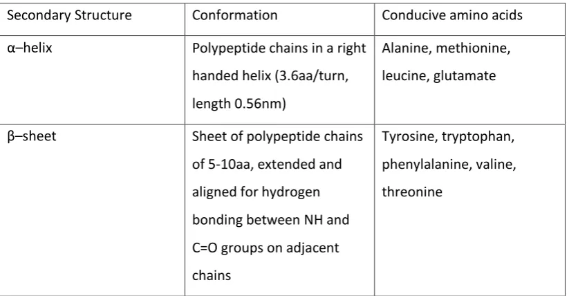
There are 20 main amino acids that combine in various combinations to create proteins, as shown in Table 1. The order of amino acids in the polypeptide chains, and hence in the final protein chain, is denoted as the primary structure of the protein. The functionality (i.e. the side chains present on the peptide backbone) of each amino acid in the chain contributes to the conformation of the protein chain in space via multiple interactions such as Vann der Waals forces and hydrogen bonding. Hydrogen bonding in particular can lead to a very ordered sub-structure in suitable polypeptide regions of the protein chain, with this structure most commonly taking the form of an α–helix or β–sheet (the properties of each of these types of structure are shown in Table 2). This level of order is denoted as the secondary structure of the protein. Both the α–helix and the β–sheet maximise the pairing of available lone pairs of electrons within hydrogen bonds while minimising steric hindrance between the polypeptide chains. A further layer of organisation, denoted the tertiary structure, refers to the way in which the different polypeptide regions are folded in space. This folding is caused mainly by hydrogen bonding, disulphide bonding or hydrophobic interactions, and is solvent and temperature dependent i.e. the structure may breakdown (or denature) when the protein is heated or dissolved in a new solvent for example. The specific folding of the polypeptide chain allows the protein to become biologically active in specific conditions e.g.

Name

Full 1-letter code

Chemical Formula

(Neutral Molecule) Monoisotopic Mass

Alanine A C3H7NO2 71.0372

Arginine R C6H14N4O2 156.1011

Asparagine N C4H8N2O3 114.0429

Aspartic Acid D C4H8NO4 115.0269

Cysteine C C3H7NO2S 103.0092

Glutamic Acid E C5H9NO4 129.0426

Glutamine Q C5H10N2O3 128.0586

Glycine G C2H5NO2 57.0215

Histidine H C6H9N3O2 137.0589

Isoleucine I C6H13NO2 113.0841

Leucine L C6H13NO2 113.0841

Lysine K C6H14N2O2 128.0949

Methionine M C5H11NO2S 131.0405

Phenylalanine F C9H11NO2 147.0684

Proline P C5H9NO2 97.0528

Serine S C3H7NO3 87.0320

Threonine T C4H9NO3 101.0477

Tryptophan W C11H12N2O2 186.0793

Tyrosine Y C9H11NO3 163.0633

Valine V C5H11NO2 99.0684

Secondary Structure Conformation Conducive amino acids α–helix Polypeptide chains in a right

handed helix (3.6aa/turn, length 0.56nm)

Alanine, methionine, leucine, glutamate

β–sheet Sheet of polypeptide chains

of 5-10aa, extended and aligned for hydrogen bonding between NH and C=O groups on adjacent chains

[image:12.595.114.526.70.284.2]

Tyrosine, tryptophan, phenylalanine, valine, threonine

1.4 - Mass Spectrometry

Mass spectrometry essentially involves the measurement of the mass to charge (m/z) ratio of ions within a vacuum. With the exception of time-of-flight instruments and magnetic sector instruments (which are now rarely used), this is achieved via the application of RF and dc voltages to create an electric field in which there is a stable path for only those ions of a specific mass and charge. The mass spectrometry instrument scans sequentially through each mass in a user specified mass range (e.g. 300-3000amu) to identify those analyte ions which are present in the sample.

The original mass spectrometry instruments merely ionised the sample and ‘weighed’ the ions produced, however it is now more usual to see ‘hybrid instruments’ which involve a fragmentation stage and thus provide more information about the sub-structure of the ions of interest through the study of (fragment) daughter ions. Though there are several methods of ionisation and mass analysis, the general schematic of the hybrid mass spectrometer remains the same, and is shown Figure 2.

ionisation source

atmospheric

pressure Vacuum Stages

Fragmentation

stage 2nd mass analyser

1st mass analyser Dectector

ionisation source

atmospheric

pressure Vacuum Stages

Fragmentation

stage 2nd mass analyser

1st mass analyser Dectector

1.4.1 - Ionisation source:-

The ionisation source of choice for the quantitative study of proteins is the nano-electrospray source[25], based upon the standard electrospray source but able to deal with the smaller sample volumes available. Electrospray (ESI) is referred to as a ‘soft’ ionisation method, with ionisation occurring directly from the sample solution at atmospheric pressure. The ions are then passed through a transition section de-pressurised by a roughing pump and from there into the high vacuum stages which contain the mass analyser and detector. ‘Soft ionisation’ refers to any ionisation method which produces primarily [M+H]+ _{ions with minimal fragmentation; this is especially useful when studying}

unknown analytes as it prevents confusion between parent and daughter ions at the full scan stage (“full scan” refers to a scan which records all ions present with a m/z ratio within the user specified scan range). Manufacturers provide many subtle variations on the basic electrospray ionisation source, however the general principles of operation remain the same. Within the ionisation source the sample solution (a polar solvent in which the sample is soluble) is nebulised from a capillary tube into the source housing via a needle which is held at high potential. The potential difference between the needle and a counter electrode causes charge separation within the liquid and subsequent deformation of the meniscus at the needle end to form a cone (the ‘Taylor cone’)[26, 27] as shown in Figure 3. At the apex of this cone the charge density is very high and a fine jet of charged liquid is ejected towards the counter electrode. This jet cannot remain stable and breaks up further into charged droplets, which are driven apart by Coulombic repulsion to produce a mist of smaller charged droplets containing the ions which were pre-formed in the polar sample solution.

Excess charge density moves to the surface of these droplets as a conducting medium, with the surface charge density increasing as solvent ions are evaporated to give progressively smaller droplets[28]. At some point the surface charge density has increased such that the repulsive Coulombic forces between analyte ions become stronger than the force of the surface tension which binds the droplet together (this point is known as the Rayleigh stability limit). When this point is reached it causes the droplet to ‘explode’ in a process called Coulombic Fission, which occurs multiple times to produce steadily smaller droplets. Some theories suggested that this Coulombic Fission simply continues until repulsive forces cause the droplet to break up, giving both free and cluster (adduct) ions in the form of charged ‘droplets’ which inherit the charge of the parent droplet (the Charged-Residue model). More recent studies have suggested that the droplets do not in fact ‘explode’, but instead eject smaller droplets in a process known as ‘droplet jet fission’[29]. This occurs from the elongated end of the microdroplets that are deformed by their flight under the influence of the electric field. The charge density is significantly increased in this area of elongation and a jet of smaller daughter droplets is produced in a process analogous to the formation of the original jet emitted from the Taylor cone at the mouth of the capillary. The daughter droplets formed account for approximately 1-2% of the mass, but 10-18% of the charge of the parent droplet, and are therefore subject to an increased surface charge density[26].

It has also been suggested, by J. Iribarne et al, that when a certain radius is reached, ion evaporation becomes favourable over Coulombic Fission and free analyte ions are evaporated from the surface of the droplets – their study calculated this point to equate to a surface charge density of approximately 108_Vcm-3 _{(this is termed the Ion Evaporation}

model)[30]. Though there is a continuing debate on the exact method of formation of ions in ESI, it is generally assumed that the CRM is more appropriate for large molecules and the IEM for small molecules, though in actuality the method of formation is likely to be a hybrid of these two models.

the mass spectrometer to liquid chromatography (LC), with the added advantage of increased sample separation and purification of the individual components of the sample into separate chromatographic peaks. Thus in addition to ionization mode, the choice of solvent used in the LC stage should also be carefully considered in terms of ionisation suitability, as well as chromatographic efficiency, as the more ‘hydrophobic’ an analyte is in a given solvent, the easier it will be to overcome the solvation energy and the ions will be more easily desorbed into the gas phase[28, 31, 32]. However this must be traded with the ability of analyte molecules to form ions or at least strong dipoles in the solvent solution, which enhances ion abundance[29]. Taking both considerations into account, it can be seen that choosing the correct solvent can therefore have a significant effect on the efficiency of ionisation, and the ideal parameters will vary greatly for different analytes. Therefore all solvent characteristics should be optimised for specific analytes – including the pH of the chromatographic mobile phases (as positive ions are most readily formed in acidic solutions and vice versa).

Once desorbed within the electrospray source, the free analyte ions (and any analyte adduct ions) are drawn into the mass spectrometer via the ion sweep cone and passed into the 1st

mass analyser.

1.4.2 - MS analysis (1st mass analyser):- The 1st _{mass analyser conducts full scan MS analysis,}

recording the analyte ions according to their m/z ratio. In almost all hybrid instruments this first stage will involve a quadrupole mass analyser.

The four rods in the quadrupole are divided electrically into two pairs, with the voltages applied to each rod pair being equal in amplitude but opposite in sign. The quadrupoles repeatedly ‘scan’ through the specified mass spectrum (e.g. 300-3000 atomic mass units) by altering the RF and dc voltages applied to each of the quadrupole rod pairs. Each RF/dc voltage combination will create a stable path through the quadrupole for ions of a certain m/z only (such a stable path is shown in Figure 4), with ions of all other m/z values following a collisionary path and being neutralised (by collision with the rods) or ejected from the cell (by passing out between the rods).

In hybrid instruments with multiple mass analyser stages, the first stage of mass analysis within the quadrupole mass analyser can be used for mass scanning where parent masses are measured without collecting fragmentation data; however in the time-of-flight or orbitrap instruments often used for proteomics it is generally desired to exploit the higher mass resolution of these mass analysers to gain accurate mass data for the parent ions (and hence greater confidence in their identification). In this situation the quadrupole functions as an ion transfer device in the first stage of mass analysis, creating a stable path for all ions within the specified mass range and thus passing them forward to the TOF or orbitrap mass analyser for full scan mass analysis of the parent ions.

increases the translational kinetic energy of the ions as they enter the collision cell. As the translational kinetic energy of the ions increases, so does the amount of energy transferred in any given collision and consequently the degree of fragmentation will increase with increased collision energy. Optimisation of the collision energy aims to maximise the production of diagnostic fragments – it becomes difficult to resolve the structure of large fragments as the possible ion combinations to produce a given m/z ratio increases, and small fragments eventually become too common to use in structure elucidation. To ensure there is no crossover of fragments between parent ion masses it is usual for the collision cell to be purged of ions between scans by applying a large voltage of the opposite polarity to the rod pairs.

1.4.5 - Mass Analyser Types

1.4.5.1 - Time-of-flight (TOF) mass analyser:- The TOF mass analyser measures m/z as a function of the ‘drift time’ of a given ion within a flight tube of specific length, when accelerated towards a detector under vacuum conditions.

Before entering the flight tube, ions are accumulated in the collision cell via the application of a voltage of the same polarity as the analyte ions to the end gate of the collision cell, which repells the ions from the gate. These accumulated fragment ions are then allowed into the flight tube to coincide with the next TOF-pulse, by swapping the polarity on the end gate to allow the ions to move out of the collision cell.

The TOF-pulse itself is created by the application of a strong voltage of the same polarity as the analyte ions to orthogonal accelerator (pulsar) plates - this propels the ions out of the end gate towards the detector. In modern instruments the ions often reach the detector not by a linear flight path but via a reflector, or in some cases several reflectors, which serve to normalise the energy difference between ions of identical mass but differing kinetic energy, and also allows the flight tube section of the instrument to remain physically the same size despite increasing the length of the flight path for ions[37]. The reflector itself is a set of plates charged with the same polarity as the analyte ions, which ‘reflects’ the ions towards the detector by electrical repulsion. Normalisation is achieved as those ions with higher kinetic energy will penetrate further towards the plates and lose their ‘excess’ energy through repulsion. Thus all ions of the same m/z ratio are caused to reach the detector after the same drift time within the flight tube. A schematic of a TOF-analyser containing a single reflector is shown in Figure 5.

[image:20.595.124.362.76.423.2]

[image:21.595.117.524.156.506.2]

1.4.5.2 - Iontrap mass analyser:- The term ‘ion-trap’ describes a group of mass analysers including linear and three-dimensional ion-traps. A general schematic for each of these is shown in Figure 6.

Figure 6: Geometry of the three-dimensional and linear ion-trap mass analyser[39].

The general principle of both iontrap analyser types remains the same, in that ions are trapped within the electrodes as a function of their mass and charge. By altering the applied RF and dc voltages to create potential wells of stability for ions with a selected m/z ratio only, the full mass spectrum may be scanned by sequentially ejecting ions of particular m/z ratios to the detector. Alternatively, as a collision gas is present, ions of a particular m/z ratio may be trapped, accumulated (with the ejection of all other ions), and fragmented with the resultant fragment ions then being scanned out to the detector. The fact that fragmentation and scanning can occur in the same mass analyser allows for multiple levels of analysis, i.e. it is possible to excite and fragment the first, second, etc level fragment ions (this capability is described as MSn_{) as well as the original parent ions. This may be done by selecting the}

allowing the instrument to select for fragmentation those ions that are observed at the highest ion intensity.

1.4.5.3 - Orbitrap mass analyser:- The orbitrap mass analyser was introduced by Makarov[40] and is a modification of the quadrupole iontrap mass analyser. It is often interfaced with a linear iontrap, which performs the fragmentation stage (as fragmentation within the orbitrap is slow) and mass analysis of the fragment ions, with the orbitrap being used due to its ability to provide high mass resolution for the parent ions. The functional principles are similar to those which describe the iontrap mass analyser, however an electrostatic field (applied dc voltage) only is used to create a stable path for the ions of interest, without the use of RF voltages. The analyser is composed of a spindle electrode and a pair of bell shaped outer electrodes, with the pair being separated by a ceramic insulation ring[41]. A schematic showing the spindle and bell electrodes, as well as the trajectory of trapped ions within them, is shown in Figure 7.

Figure 7: Trajectory path of trapped ions within the orbi-trap mass analyser[42].

1.4.6 LC-MS Output Data

As the sample passes first through a chromatography column before reaching the mass spectrometer, there is chromatographic separation of the individual molecules in the sample prior to ionisation. As each peak i.e. peptide (or group of peptides, when several peptides have the same or very similar physico-chemical properties) elutes from the chromatography column it passes into the ion source of the mass spectrometer. Therefore each elution peak from the chromatography system contains a “packet” of molecules, which are ionised and subsequently recorded at the detector as a peak in the ion abundance. This is reflected in the LC-MS data output, which is known as the total ion chromatogram (TIC)[26]. As the mass spectrometer performs scans, it produces one mass spectrum per scan that shows the m/z ratios of the ions observed in that scan. The total ion abundance recorded in each scan is shown in the TIC, as a function of the retention time[26].

From the TIC, it is possible to computationally construct an extracted ion chromatogram (XIC or EIC) that shows the elution profile only for those sample ions with a user selected m/z ratio. The XIC can be useful to identify related sample molecules, for example one that has been deuterated versus one that has not, that have different m/z ratios but the same elution profile. Using this simple derivatisation strategy it is possible to assess the relative amounts of an analyte in different conditions by performing deuterium exchange on only one of the samples. This will give two peaks in the mass spectrum which are separated by a known mass difference (deuterium is the 'heavy' isotope of hydrogen, possessing a neutron in the nucleus in addition to the proton and electron found in hydrogen and therefore having an atomic mass of 2 – this gives rise to a mass shift of 1 mass unit for each deuterium atom present when studying singly charged molecules).

The mass spectra recorded throughout the TIC can be viewed and analysed to determine which ions are present in each scan[26, 43]. However, rather than a single peak for each ion present, the mass spectrum will show an isotope pattern of several peaks. This is due to the presence of less common isotopes present within the molecule at natural ratios, for example C13 _{and to a lesser extent N}15_{. This isotope pattern includes the monoisoptopic peak, which}

corresponds to the presence of the most abundant isotopes (eg C12 _{and N}14_{), and less intense}

[image:24.595.112.454.135.347.2]

abundance of the peaks mirroring the naturally occurring distribution of those isotopes present). An example isotope pattern is shown in Figure 8.

Figure 8: An example isotope pattern, for the given protein (generated using the IPC (Isotope Pattern Calculator) tool[44].

1.5 - Protein Mass Spectrometry

1.5.1 – Analysis of Whole Proteins

The mass spectrometric analysis of whole proteins may be conducted using ESI, however more usually a iso (Matrix-Assisted Laser Desorption Ionisation) ionisation source is used. Laser desorption ionisation (LDI) was first introduced in the late 1960s[26], and was readily applicable to the analysis of organic salts (low-mass) and light absorbing compounds. However there was not utility to apply this method to protein analysis until the late 1980s, as it was non-trivial to obtain useful spectra for biomolecules, especially those with mass exceeding 2000 atomic mass units. Two methods were put forward that allowed analysis of biomolecules via LDI; the mixture of the analyte (in glycerine) with ultrafine cobalt power, and the co-crystalisation of the analyte with an organic matrix (MALDI). This second method gained more use as it gave greater sensitivity and versatility as a technique, though both methods are capable of producing useful spectra for molecules with molecular weight up to 100000 atomic mass units.

attenuation may be optimised for each measurement. A schematic of the MALDI ionisation source is shown in Figure 9.

Figure 9: Schematic of the MALDI ionisation source[26].

1.5.2 – Analysis of Peptides as a Method to Identify Unknown Proteins

Previously unidentified proteins in complex mixtures can be detected and sequenced using a complex strategy, which involves tandem mass spectrometry utilising the MS-MS functionality of hybrid mass spectrometers with a nano-ESI ion source. Prior to analysis the sample protein mixture is digested with a protease enzyme - most usually trypsin, which according to the Kiel rule “cuts” the protein at the C-terminal end of arginine and lysine peptide residues, but not before proline residues[49]. However cleavages before proline have been described experimentally and the suggestion made that excluding the resultant peptides from the pool of theoretical peptides may prevent the identification of peptides which are in fact present in the sample[49]. In addition, variation in the peptides produced following trypsin digestion may be introduced when the protein sample is not completely digested leading to “missed cleavages”, where a potential cleavage site is missed giving one larger peptide where two smaller peptides would be expected. Therefore the algorithms used must be capable of considering the possible variations to “perfect” digestion. However, it has also been observed that there is no significant difference in precision, accuracy, specificity or sensitivity on the inclusion or exclusion of peptides resulting from missed cleavages[50].

Both proteins and peptides are predominantly protonated on the amino groups during ESI/nano-ESI, i.e. at the N-terminus and on arginyl, histidyl and lysyl residues[51]. Most usually singly charged peptides are observed, though 2+ _{and 3}+ _{charge states are also}

common[51], and whole proteins have been shown to gain approximately one charge per kDa mass[51]. As a general rule for ESI, the signal seen by the mass spectrometer is proportional to the concentration of analyte in the sample[26, 51] and this relationship is flow-rate independent. However this relationship may be affected by the ionization efficiency of the individual peptides, which can give a more confused picture of protein abundance as the intensity of signal from individual peptides may differ even when they arise from the same parent protein molecule present at a given true abundance.

During the second stage of analysis within the collision cell the peptides fragment predominantly at the amide bonds, producing smaller amino acid chain daughter fragments. The main ion types which are produced as a result of fragmentation at standard collision energies have been classified as b- and y-ions. The y-ions arise sequentially from the C-terminus of the parent peptide ion, with y1 describing the amino acid lost if the first amide

bond is cleaved and so on. Correspondingly the b-ions arise from the N-terminus of the peptide ion, again with b1 describing the amino acid lost if the first amide bond is cleaved.

The sites of fragmentation at the amide bond that create both b- and y-ions are shown in Figure 10.

Figure 10: Peptide fragmentation at the amide bond to produce b and y ions[52].

study, the terms feature and peptide-level data can be considered synonyms. However, there are packages that can treat features and peptides differently, for example in the case of two different charge states for the same peptide – where these would be treated as two features, but aggregate values used to give a single peptide.

1.6 - Identification of Proteins from Peptide MS-MS data

Though this originally involved de novo sequencing from manual analysis of the data, as is done for the analysis of small molecules[24, 53], it is now more usual to use database searching software for protein inference. This increases the automation of proteomic experiments and greatly decreases the time required for this step, therefore bringing the analysis of hundreds of unknown proteins into the realms of practicability. A summary of the steps involved in this automated process is shown in Figure 11.

[image:31.595.116.459.75.765.2]

1.7 - Concatenated target-decoy Database Searching

While it is possible to assign protein probabilities calculated from the peptide probabilities of the assigned constituent peptides[54], as implemented in the Trans Proteomic Pipeline web based software, it is increasingly common for a concatenated target-decoy database to be used so that it is possible to calculate a false discovery rate (FDR)[55] as a measure of confidence.

The concatenated target-decoy database is created from original .fasta files containing all the proteins predicted from gene models of the organisms being studied (if more than one organism is present, e.g. when studying the infection of human cells with a parasite, the .fasta files for all the species present are concatenated into one larger .fasta file). The decoy section of the concatenated target-decoy database is most usually created by appending either a reverse set of all the proteins in the .fasta file (generated by reversing the peptide sequences of the predicted proteins present in the original .fasta file), or a set of artificial protein accessions that are assigned to random peptide sequences. The decoy sequences are clearly denoted as such in the target-decoy database .fasta file, most usually by including a “Decoy” or “REV” suffix concatenated with the accession number of the real sequence, or for randomised concatenated target-decoy databases a “random” prefix with an arbitrary unique identifier (such as a letter or a number) may be used. This method of including equal numbers of target and decoy protein sequences in a single file means that there is equal competition between the real and the decoy sequences, with no bias towards either group.

1.8 - Labelling Techniques in Proteomics

Though this thesis is concerned with the bioinformatics methods used in the context of label-free proteomics, it is useful to include an explanation of common labelling techniques within this introduction to provide context for the term “label-free”. “Labelling” is the term used to describe the derivatisation of the sample molecules in order to differentiate between samples from different conditions, e.g. before and after drug administration, and may be achieved through in vivo metabolic labelling or in vitro chemical labelling[15]. Each of these has its own advantages and disadvantages; in vivo labelling is more efficient and yet prohibitively expensive for some studies (e.g. when looking at a whole complex organism such as a chicken[56]), while in vitro labelling can theoretically be applied to any sample[15].

[image:35.595.112.370.120.385.2]

1.8.1 - Stable Isotope Labelling with Amino Acids in Cell Culture (SILAC)

Figure 12: Example SILAC work flow.

This type of labelling experiment is particularly useful when studying cells in different conditions, e.g. when looking at the effect of drug treatment or the changes following infection with a parasite, and a summary of an example workflow is shown in Figure 12. The cells in condition one are grown in standard media and those in condition two are grown in labelled media, i.e. media containing the heavy isotopes of one or more element within the media such as deuterium or 18_{O. The samples from each condition are then pooled together}

While the least expensive labelling strategy is to use deuterated amino acids, several other labelling atoms are routinely used with the most common strategies using 13_{C and} 15_N

labelled amino acids which give rise to a larger mass shift. This larger mass shift between paired peaks makes it easier to separate out those paired peaks from a complex mass spectrum. As the labelled and unlabelled amino acids experience the same chromatographic and ionisation conditions these fold change values are highly reliable and it is this accuracy which means that SILAC is one of the most commonly used proteomic techniques.

1.8.2 - Isobaric Tags for Relative and Absolute Quantification (iTRAQ)

1.8.3 - Isotope-coded Affinity Tags (ICATs)

The ICAT[58] method also utilises synthetic molecules to derivatise the proteins in the sample. The ICAT reagents have three specific chemical regions: a reactive section, an isotopically coded linker section, and an affinity tag. Once again the technique is designed to find differential expression between two conditions, but this time both samples are derivatised. The sample from one condition is labelled with the heavy form of the reagent and the sample from the other condition is labelled with the light form of the reagent. In both cases the reagent binds to the side chains of cysteinyl residues in the reduced protein samples. The two samples are then pooled and digested to peptides, and the tagged peptides are then isolated by avidin affinity chromatography. The isolated peptides are then analysed by mass spectrometry, with the identification completed as above from the MS-MS spectra and the differential expression inferred from the intensity ratios between the heavy and light peak pairs in the MS spectra. While effective, this technique by its nature cannot quantify cysteine-free proteins and as the cysteine content of proteins is often low this lowers its utility in practice with real samples.

1.9 - Label-free Proteomics

There are two main limitations to the labelling techniques used in proteomics; the first is the high cost of labelled media and the second is the large amount of time taken to prepare fully labelled biological samples.

Label-free quantitation is achieved via direct comparison of the LC-MS-MS data from several runs, and this means that in order to obtain meaningful results it is necessary that the instruments used are capable of delivering extremely high mass accuracy and reproducible chromatography retention times to allow the separate samples to be accurately compared across runs.

1.9.1 - Quantitation Methods

Quantitation for both labelled and label-free methods is typically carried out either via the analysis of extracted ion chromatograms (XICs) to give intensity values (as peak height or area – these are known as intensity based methods)[59] or by using the number of fragmentation spectra matched to peptides as a proxy for the protein abundance in the sample (these are known as spectral counting methods)[60].

1.9.1.1 – Spectral Counting Methods

efficiencies based on the peptide properties (hydrophobicity etc) and using machine learning techniques, such as in the APEX Quantitative Proteomics Tool[64, 65] (which does both).

1.9.1.2 – Intensity Based Methods

Intensity based quantitation is achieved via calculation of the peak height or area for each peptide taken from the MS spectra for that parent mass once the peptide has been identified from the MS-MS spectra. The intensity recorded for each peptide will be a summation of the intensities for all ions present for that peptide, e.g. 1+ _{and 2}+ _{ions. A ratio is calculated for}

each peptide based on the intensities found in each condition, and protein fold change obtained from combining the peptide ratios for all peptides assigned to that protein[61]. This technique requires accurate parent mass values, in order to minimise the issue of peptides of similar mass and eluting together (either in the same peak or in overlapping peaks) being quantified as one peptide.

Recently, there has been a move towards quantification of label-free data via the alignment of accurate mass and retention time across multiple runs to form an aggregate spectrum[66], and a typical work flow for this alignment process is described below;

1. Signal pre-processing

2. Feature detection and quantitation

Peaks present in the TIC are converted to two-dimensional centroid data, and those groups of centroid “peaks” which resemble an isotope pattern are selected for analysis[67]. Each isotope pattern will be present in a number of consecutive scans, for the duration of the elution profile of the chromatographic peak containing the peptide. Once detected, features are quantified by modelling the peak as a Gaussian distribution and calculating the area under the curve. This is broadly correct, however chromatographic peaks will show some tailing effects and there are some more complex algorithms which model this behaviour in order to achieve greater accuracy.

3. Retention time alignment

This alignment step aims to remove variation introduced by differences in retention time between runs, which could be caused by slight temperature or pressure differences within the LC instrument. The alignment step brings those features with the same m/z ratio to a common retention time. This can be done using either signal or identity based methods[68, 69].

4. Collection of peptides across runs

5. Peptide identification mapping

At this stage the identified features are tied to theoretical peptides generated as constituents of those proteins which may be present in the sample, via the accurate mass values assigned to the features (see pages 21-23).

6. Peptide to protein quantitation inference

For label-free methods protein quantitation is usually inferred from the summation of the intensity values assigned to the constituent peptides of that protein, though a mean value may be used. For SILAC (see pages 26-27 for a detailed discussion of the SILAC method) a median ratio is normally used. When peptides cannot be resolved to a single protein it is usual to assign and quantify a protein group instead, to avoid discarding data.

7. Intensity normalisation

A normalisation step is necessary as the total ion count will vary from run to run, and therefore the signal intensities reported from each run (being a proportion of the total ion count) will also vary. Normalisation steps aim to minimise this variation so that the separate runs are comparable, using either internal standards or statistical methods. One possible statistical method (which is used later in this thesis – see page 36) is median absolute deviation (MAD) normalisation[70]. The intensity normalisation step has the potential to greatly affect the intensity values calculated for peptides, and hence proteins, and therefore optimisation of this step is extremely important. Since the work presented in this thesis was conducted, there have been several studies which have looked at optimising the normalisation step[71-73].

1.9.2 – Available Quantitation Software

who wish to use in house or third party search engines. For those who wish use the same software across multiple instrument platforms it is important that there are software packages which are not instrument or input format specific, and packages such as Progenesis LC-MS are becoming more universal as they work to provide this. One issue arising from the large range of software packages available is the lack of standardised data formats, meaning that not all software packages can be used to analyse data from all platforms and therefore this must be considered when designing an experimental pipeline. However conversion scripts/software is emerging to allow simpler transition between data formats, allowing more freedom for analysts to choose a preferred search engine and processing software with which to analyse their data and making comparison between results from different platforms possible[15] and indeed practicable.

In addition to post-processing software the high complexity of samples where the ground truth is unknown means that benchmarking studies using sufficiently complex and truly representative standard datasets are increasingly important in order to add confidence to the methods used and hence to the biological conclusions made from the experimental results. As the creation of such standard datasets is extremely non-trivial, it will be highly beneficial to the field if these datasets once created are made freely available from online repositories, such as the NCCR Yeast Resource Centre Public Data Repository[4], PRIDE[5], the Global Proteome Machine Database (GMPdb)[6], PeptideAtlas[7], MassIVE (UCSD)[8], or Tranche[9], as the availability of good datasets will allow a greater number of

meaningful benchmarking studies to be conducted by bioinformaticians and

experimentalists who may not have the expertise, time or equipment required to design and prepare the complex standard samples themselves. This ready availability of

proteomics datasets in standard open-source formats is the aim of the ProteomeXchange (PX) consortium[10], which currently includes PRIDE[5], PeptideAtlas[7] and MassIVE (UCSD)[8]. Another consideration of great importance is the need for long term stability of proteome repositories to avoid the loss of datasets, for example many researchers

2 - Quantitative Proteomics Software used in Combination to

Reduce False Discovery Rate

2.1 - Aims

This software comparison study aims to determine how much variability is introduced into final results through the use of different software pipelines to analyse the same data set, in terms of the number of proteins reported as differentially expressed, which proteins are identified/quantified, and the false discovery rate for each pipeline. As well as comparing and contrasting results from individual pipelines, the pipelines used allow comparison of intensity-based label free pipelines versus spectral counting pipelines, and in addition this study examines the potential of creating a consensus method which takes data from all pipelines to produce a more robust result than any single pipeline alone.

2.2 - Introduction

The quantitation methods considered in this study are; emPAI[83] values generated within and reported by Mascot (Matrix Science), spectral count and intensity values reported from Progenesis LCMS (Non-Linear Dynamics), absolute protein expression values from the APEX quantitative proteomics tool[64, 84] (following processing using the Trans-Proteomic Pipeline[85] web interface), and intensity values from MaxQuant[86] (open source). Very little work has been done where this type of comparison has been made between different spectral counting and intensity based software pipelines[87], with discussions of this type largely restricted to the presentation or comparison of novel in-house pipelines with those which are more widely used (both intensity based[88-92] and spectral counting based[93, 94] workflows) rather than an assessment of the software pipelines that are available to the standard user. Despite this, an investigation of the reliability of those software pipelines used for the analysis of proteomic data is an extremely important research question, and increasingly so as these methods become more widely used, and the biological questions asked by these analyses becomes more complex.

2.2.1 - Datasets studied

2.2.1.1 - ABRF iPRG2009

This dataset was created for an iPRG (Proteome Informatics Research Group) study conducted by the ABRF (Association of Biomolecular Resource Facilities) in 2009, the primary goal of which was to “Evaluate protein differentiation tools for MSMS”, with the additional secondary goal to produce a “benchmark reference” of ‘true’ proteins which could then be used as a basis for software development”[95]. Thus the study was not intended to be quantitative, and therefore the dataset was not constructed with complete quantitative analysis in mind. Thirty different labs took part in the 2009 study, and between them they returned 37 submissions of results. Each submission detailed which proteins had been assigned as significantly changed between the two conditions studied, plus a score showing the confidence placed on each reported protein assignment.

remaining 8% made up from proteins which were agreed upon by a minimum of 2 group members and fell within the expected mass range.

2.2.1.2 – CPTAC Study 6

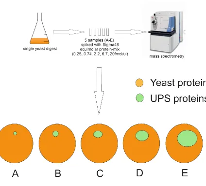
This standard dataset was created for CPTAC (Clinical Proteomic Tumour Analysis Consortium) study 6[96] (published October 2009), which was a benchmarking study seeking to provide a basis which would allow groups to self-assess the performance of their instrumentation and post-processing procedures on a standard dataset where the ground truth is known. The dataset presented consisted of five samples which were the result of splitting a single yeast culture, with the intention to obtain a truly homologous sample as the basis for the prepared standard samples, so that the only difference between the final samples would be the level of spike-in proteins added. Creation of this single culture for use in the study was outsourced by the study group, and was conducted as follows; “S. cerevisiae strain BY4741 (MATa, leu2_0, met15_0, ura3_0, his3_1) was grown in a 10-liter batch of rich (yeast extract peptone dextrose) medium at 30 °C in a fermentor to an A600 of 0.93”[96]. The

sample was then passed back to the study group as a lyophilised yeast lysate, which was reconstituted, reduced and alkylated prior to trypsin digestion. Following digestion the sample (dried digest re-suspended to a concentration corresponding to ~60ng/µl yeast protein before digestion in 0.1% aqueous formic acid) was split into five smaller samples, each of which was spiked with different levels of a standard protein mix (which had also been pre-digested with trypsin). The mix used was the Universal Proteomics Standard 1 (UPS1) standard mix from Sigma-Aldrich[97] (an equimolar protein mix with all proteins present at 5pmols), which was spiked in at a level corresponding to concentrations of 0.25, 0.74, 2.2, 6.7 and 20fmol/µl total protein pre-digestion. This methodology is summarised below in Figure 13.

[image:47.595.124.549.148.532.2]

quantified accurately for the UPS proteins, but that these proteins could not be detected in the A sample (hence only samples B-E are used in this analysis), and that the yeast proteins were not seen to be significantly changing between the 5 samples.

Figure 13: CPTAC samples were created by splitting a single yeast digest into five and spiking each with protein mix (0.25, 0.74,

2.2, 6.7 and 20fmol/ul respectively for samples A-E).

2.3 - Methods

For ease of reference, a workflow diagram has been prepared which summarises the work that has been carried out in the course of this study and this is presented below in Figure 14.

Figure 14: Workflow diagram showing the different stages of analysis for the ABRF and CPTAC data

2.3.1 - FASTA files used

2.3.1.1 – ABRF iPRG2009 data

The official .fasta file distributed via Tranche was used for the analysis of this dataset, with the same .fasta file being input to all software analysis pipelines.

2.3.1.2 - CPTAC Study 6 data

2.3.2 - Software packages used

2.3.2.1 - emPAI calculation

.fasta files were searched using an in-house Mascot server with the following settings: allow 1 missed cleavage, fixed modifications: Carbamidomethyl (C), variable modifications: Oxidation (M)*, Peptide Tolerance: +/-10ppm, MS-MS tol. +/-0.6Da (the fixed and variable modifications are set as a function of the experimental preparation). The emPAI values used were those exported directly from Mascot. The emPAI value is a modification of simple spectral counting, the basic assumption of which is that if a protein is abundantly present all the constituent peptides of that protein will be observed during mass spectrometry. In order to determine the emPAI value, the PAI (protein abundance index) is first calculated by dividing the “observed” value by the “observable” value for each protein in a sample, where the observed value is the number of non-redundant peptides identified (allowing multiple charge states for each peptide) as experimentally associated with that protein and the observable value is the number of peptides per protein predicted from a theoretical digest which are within the defined scan range of the instrument (in the Mascot implementation this range is not simply that set by the user, but is dependent on the highest and lowest m/z values detected experimentally i.e. any theoretical peptides above or below these will not be included in the observable value used in the calculation). The emPAI value is then calculated from the PAI as

𝑒𝑚𝑃𝐴𝐼 = 10𝑜𝑏𝑠𝑒𝑟𝑣𝑎𝑏𝑙𝑒 𝑜𝑏𝑠𝑒𝑟𝑣𝑒𝑑 − 1_.

*The fixed modifications set are a function of the experimental procedure conducted in the sample

preparation, namely reduction and alkylation. The variable modification of oxidation on methionine

is set as this is a common post-translational modification and it is desired to record any proteins

whether they have this modification or not.

2.3.2.2 – APEX Quantitative Proteomics Tool

In the TPP web interface the files were converted to .mzXML and the in-house Mascot server used for the searches (with the same parameters as above). The Mascot result files were then converted to .pepXML files and these were run through the next stage of the TPP, PeptideProphet, with the option selected to run ProteinProphet afterwards (using pI, hydrophobicity and RT information, and including results with pepProphet probability <0.05 and minimum peptide length = 7). The final .protXML files were then analysed using the APEX tool. One .protXML file was selected to be used for training (using the default random forest machine learning algorithm[99], which is considered to be the most appropriate training mechanism for APEX), with reference to the relevant .fasta database file, using the default settings (Consecutive Misses: 0, Use Minimum Peptide Length: 3, Use Minimum Peptide Mass: 250, Use Maximum Peptide Mass 7500, P(i)=1.00, APEX normalisation factor = 0.00) and with all the available peptide properties used to assess the ionisation efficiency of theoretical peptides. This creates an .ARFF file of training data, which is then used with the relevant FASTA file to create an .oi file. This .oi file stores the signal intensity and physico-chemical properties of the peptides found in the training file, and is used as the reference for the analysis of other sample files. The APEX scores are internally calculated using the following formula.

ni = observed spectral counts pi = protein identification probability

Oi = predicted count for one molecule of protein (sum of peptide detection probabilities)

The APEX score, pi, ni and oi are reported in the APEX output .csv file, which can easily be

copied into Excel for post-processing.

2.3.2.3 - Progenesis LC-MS (Nonlinear Dynamics Ltd)

Thermo .raw files were loaded into the Progenesis LC-MS software (version 3.0.3840.17781) and all samples aligned to the E1 sample using automatic alignment. The resulting aggregate spectrum was then filtered to include +1, +2 and +3 charge state features only. In the experimental design tab within Progenesis LC-MS the samples were grouped according to the experimental conditions (B-E), and features without MS2 spectra were deleted from the analysis (as MS2 information is necessary for peptide/protein identification). An .mgf file



 



N k k k k k i i i

O

n

p

O

n

p

APEX

1

(

)

Mascot (with all settings as detailed above). The resulting .xml file was then re-imported to Progenesis LC-MS to assign peptides to features. Two different thresholds were used while importing these identifications, reflecting changes to the guidelines offered by the software manufacturers. First, a threshold of Mascot score≥40, hits>2 was applied, as recommended in a tutorial from NonLinear Dynamics. The analysis was also completed using a Mascot score threshold ≥ 17, as this is the value given by Mascot above which a given protein is confidently identified within this data set. The “Protein Raw Abundance” data type was then used for post-processing.

2.3.2.4 - MaxQuant

The Thermo .raw files were analysed within the Quant.exe (version 1.1.1.36) program of the MaxQuant software, using the appropriate .fasta files and the following parameters: Parent tolerance +/- 10ppm, Variable Modifications: Oxidation (M), Fixed Modifications: Carbamidomethyl (C), CID MS-MS tolerance: 0.6Da (using 6 top peaks per 100Da, Higher charge and allowing water and ammonia losses), Time correlation: 0.7s, Peaks per 100Da: 20, SIL weight: 4, ISO weight: 2, Low mass cutoff: 0, Peptide/Protein FDR: 0.01, Using unmodified, Oxidation(M) and Carbamidomethyl(C) peptides for quantification and “Using Unique Peptides”, Keep low-scoring versions of identified peptides, Match between runs: Time window 2 mins. The resultant .txt files were saved in the .csv format for post-processing in Excel. The “LFQ Intensity” data type was used for post-post-processing as it has been observed to be a more accurate measurement of the true ratios present[100].

2.3.3 - Median Absolute Deviation Normalisation (Intensity based methods)

column). Log ratios which were not within one MAD of the median value for a given replicate were removed as outliers and the remaining values used to calculate a scaling factor for each replicate, which is calculated as the inverse of the mean log ratio per column (calculated following outlier removal).

2.3.5 - Total Count Normalisation (Spectral Count based methods)

Median absolute deviation normalisation is not appropriate for spectral count derived abundance values, since many low abundance proteins produce identical emPAI or APEX values in different conditions (giving a log ratio of 0), and this leads to skewed normalisation factors when MAD normalisation is used. Therefore for spectral count based methods it was decided to use the simpler Total Count Normalisation method, with this calculation also conducted manually in Microsoft Excel. The total summed protein abundance value was calculated for each replicate (ie each column in the spreadsheet) and all replicates normalised against the replicate which gave the highest total abundance value (for the APEX data this was C3, and for the emPAI data E1). The scaling factor for normalisation was calculated as

S

f

=

total h

totali where total

h is the highest column total value and totali is the total

abundance for a given column. Scale factors were then used to calculate the normalised abundance values for each column as above.

2.3.6 - Thresholds applied for inclusion of data for analysis

Prior to the application of a statistical test to identify differentially expressed proteins, it is important to remove low quality data from the analysis to avoid the skewing of the results by incorrectly assigned features. Thresholds were set appropriately for each type of data and post-processing method.

2.3.6.1 – Heatmap Data Thresholds

identified as differentially expressed, rather than an a measurement of quantitation accuracy.

2.3.6.2 – Thresholds for inclusion in pseudo-ROC plots

For the intensity-based data the threshold was set to require that the protein had been quantified using 2 or more unique peptides (the unique peptides metric is reported by both MaxQuant and Progenesis). This threshold is considered sensible as there is risk in using a single peptide to represent protein-level quantitation because any errors in feature detection, map alignment or identification assignment, etc, will be directly reflected in the results. Through the use of more than one peptide, such inaccuracies are mitigated.

However there is no information about unique peptides included in the results data from the spectral counting methods and therefore the threshold of two unique peptides cannot be used in this case. Thus for the spectral count data, since an emPAI or APEX abundance value calculated from a small number of peptide counts would be low quality for the reasons given above, the data matrix was ranked by percentile and a threshold set which excluded the lower 50% of data. This threshold is somewhat arbitrary but was set to avoid protein ratios derived from small numbers of spectral counts being included in the final results. It was observed that this was the lowest proportion of the data which could be removed in order to exclude all of those proteins which were detected in only one of the fifteen condition replicates. The rationale for this threshold is that those proteins that are present at a significant abundance in the original sample should produce peptides which are present at detectable abundance in at least two or more conditions and/or replicates.

2.3.7 - Tests for differential expression

Three different “scores” were used to identify proteins as differentially expressed; p-values, absolute fold change and QPROT-FDR. The p-values (obtained from two-tailed Student’s t-tests conducted on the data in Excel) and absolute fold changes were calculated from the protein abundance values reported for each replicate. Each score was calculated as a pairwise comparison between the conditions (E/B, E/C and E/D), for each of the four software packages. In addition, the data was processed through the QPROT tool [1, 2], which has been designed specifically to calculate accurate statistics, such as FDR or Z-statistic values, for differentially expressed proteins in label-free spectral counting and intensity data. The QPROT tool[1] is a Linux based tool, which is a further development of the QSPEC tool[102, 103] that uses Bayesian statistics to model the likelihood of true differential expression in label-free data. The QPROT-FDR from the QPROT output was used as the chosen score to order proteins for the pseudo-ROC plot comparison using this “score”.

2.3.8 - Calculating FDR and sensitivity for pseudo-ROC plot generation

2.3.9 - Consensus across different packages

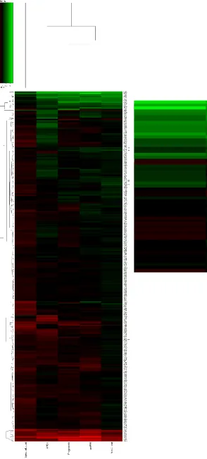
A straightforward method was sought to compare the results from the different software packages in order to assess whether there was a consensus in the data. A consensus between packages would make it possible to test the hypothesis that the consensus results will give a better measure of differential expression than any single package alone. This hypothesis follows the logic behind improving sensitivity in peptide/protein identification through the use of multiple search engines[3, 104], and extends it to quantitative analyses. The methods chosen to investigate this hypothesis were heatmaps of the data, and ROC plots generated using the QPROT Z-statistic. Both the heatmaps and the the pseudo-ROC plots were generated using the R statistical package.

2.3.9.1 - Heatmap generation

Log10 ratios were calculated between the E/B, E/C and E/D conditions and the maps

2.3.9.2 - QPROT Z-statistic

This method of comparison used the more stringent thresholds detailed above in 2.3.6.2. The Z-statistic itself is a measure of the distance (in standard deviations) from the mean in normally distributed data. The QPROT tool analyses the global distribution of the data from each software package and thus multiple Z-statistic values are broadly comparable across the different packages. If a given protein had not been measured by a particular package, the Z-statistic for that package was scored as zero to denote that there was no evidence for differential expression.

As the statistic values are comparable across packages, the absolute value of the mean Z-statistic was taken in order to combine the results from the four software packages, bringing all data onto the same scale as the absolute value is an approximation of the global strength of differential expression (either up or down) as calculated by each of the different packages. These values were also plotted on the pseudo-ROC plots to assess this combination method as a way to improve sensitivity with respect to the plots from each individual package.

2.4 - Results

2.4.1 – ABRF data

We analysed the ABRF data set (yellow/red comparison) to see how well the different software packages agreed. First we looked at the proteins that were scored as significantly changing (p<0.05) by each of the software pipelines and were contained within the answer key. Across the different pipelines, over 500 proteins were scored as significantly changing, with only 22 proteins being common across all pipelines, thus showing the general

[image:58.595.136.431.73.726.2]

Following the analysis of those heatmaps generated from the ABRF dataset it was concluded that the setup was too artificial, and as the true real answer is unknown it is impossible to draw any conclusions about software quality based on the analysis of this dataset with any confidence. As such further stages of analysis were not completed for this dataset.

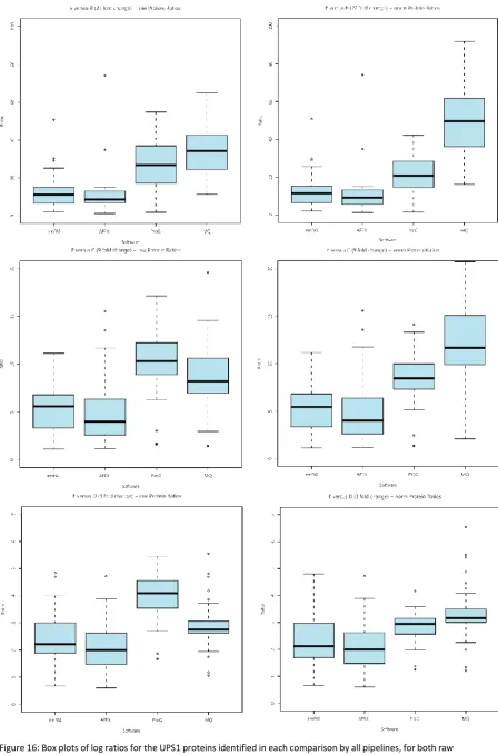
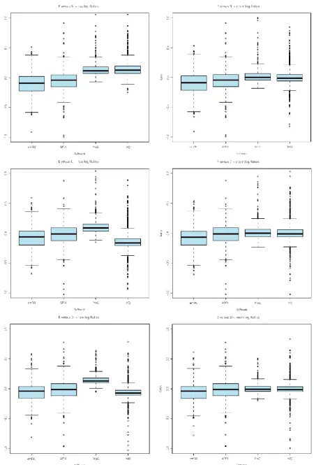
2.4.2 - CPTAC ratio calculation

Ratios were calculated for the spiked in UPS proteins in the CPTAC dataset to compare the experimental ratios with the known ratios between the spike-in amounts for the E/B (27 fold change), E/C (9 fold change) and E/D (3 fold change) comparisons, using the four software pipelines: emPAI, APEX, Progenesis LC-MS and MaxQuant. It was observed (see Figure 16) that the two intensity based pipelines gave greater accuracy as measured by the median protein ratios. Progenesis LC-MS gives the closest median ratio values to those expected from this dataset, 26.8, 10.3 and 4.1 for raw values and 20.8, 8.5 and 3.0 after normalisation with the expected values being 27,9 and 3. MaxQuant also produced relatively accurate ratios in the raw data, 34.2, 8.2 and 2.7, but this time normalisation appears to increase the ratios, to 49.6, 11.7 and 3.2. Both intensity-based packages produce similar values for the interquartile range of the data. This indicates that the relative spike-in has been done correctly across the different samples; however there are inherent differences in the abundances of proteins present in the yeast background. Differences in the yeast background can also be observed in box plots of the yeast log ratios before and after normalisation for each package.