Causality in real-time dynamic substructure testing

This is a repository copy of Causality in real-time dynamic substructure testing. White Rose Research Online URL for this paper:

http://eprints.whiterose.ac.uk/79709/ Version: Submitted Version

Article:

Gawthrop, P.J., Neild, S.A., Gonzalez-Buelga, A. et al. (1 more author) (2009) Causality in real-time dynamic substructure testing. Mechatronics, 19 (7). 1105 - 1115. ISSN

0957-4158

https://doi.org/10.1016/j.mechatronics.2008.02.005

Reuse

Unless indicated otherwise, fulltext items are protected by copyright with all rights reserved. The copyright exception in section 29 of the Copyright, Designs and Patents Act 1988 allows the making of a single copy solely for the purpose of non-commercial research or private study within the limits of fair dealing. The publisher or other rights-holder may allow further reproduction and re-use of this version - refer to the White Rose Research Online record for this item. Where records identify the publisher as the copyright holder, users can verify any specific terms of use on the publisher’s website.

Takedown

If you consider content in White Rose Research Online to be in breach of UK law, please notify us by

Causality in real-time dynamic substructure testing

P.J. Gawthrop

S.A. Neild

A. Gonzalez-Buelga

D.J. Wagg

a_{Centre for Systems and Control and Department of Mechanical Engineering, University}

of Glasgow, GLASGOW. G12 8QQ Scotland.

b_{Department of Mechanical Engineering, Queens Building, University of Bristol, Bristol}

BS8 1TR, UK.

Abstract

Causality, in the bond graph sense, is shown to provide a conceptual framework for the design of real-time dynamic substructure testing experiments. In particular, known stabil-ity problems with split-inertia substructured systems are reinterpreted as causalstabil-ity issues within the new conceptual framework.

As an example, causality analysis is used to provide a practical solution to a split-inertia substructuring problem and the solution is experimentally verified.

Key words: Substructuring; hardware-in-loop testing; causality; bond graphs.

1 Introduction

Real-time dynamic substructure testing is a hybrid numerical-experimental test-ing technique for simulattest-ing the dynamics of structures. It allows critical elements within a structure to be experimentally tested at full scale, whilst subjected to dy-namic forcing. The structure under consideration is split into an experimental test piece (or physical substructure) and a numerical model describing the remainder of the structure (or numerical substructure). The challenge is to ensure that the phys-ical and numerphys-ical substructures interact in real-time such that they emulate the behaviour of the complete structure during dynamic excitation.

Hybrid testing of large civil engineering structures subjected to extreme dynamic loading, such as earthquakes, has been successfully performed for many years at ex-panded time-scales (known as pseudo-dynamic testing [1–4]). For large structures,

a significant advantage of substructuring is that scaling effects can be eliminated as the portion of the structure being tested physically can be at full-scale. Due to the quasi-static nature of these expanded time-scale tests, a limitation is that dy-namic and hysteretic forces must be estimated. Real-time tests, which allow the experimental testing of velocity-dependent characteristics, were first proposed by Nakashima et.al. [5]. Current real-time substructuring research falls broadly into two main areas; the development of numerical integration algorithms to compute the numerical model [6–8] and the development of control strategies to at the inter-face between the two substructures [9–12]. This paper is motivated from the control engineering approach, but has implications which span both areas of work. This is because the causality of a real-time dynamic substructure test is largely indepen-dent of both the control and numerical integration methods used. The causality is a property of how the two systems are joined, and where the division between numer-ical and physnumer-ical is chosen. For many systems causal conflict can occur, with the result that the system can be unstable and/or un-implementable. By using a simple example, we seek to explain how causality in real-time dynamic substructuring is an essential concept which should be used in the design of all such tests.

Analysis of the system causality can be done in a number of ways. In this work the motivation comes from bond graphs [13–17], for which analytical and numerical methods for analysing causality have been established. Bond graph analysis has already been applied to real-time dynamic substructuring by Gawthrop, Wallace & Wagg [18], where the concept of a virtual junction between numerical and physical subsystems was developed. A introduction to causality and bond graphs is given by Gawthrop & Bevan [17] and an in-depth discussion of causality is given by Marquis-Favre & Scavarda [19]; In substructuring there are three main issues which relate to causality:

(1) The inclusion or exclusion of inertia, damping or elastic forces in either sub-system can affect the causality of the substructured model.

(2) The form of the numerical model will be determined by the causality substruc-tured model. Ideally an ordinary differential equation form is sought rather than a differential-algebraic equation which is more difficult to implement nu-merically.

(3) The design of the transfer system (described in detail below), in particular the choice of force or displacement actuation, depends on the causality of the substructured model.

In some situations it is possible to have causal conflict which in substructuring usually indicates problems relating to items 1–3.

diagrams may be more familiar, results are interpreted in this way thoughout the paper. However, the bond graph approach is more general as it encompasses non-linear and multivariable systems as well; more importantly, although the block di-agram is a useful way of presenting bond graph results, the results could not have been obtained as easily using block diagrams alone.

Substructuring involving split-mass systems is known to give rise to implemen-tation problems [12, 20]. This paper provides a new causality-based conceptual framework for such systems as well as an experimentally-verified practical solu-tion.

The purpose of this paper is to explain why causality is an important issue for real-time dynamic substructuring. Section 2.1 gives a causality-based framework for substructuring and gives illustrative examples. Section 4 focuses on situations where there is causal conflict and proposes a solution based on the design of a

coupling system. Section 5 applies the methods to an experimental coupled

pendu-lum oscillator system [20,21]; the range of experimental parameters is substantially increased using the new approach. Section 6 concludes the paper.

2 Substructuring and Causality

2.1 Substructuring

The physical and numerical substructures interact through the application of inter-face equilibrium and compatibility conditions. This may be achieved by measuring the force at the interface and imposing it on the numerical substructure within the numerical integration routine, hence satisfying the equilibrium condition. Then the interface displacement computed from the numerical model is imposed on the phys-ical system, satisfiying the compatibility condition. A transfer system (typphys-ically an actuator) is required to impose the interface displacement calculated from the nu-merical substructure on the physical substructure. We refer to this substructuring configuration as flow actuation (adopting the bond graph terminology in which in-teractions between systems are thought of as efforts and flows). Alternatively, the measured interface displacement may be imposed on the numerical substructure and the resulting computed force imposed on the physical system. This configura-tion, in which the transfer system is required to impose the interface force, we term

effort actuation.

a single electric or hydraulic actuator but may be more complex, for example an hydraulic shaking table [12]. Typically the actuator has an in-built or ‘proprietary’ controller, which is usually some form of PID control, and would provide a suf-ficient level of control for standard dynamic testing. However, in substructuring, there is a second feedback loop through the numerical model in addition to the controller feedback loop. The implication of the second feedback loop is that the control accuracy required for real-time substructuring is far greater than for stan-dard dynamic testing. It is now well established that the proprietary controller is not sufficient to compensate for the actuator dynamics, particularly when testing lightly damped structures such as those typically found in civil engineering [7, 22, 23]. To reduce the effect of actuator dynamics, a range of control strategies which can be implemented as an outer-loop around the proprietary (inner-loop) controller have been proposed [10–12, 18, 22]. Gawthrop et.al [24] presented a technique to calcu-late the required control accuracy in terms of the maximum transfer system delay before system instability occurs. It has been observed that for lightly damped sys-tems representative of those found in civil engineering this delay can be less than 1 ms [7].

For simplicity, we will assume that the transfer-system dynamics are linear and given by the transfer function Te(s)in the case of effort actuation and Tf(s)in the

case of flow actuation. As discussed previously [24], it is convenient to approximate these dynamics by a pure time-delay for the purposes of design.

2.2 Causal analysis of the ideal case

For a substructuring test where the compatibility condition is imposed on the phys-ical substructure the actuator will need to be in displacement control and hence have a displacement feedback loop. In this case the equilibrium condition must be imposed on the numerical substructure and to achieve this the actuator force is measured and fed into the numerical substructure which in turn generates the dis-placement demand for the actuator – hence closing the second feedback loop. This combination of equilibrium and compatibility conditions ensures that the system is

causal. It is possible to swap the conditions between the two subsystems, and still

retain a causal system. However, it is also possible to propose a range of non-causal substructuring configurations. So the first observation we make is that a causal sub-structuring system arises naturally when a ‘collocated’ equilibrium-compatibility condition is used.

[Fig. 1 about here.]

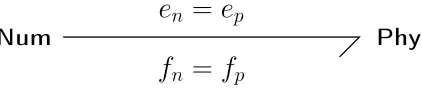
To formalise this concept we consider the bond graph shown in Figure 1 which shows a substructured system where Numand Phyrepresent the numerical and

bond graph representation and are joined by a single bond representing the ideal coupling of the two subsystems (i.e. ignoring transfer system effects). Interactions between elements within a bond graph are defined in terms of an effort (which in this case is force) and flow (the bond graph convention is to use velocity however we will use displacement as this relates to our later analysis). In Figure 1, endenotes

the numerical effort (force) and ep the physical effort (force). Similarly the flows

(displacements) are denoted fnand fpcorresponding to the numerical and physical

displacements respectively. In the ideal substructuring case en=epand fp= fn, as

denoted by the bond graph in Figure 1 [24]. In fact the bond graph formalises the concept of a collocated equilibrium-compatibility condition exactly by the effort and flow conditions defined on the bond. So the bond graph in Figure 1 represents the coupling of the two subsystemsNumandPhyusing the equilibrium condition

en=epand the compatibility condition fp= fn. There are two causality cases for

the substructured system in Figure 1 corresponding to using either effort or flow actuation.

2.3 Choosing effort or flow actuation

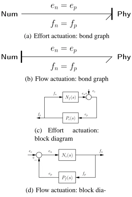
The ideal case shown in Figure 1 ignores the transfer system but is useful to demon-strate the difference in causality between force (effort) and displacement (flow) actuation. This is shown in Figure 2 in both bond graph and block diagram form.

[Fig. 2 about here.]

Figure 2(a) shows the bond graph for effort (force) actuation and Figure 2(b) shows the case for flow actuation (displacement control). The two causality cases are dis-tinguishable by the causal stroke (the vertical line drawn at one end of the bond) which indicates whether effort or flow is imposed on the subsystems joined by the bond — see [17] for further details. Each case can also be represented as a block-diagram representation. The block block-diagram of Figure 2(c) corresponds to Figure 2(a) and Figure 2(d) corresponds to Figure 2(b). In the block diagrams we have introduced transfer function representations ofNumandPhywhich are N(s)and

P(s)respectively, where s is a complex scalar i.e. the Laplace domain variable. The subscripts e and f are used to denote whether the transfer functions N(s)and P(s) are defined for effort of flow causality respectively. It is important to note that the physical substructure (Phy) is typically strongly nonlinear and so a transfer func-tion representafunc-tion is not normally possible. However, it is useful in this context to analyse the closed loop system with (Phy) approximated by P(s) +f(·), where

f(·) represents the some arbitrary nonlinear dynamics which will be neglected, without loss of generality, in some of our analysis.

by Gawthrop & Bevan [17]). In fact the relationship can be expressed as

Nf(s) =Ne−1(s), (1)

Pf(s) =Pe−1(s). (2)

As a result if the transfer functions are strictly proper (i.e. with relative degree≥1) in one configuration then they will be improper in the other. In the later case causal conflict can occur, or the system could be non-causal. The examples shown later demonstrate that this causal conflict often manifests itself as a change from integral to derivative causality. A discussion on the problems associated with derivative causality can be found in [17].

2.4 Natural causality

In bond graph terms the natural causality of a system is that where the dynamic bond graph components I(representing masses) andC(representing springs) are in integral causality [17]: the block diagram equivalent is an integrator rather than a differentiator. In this case, the corresponding system transfer function is proper. In the sequel, we associate the proper transfer function P(s) with Phyin natural causality and the proper transfer function N(s)withNumin natural causality.

Implementing the system in it’s natural causality will minimise problems associated with points 1– 3 and should be seen as an important part of preliminary substruc-turing design. The concept of natural causality (as we use it here) is not formalised beyond the conceptual, and we note that example systems can be configured in which natural causality either does not exist or alternatively is non-unique.

Defining a natural causality depends primarily on the definition of the substructur-ing problem, which includes point 1; the inclusion or exclusion of inertia, dampsubstructur-ing or elastic forces in either subsystem. In some cases, when defining the substructur-ing problem, there is a choice of how the system can be divided/coupled, and in this situation causality analysis can be used as a tool to ensure the system has a natural causality.

differential-algebraic equation solver is not required. This resolves the issue raised in point 2.

3 Dividing the system: A mass-spring-damper example

The choice of which parts of the complete system are to form Phyand Numis often dictated by practical issues such as which particular component of the overall system needs to be tested. Beyond this there may be some flexibility in (i) choos-ing where to divide the system, and (ii) chooschoos-ing whether to split a component between the substructures. In this section we consider a linear mass-spring-damper system which demonstrates the key concepts associated with the dividing/coupling process.

[Fig. 3 about here.]

[Table 1 about here.]

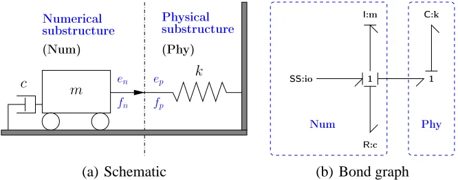
The mass-spring-damper system can be divided in a number of ways, and in Figure 3 the case is shown wherePhycontains the spring and the numerical substructure Numcontains the mass and damper. This division is shown schematically in Fig-ure 3(a) and the corresponding bond graph is shown in FigFig-ure 3(b). The natural causality can be found either by using the bond graph, Figure 3(b), (using SCAP) or by examining the transfer functions. In this case the divided system corresponds to the causality of Figure 2(b) which corresponds to flow (i.e. displacement) actua-tion. This corresponds directly to the block diagram shown in Figure 2(d) and the transfer functions Pf and Nf are defined in the first row of Table 1 — see Gawthrop,

Wallace & Wagg [18] for a more complete discussion of this system.

3.1 Splitting components

In this section we consider the consequences of splitting the spring betweenNumand Phy. This is achieved by using the parameter αto indicate the proportion of the component placed inNum. Having considered the case for splitting the spring we repeat the process for the damper and the mass.

in the feedback loop respectively:

Le(s) =Ne(s)Pe(s) (3)

Lf(s) =Nf(s)Pf(s) (4)

The loop gain and phase margin will be used for comparing cases for differentα values.

3.1.1 Split spring

[Fig. 4 about here.]

[Table 2 about here.]

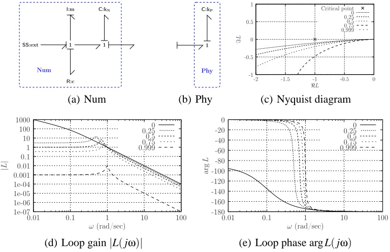
The case for the split spring is shown in Figure 4. The bond graphs in Figures 4(a) & 4(b), now indicate that the spring is divided in two parts, one inNumand the other inPhy. This system retains the original (integral) causality of the case when all the spring was in Phy. The corresponding transfer functions Nf(s) and Pf(s)

(in the second row of Table 1) are proper.

The frequency response of the loop gain Lf(s)(given by equation (4)) is shown in

two forms. The Nyquist diagram shown in Figure 4(c) shows that stability margin increases with increasing α. This is expected, because when α=1 the system is entirely numerical, with no physical component, and so it will no longer be a sub-structured system. The modulus of the frequency response is shown in Figure 4(d), with the corresponding phase shown in Figure 4(e). This shows that the loop-gain goes to zero at high frequencies, indicating that high frequencies are attenuated. The phase marginsφmmeasured from these plots give an indication of how robust

the system is to delay (and other uncertainties) in the transfer system (as discussed in [24]). The variation of phase margin is shown in Figure 4(e) and summarised in Table 2 . As shown by the Nyquist diagram, the stability (i.e. phase) margin increases with increasingα.

3.1.2 Split damper

[Fig. 5 about here.]

[Table 3 about here.]

3.1.3 Split mass

[Fig. 6 about here.]

[Table 4 about here.]

The split mass case is shown in Figure 6. This case is significantly different from the previous two cases. In this case the causality has changed from integral to deriva-tive. This can be ascertained either from the bond graphs shown in Figures 6(a) & 6(b), or the transfer functions shown in (Table 1). Specifically, the physical part of the mass has derivative causality and Pf(s)is improper.

As before the frequency response of the loop gain Lf(s)is shown as both a Nyquist

diagram, Figure 6(c) and as loop gain, Figure 6(d) and phase margin, Figure 6(e). The Nyquist diagram shows that stability margin increases with α. However, the loop gain shows that at high frequencies Lf(s)does not go to zero but rather that

Lf(∞) = ₁₋α_α. Thus ifα>0.5, the phase margins, shown in Figure 6(e) reduce to

zero and the system becomes unstable for an arbitrarily small phase delay in the transfer system.

In this discussion, flow actuation has been considered. In the case of the split-mass, switching to effort actuation does not resolve the restriction onα. From equations (1), (2), (3) and (4), it can be seen that the loop gain in effort actuation Le(s)is the

inverse of the loop gain in flow actuation. Therefore, as with flow actuation, at high frequencies the loop gain does not tend to zero, resulting in the condition that if α<0.5 a small delay would induce instability. From a causality viewpoint, in the case of flow actuation the Phytransfer function is non-proper and in the case of effort actuation theNumtransfer function is non-proper.

An approach to resolving this causal conflict is given in the next section.

4 System design to avoid causal conflict

[Fig. 7 about here.]

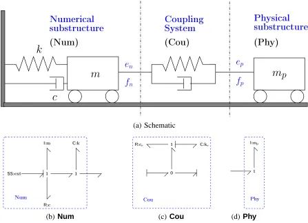
In general,Couis a two-port (and therefore two-input, two-output) system which, in the linear case would have four scalar transfer functions to describe it. Figures 7(b) and 7(c) give two simple special cases ofCouwhich, in the linear case, are as-sociated with the single transfer function corresponding to the one-port subsystem cou. With the causality given, the version of Figure 7(b) imposes effort on both ports whereas the version of Figure 7(c) imposes flow on both ports. As discussed in Section 4.1,coucould, for example, represent a damped spring.

Figure 7(d) gives the block diagram corresponding to the bond graph of Figure 7(a) when using the version ofCougiven in Figure 7(b) and, as discussed in Section 3, where N(s), C(s) and P(s) are the transfer functions corresponding to Num, couandPhyin natural causality.

[Fig. 8 about here.]

[Fig. 9 about here.]

A key observation is that Figure 7(d) shows two loops and there are, therefore, two loop gains. As discussed in Section 2.1, the loop gain is important when analysing robust stability of the substructured system. The question arises as to which loop is the relevant one in this case. As discussed previously [18, 24], it is the transfer

sys-tem, providing the interface between numerical and physical substructures, which

causes stability problems. Therefore it is the location of the transfer systemTra that determines the critical loop to consider. The two possibilities correspond to whether the transfer system generates flow or effort and lead to Figures 8 and 9 respectively. In each of these figures, (a) gives the bond graph of the substructured system with Traincluded but without Cou, (b) gives the bond graph with Couincluded and (c) and (d) give the corresponding block diagrams. We can now write down the expressions for the loop gain and the closed-loop frequency response (D) as

Lf =

N

P Df =

NP

N+P (5)

Le=

P

N De=Df (6)

Lp=

CN

1+CP Dp=

N(1+CP)

1+C(N+P) (7)

Ln=

CP

1+CN Dn=Dp (8)

(9)

Note that at those frequenciesωwhere C(jω)is large:

Ln(jω)≈Lf(jω) (10)

Lp(jω)≈Le(jω) (11)

In the case of Figure 7(b):

ep=en=Ce(s)(fn−fp) (13)

and in the case of Figure 7(c):

fp= fn=Cf(s)(en−ep) (14)

where Ce(s)and Cf(s)are the transfer functions corresponding to couwith effort

and flow output respectively.

4.1 Example: Split mass system

[Fig. 10 about here.]

Split-mass systems are common in substructuring – see,for example, Neild et. al. [12]. The system used as an example in this section is a linearised version of a coupled oscillator-pendulum system which has been analysed previously [20, 21]; new experimental results appear in Section 5 of this paper. In particular, it was shown [21] that a key parameter is the ratio p of the two masses (p= mp

m) and

that stable substructuring requires p<1. As will be shown in Section 4.1.1, this result is a direct consequence of causal conflict. With natural causality, the transfer functions corresponding toNum,couandPhyrespectively are:

N(s) = s

ms2_+cs_+k (15)

C(s) = ccs+kc

s (16)

P(s) = 1

mps

= 1

pms (17)

The following subsections correspond to the bond graphs displayed in Figures 8(b) and 9(b) (with the block diagram equivalents of Figures 8(d) and 9(d) using the special coupling systemCouof Figure 7(b).

4.1.1 Flow actuation

[Fig. 11 about here.]

With reference to Figure 8(a), withoutCou, there is causal conflict; eitherNumor Phy, but not both, has natural causality. With flow actuation, this leads to a loop gain given by (5)

Lf(s) =

N

P =

pms2

Setting s= jωand lettingω→∞, it follows that this loop gain has a constant high-frequency gain of p. Following the standard textbooks, this high-high-frequency gain must be less than unity for stability. This corresponds to the result of Gonzalez-Buelga et. al. [21]. Note that in the paper of Neild et. al. [12], p= 20

100 =0.2.

However, from (7), insertingCougives the loop gain:

Lp=

CN

1+CP =

mps2(ccs+kc)

(mps2+ccs+kc)(ms2+cs+k)

(19)

As Lp is proper, limw→∞Lp(jω) =0: the high-frequency gain is zero. This

im-plementation implies that the transfer system Traimposes flow onto the physical system; it must implement a form of displacement control.

In view of (19), it is convenient to reparameterise Couin terms of natural fre-quencyωcand damping ratioξcwhen coupled toPhy:

kc=mpω2c (20)

cc=2mpξcωc (21)

The implication of includingCouinPhyis that a physical spring must be attached between the physical mass mpand the actuator. This idea has been previously

sug-gested by [11].

[Fig. 12 about here.]

Alternatively, using elementary block-diagram manipulation on Figure 8(d), it fol-lows that

ep=

C(s)Tf(s)

1+C(s)P(s)fn=P

−1_(s)T

f(s)

C(s)P(s)

1+C(s)P(s)fn (22)

The latter form of the equation corresponds to Figure 12 and can thus be imple-mented numerically. In particular, using (16) and (17), the required filter is:

C(s)P(s) 1+C(s)P(s) =

ccs+ks

mps2+ccs+ks

(23)

However, this formulation is based on the assumption that Phyis linear with a known transfer function P(s). If these assumptions do not hold then the implemen-tation of Figure 12 is an approximation to the implemenimplemen-tation of Figure 8(d).

4.1.2 Effort actuation

The use of flow actuation (Section 4.1.1) leads to either the physical implementa-tion of the coupling systemCouor an approximate numerical implementation. An alternative approach is to use effort actuation and implementCounumerically.

With reference to Figure 9(a), withoutCou, there is causal conflict; eitherNumor Phy, but not both, has natural causality. With effort actuation, this leads to a loop gain given by (6)

Le(s) =

P

N =L

−1

f (s) =

ms2+cs+k

pms2 (24)

This loop gain has a constant high-frequency gain of 1_p. Once again, this con-stant high-frequency gain is undesirable; however, from (8), inserting Cougives the loop gain:

Ln=

CP

1+CN =

(ccs+kc)(ms2+cs+k)

mps2(ms2+ (c+cs)s+ (k+kc))

(25)

As Lnis proper, limw→∞Ln(jω) =0: the high-frequency gain is zero.

This implementation implies that the transfer system Traimposes effort onto the physical system; it must implement a form of force control.

With reference to Figure 9(d), the force control represented by the transfer sys-tem Tf(s)is embedded within a feedback loop involving P(s)and C(s). In control

system terms, Te(s)represents an inner-loop, C(s)a controller and P(s)a system.

The interpretation of the bond graph representing C(s) as a controller is explored in [17, Figure 11].

5 Experimental Results

[Fig. 14 about here.]

The experimental system is shown in Figure 14. This system has been discussed previously [20, 21] and analysed in terms of its equations of motion linearised about the vertical down pendulum position. As the purpose of the experiment is to examine non-linear system behaviour for a range of parameters, it is advantage to have as wide range of parameters as possible. A key parameter is the mass ratio

[Fig. 15 about here.]

In this section, a redesign of the substructuring experiment based on the causality reasoning of Section 4.1 will allow the range of parameter p to be increased to include values of p>1. As in the previous work, this analysis is based on a lin-earised system model and results presented in this section show experimentally that the predicted enhanced parameter range is experimentally feasible when applied to the actual non-linear system.

The experimental setup used was the same as that reported by [21] except that the coupling system Couis included in the form of (23) of Section 4.1.1. The excitation to the system is via a force Fe=αsin(ωet), acting on the

mass-spring-damper system. See figure 14. Two different sets of experiments were developed: in the first ones we show that it is possible to conduct substructuring tests when

p>1. In the second ones we study their accuracy. As in [21], it is useful to express results in terms of the effective delayτleading to instability. In particular we define

τc=

φm

ωm

(26)

whereφmis the phase margin andωmthe corresponding frequency, such thatτc

rep-resents the critical delay value at which the system goes unstable. This phenom-ena has been demonstrated using experimental substructuring tests, for example in [21, Figure 6], where experimental and theoretical results showing the stability boundary of the substructured relating p=_Mm to delayτare shown.

Previous experiments had shown that the actuator had an effective delay of τa =

0.025sec. In order to locate the stability boundary an additional variable numerical delay,τnwas added during the tests. Different p ratios where tested by changing the

pendulum bob (m). For each value of p shown in Figure 15, the delayτ=τa+τn

was increased until the onset of instability at τ=τc. Results for two different ωc

values are shown in Figure 15. As can be seen from Figure 15(a), an experimental value of p=1.65 was reached. For comparison, the highest experimental value re-ported in [21, Figure 6.] was about p=0.6. Because of the built in actuator delay (τa=0.025sec), it was not possible to reduceτfurther than shown. It’s important to

note that, despite the limitations of the experiment, the theoretical curve becomes asymptotic to the p axis as p→∞, whereas without the coupling system the curve terminates at the p=1 point [20, 21]. So the effect of introducing the coupling sys-tem in this case is (i) to increase the stable zone of operation for the substructuring system, and (ii) to allow the p>1 case to be simulated.

In the second set of experimental hybrid tests, to highlight the significance of the improvement achieved, we have performed experimental substructuring simula-tions of the stability boundary of the semitrivial solution (the downward vertical position of the pendulum is stable) in the α−ωˆ parameter space. αis the magni-tude of the external excitation and ˆω= ωe

frequency and twice the pendulum frequency.

The stability boundary marked ‘Theory’ in Figure 16 corresponds to a line of sub-critical Hopf bifurcations. Above this line the downward vertical pendulum position becomes unstable [26]. In the previous work, [21], this was carried out for p=0.1, and p=1 was not possible. The results shown in Figure 16 are produced using the coupling system with p=1.

[Fig. 16 about here.]

A clear resonance can be seen at ˆω=1, with the stable zone being below the data lines. There is a good correlation between experimental substructuring results and the theoretical curve.

6 Conclusion

Building on the bond graph framework of Gawthrop et. al. [18], the causality at-tribute of the bond graph approach has been used to examine issues of substruc-turing arising when components are split between the numerical and physical sub-strucures. The concept of a coupling system has been introduced and shown to overcome problems arising when a mass is split. A set of experiments reported by Gonzalez-Buelga et. al. [21] is redesigned using the coupling system concept and rerun with parameter values not previously compatible with stability of the sub-structured system.

References

[1] F. Molina, S. Sorace, G. Terenzi, G. Magonette, B. Viaccoz, Seismic tests on reinforced concrete and steel frames retrofitted with dissipative braces, Earthquake Engng Struc. Dyn. 33 (2004) 1373–1394.

[2] P. Shing, S. Mahin, Seismic tests on reinforced concrete and steel frames retrofitted with dissipative braces, Earthquake Engng Struc. Dyn. 15 (1987) 409–424.

[3] J. Donea, G. Magonette, P. Negro, P. Pegon, A. Pinto, G. Verzeletti, Pseudodynamic capabilities of the elsa laboratory for earthquake testing of large structures., Earthquake Spectra 12 (1996) 163–180.

[4] O. Bursi, P. Shing, Evaluation of some implicit time-stepping algorithms for pseudodynamic tests, Earthquake Engng Struc. Dyn. 25 (1996) 333–355.

[6] A. Blakeborough, M. Williams, A. Darby, D. Williams, The development of real-time substructure testing., Philosophical Transactions of the Royal Society pt. A 359 (1869-1891).

[7] P. Bonnet, C. Lim, M. Williams, A. Blakeborough, S. Neild, D. Stoten, C. Taylor., Real-time hybrid experiments with newmark integration, mcsmd outer-loop control and multi-tasking strategies, Earthquake Engng Struc. Dyn. 36 (2007) 119–141.

[8] O. Bursi, A. Gonzalez-Buelga, S. Neild, L. Vulcan, D. Wagg, Novel partitioned rosenbrock-based algorithms for real-time dynamic substructure testing, Earthquake Engng Struc. Dyn. xx (2007) xx.

[9] A. P. Darby, A. Blakeborough, M. S. Williams, Improved control algorithm for real-time substructure testing, Earthquake Engng Struc. Dyn. 30 (3) (2001) 431–448.

[10] M. Wallace, J. Sieber, S. Neild, D. Wagg, B. Krauskopf, A delay differential equation approach to real-time dynamic substructuring, Earthquake Engng Struc. Dyn. 34 (15) (2005) 1817 – 1832.

[11] A. Reinhorn, M. Sivaselvan, Z. Liang, X. Shao, Real-time dynamic hybrid testing of structural systems., in: Thirteenth World Conference on Earthquake Engineering, Vancouver, 2004, paper No 1644.

[12] S. Neild, D. Stoten, D.Drury, D.J.Wagg, Control issues relating to real-time substructuring experiments using a shaking table, Earthquake Engng Struc. Dyn. 34 (2005) 1171–1192.

[13] F. E. Cellier, Continuous system modelling, Springer-Verlag, 1991.

[14] P. J. Gawthrop, L. P. S. Smith, Metamodelling: Bond Graphs and Dynamic Systems, Prentice Hall, Hemel Hempstead, Herts, England., 1996.

[15] D. Karnopp, D. L. Margolis, R. C. Rosenberg, System Dynamics : Modeling and Simulation of Mechatronic Systems, 3rd Edition, Horizon Publishers and Distributors Inc, 2000.

[16] A. Mukherjee, R. Karmakar, A. Samantaray, Bond Graph in Modeling, Simulation and Fault Detection, I.K. International Publishing, New Delhi, 2006.

[17] P. J. Gawthrop, G. P. Bevan, Bond-graph modeling: A tutorial introduction for control engineers, IEEE Control Systems Magazine 27 (2) (2007) 24–45.

[18] P. Gawthrop, M. Wallace, D. Wagg, Bond-graph based substructuring of dynamical systems, Earthquake Engng Struc. Dyn. 34 (6) (2005) 687–703.

[19] W. Marquis-Favre, S. Scavarda, Alternative causality assignment procedures in bond graph for mechanical systems, Journal of Dynamic Systems, Measurement and Control, Transactions of the ASME 124 (2002) 457–463.

[21] A. Gonzalez-Buelga, D. Wagg, S. A. Neild, Parametric variation of a coupled pendulum-oscillator system using real-time dynamic substructuring, Structural Control and Health Monitoring xx (xx) (2007) xx, published on-line 17 Oct 2006.

[22] A. Darby, M. Williams, A. Blakeborough, Stability and delay compensation for real-time substructure testing, ASCE Journal of Engineering Mechanics 128 (2002) 1276– 1284.

[23] C. Lim, S. Neild, D. Stoten, D. Drury, C. Taylor, Adaptive control strategy for dynamic substructuring tests, ASCE Journal of Engineering Mechanics xx (2007) xx.

[24] P. Gawthrop, M. Wallace, S. Neild, D. Wagg, Robust real-time substructuring techniques for under-damped systems, Structural Control and Health Monitoring 14 (4) (2007) 591–608, published on-line: 19 May 2006.

[25] G. Goodwin, S. Graebe, M. Salgado, Control System Design, Prentice Hall, 2001.

List of Figures

1 Bond graph interpretation of substructuring 19

2 Bond graph Causality. 20

3 A mass-spring-damper system. 21

4 Split spring 22

5 Split damper 23

6 Split mass 24

7 Avoiding causal conflict using a coupling systemCou 25

8 Coupling system: flow actuation 26

9 Coupling system: effort actuation 27

10 Split-mass system. 28

11 Frequency responses: flow actuation 29

12 Approximate numerical implementation 30

13 Frequency responses: effort actuation 31

14 Experimental Pendulum-Oscillator System 32

15 Experimental results. (a),(b) give experimental measurements of the onset of instability compared with theoretical values for the linear case this corresponds to [21, Fig. 6] but with larger

mass-ratio p. 33

e

=

e

f

=

f

Num Phy

Fig. 1. Bond graph interpretation of substructuring.Numis the numerical substructure (im-plemented in software) andPhyis the physical substructure. The bond linkingNumand

e

=

e

f

=

f

Num Phy

(a) Effort actuation: bond graph

e

=

e

f

=

f

Num Phy

(b) Flow actuation: bond graph

Pe(s)

Nf(s)

ep

fn

fp

−

+

en

ee

(c) Effort actuation: block diagram

Pf(s)

Ne(s)

ee fn

fp

ep

en +₋

(d) Flow actuation: block dia-gram

Fig. 2. Bond graph Causality. (a) The causal stroke indicates that effort is imposed on

Phyand flow is imposed on Num; this corresponds to force actuation. (b) The causal stroke indicates that flow is imposed onPhyand effort is imposed onNum; this corre-sponds to position actuation. (c) The block diagram corresponding to the bond graph of (a). (d) The block diagram corresponding to the bond graph of (b). Note that Ne=N−f1and

Pe=P−_f 1. In (c) and (d) an external effort has been added for later use corresponding to an

Numerial substruture

(Num)

Physial substruture

(Phy)

en

fn

ep

fp

m

c k

(a) Schematic

Num Phy

1 1

R:c

I:m C:k

SS :io

(b) Bond graph

Num

1 1

R:c

I:m C:k_N

SS:[out℄ SS:ext (a) Num Phy 1 C:kP SS:[in℄ (b) Phy -1 -0.5 0 0.5

-2 -1.5 -1 -0.5 0

ℑ L ℜL Critialpoint 0 0.25 0.5 0.75 0.999

(c) Nyquist diagram

1e-07 1e-06 1e-05 1e-04 0.001 0.01 0.1 1 10 100 1000

0.01 0.1 1 10 100

| L | ω(rad/se) 0 0.25 0.5 0.75 0.999

(d) Loop gain|L(jω)|

-180 -160 -140 -120 -100 -80 -60 -40 -20 0

0.01 0.1 1 10 100

ar g L ω(rad/se) 0 0.25 0.5 0.75 0.999

(e) Loop phase arg L(jω)

Fig. 4. Split spring: kN=αk, kP= (1−α)k, k=m=1, c=0.1. Unlike Figure 3, the spring

Num

1

R:c_N I:m SS :[out℄ SS:ext (a) Num Phy 1

R:c_P C:k SS:[in℄ (b) Phy -1 -0.5 0 0.5

-2 -1.5 -1 -0.5 0

ℑ L ℜL Critialpoint 0 0.25 0.5 0.75 0.999

(c) Nyquist diagram

1e-05 1e-04 0.001 0.01 0.1 1 10 100 1000 10000

0.01 0.1 1 10 100

| L | ω(rad/se) 0 0.25 0.5 0.75 0.999

(d) Loop gain|L(jω)|

-180 -170 -160 -150 -140 -130 -120 -110 -100 -90

0.01 0.1 1 10 100

ar g L ω(rad/se) 0 0.25 0.5 0.75 0.999

(e) Loop phase arg L(jω)

Fig. 5. Split damper: cN = (1−α)c, cP=αc, k=m=1, c=0.1. Unlike Figure 3, the

Num

1

R:c I:mN

SS :[out℄

SS:ext

(a) Num

Phy

1

I:m_P C:k SS:[in℄ (b) Phy -1 -0.5 0 0.5

-2 -1.5 -1 -0.5 0

ℑ L ℜL Critialpoint 0 0.25 0.5 0.75 0.999

(c) Nyquist diagram

1e-05 1e-04 0.001 0.01 0.1 1 10 100 1000

0.01 0.1 1 10 100

| L | ω(rad/se) 0 0.25 0.5 0.75 0.999

(d) Loop gain|L(jω)|

-400 -350 -300 -250 -200 -150 -100 -50

0.01 0.1 1 10 100

ar g L ω(rad/se) 0 0.25 0.5 0.75 0.999

(e) Loop phase arg L(jω)

Fig. 6. Split mass: mN = (1−α)m, mP =αm, k=m=1, c=0.1. Unlike Figure 3, the

mass (the bond graphI:component) has been split betweenNumandPhy; in this case, causality is changed: one of theI:must have derivative causality. (c) The Nyquist diagram does not tell the full story in this case as the derivative causality leads to a non-zero loop gain at high frequencies (L(j∞)6=0). (d). Although the system of Figure 3 (α=0) gives a loop gain with zero gain at high frequencies, this is not the case forα>0 as L(j∞) =₁₋α_α. In particular, whenα>0.5, L(j∞)>1 leading to zero stability margins

(a) Bond Graph

0 ou

f

e

f

e

(b) Effort-imposingCou

1 ou

f

e

f

e

(c) Flow-imposingCou

P

(s)

C

(s)

N

(s)

−

f

+

e

e

e

f

−

+

(d) Block Diagram

(a) No coupling system: Bond Graph

(b) CouinPhy: Bond Graph

Tf(s)

P−1(s)

N(s)

ee fn

fp

ep

en

+₋

(c) No coupling system: block diagram

Tf(s) N(s)

P(s)

C(s)

ee fn

ep

en

fp

−

−+

+

(d) CouinPhy: block diagram

(a) No coupling system: Bond Graph

Cou Trae Phy

Num

(b) CouinNum: Bond Graph

Te(s)

P(s)

N−1(s)

ep

fn

fp

−

+ en

ee

(c) No coupling system: block diagram

T

(

s

)

P

(

s

)

N

(

s

)

C

(

s

)

ep

fp

fn

−

+

−

+ ee

en

(d) CouinNum: block diagram

Coupling

System

(Cou)

Numerial

substruture

(Num)

substruture

(Phy)

e

f

e

f

m

m

p

c

k

(a) Schematic

Num

1 1

R:c

C:k

SS:ext SS:[out℄

I:m

(b) Num

Cou

0

SS:[in℄ SS :[out℄

1 C:kc R:cc

(c) Cou

Phy

1

SS:[in℄

I :mp

(d) Phy

0.001 0.01 0.1 1 10 100

1 10 100 1000

|

L

(

j

ω

)

|

ω(rad/se) |Lp|

|Lf|

(a) Loop gain Lpand Lf

1e-07 1e-06 1e-05 1e-04 0.001 0.01 0.1

1 10 100 1000

|

D

(

j

ω

)

|

ω(rad/se) |Dp|

|Df|

(b) Closed-loop Dpand Df

Fig. 11. Frequency responses: flow actuation. m=1kg, c=2kg/sec, k=500N/m, m=1kg,

ξc=1,ωc=20rad/sec. (a) The Magnitude of the loop gains Lp(Figure 8(b)) and Lf (Figure

8(a));|Lf(j∞)|=1, butCouensures that the loop-gain Lpis small at high frequencies. (b)

N

(

s

)

C(s)P(s) 1+C(s)P(s)

T

(

s

)

P

(

s

)

ee en fn

+

fp ep

−

0.01 0.1 1 10 100 1000

1 10 100 1000

|

L

(

j

ω

)

|

ω(rad/se) |Ln|

|Le|

(a) Loop gain Lnand Le

1e-07 1e-06 1e-05 1e-04 0.001 0.01 0.1

1 10 100 1000

|

D

(

j

ω

)

|

ω(rad/se) |Dn|

|De|

(b) Closed-loop Dnand De

Fig. 13. Frequency responses: effort actuation. The parameters are the same as in Figure 11. (a) The Magnitude of the loop gains Ln(Figure 9(b)) and Le(Figure 9(a));|Le(j∞)|=1, but

Couensures that the loop-gain Le is small at high frequencies. (b) Closed-loop frequency

(a) Photograph (b) Schematic Diagram

0 1 2 3 4

0 0.02 0.04 0.06 0.08 0.1

p

Td

Theory Experiment

(a) p-Tmdiagram: wc=20

0 1 2 3 4

0 0.02 0.04 0.06 0.08 0.1

p

Td

Theory Experiment

(b) p-Tmdiagram: wc=40

0 5 10 15 20 25

0.8 0.85 0.9 0.95 1 1.05 1.1 1.15 1.2

α

ˆ ω

Analytial Experimental

List of Tables

1 Substructure Transfer Functions 36

2 Split spring: stability margins 37

3 Split damper: stability margins 38

Split Nf(s) Pf(s)

Between spring and mass _ms1_+c k_s

Within spring _ms2₊s_cs+α_k

(1−α)k s

Within damper _ms+(1_1−α)c αcs_s+k

Within mass _(1−α1_)ms+c αms_s2+k Table 1

α φm(deg) Tm(ms)

0.0 5.7 100

0.2 7.7 134

0.5 11.8 208

0.8 23.9 422

1.0 ∞ ∞

Table 2

α φm(deg) Tm(ms)

0.0 5.7 100

0.2 5.7 100

0.5 5.7 100

0.8 5.7 100

1.0 5.7 99

Table 3

α φm(deg) Tm(ms)

0.0 5.7 100

0.2 7.6 133

0.5 0 0

0.8 0 0

1.0 0 0

Table 4