A Meshless Approach to Capturing Moving Interfaces in Passive
Transport Problems
L. Mai-Cao
∗and T. Tran-Cong
†October 21, 2008
Abstract
This paper presents a new meshless numerical approach to solving a special class of moving interface problems known as the passive transport where an ambient flow characterized by its velocity field causes the interfaces to move and deform without any influences back on the flow. In the present approach, the moving interface is captured by the level set method at all time as the zero contour of a smooth function known as the level set function whereas one of the two new meshless schemes, namely the SL-IRBFN based on the semi-Lagrangian method and the Taylor-IRBFN scheme based on Taylor series expansion, is used to solve a convective transport equation for advancing the level set function in time. In addition, a mass correction is introduced after the reinitialization step to ensure mass conservation. Some basic tests are preformed to verify the accuracy and stability of the new numerical schemes which are then applied to simulate bubbles moving, stretching and merging in an ambient flow to demonstrate the performance of the new meshless approach.
textbfKeyword: Level set method, meshless method, radial basis functions, IRBFN, moving interfaces, passive transport, Taylor-IRBFN, Semi-Lagrangian approach.
1
Introduction
Numerical methods for moving interface problems in general, or passive transport problems in particular, have been increasingly studied in recent years. A moving interface is defined as the time-dependent boundary Γ(t) of Ω ⊂Rd, d = 1,2,3, that has an outward unit normal nand a normal velocity (also known as speed)F at each point. In a passive transport problem one would like to determine the evolution of Γ(t) with time driven by a given externally generated velocity fieldvsuch thatF =v·n. In such a problem, the influence of the moving interfaces on the velocity field is ignored. When it moves, the interface Γ(t) might undergo topological changes, i.e. splitting of an interface and/or merging of several interfaces.
There are two basic approaches to modeling the motion of the interfaces: moving-grid and fixed-grid methods. In the moving-fixed-grid methods, the interface is treated as the boundary of a moving surface-fitted grid [Floryan and Rasmussen (1989)]. This approach allows a precise representation of the interface whereas its main drawback is the severe deformation of the mesh due to the interface motion. The second approach, which is based on fixed grids, includes tracking and capturing methods. The tracking methods explicitly represent the moving interface by means of predefined markers [Unverdi and Tryggvason (1992)]. In capturing methods, on the other hand, the moving interface is not explicitly tracked, but rather captured via a characteristic function. Examples of ∗
Faculty of Geology and Petroleum Engineering, Ho Chi Minh City University of Technology, 268 Ly Thuong Kiet St, District 10, Ho chi Minh City, Vietnam
†Corresponding author. Faculty of Engineering and Surveying, University of Southern Queensland, Toowoomba Qld
the capturing methods are phase field method [Jacqmin (1999)], volume-of-fluid method [Hirt and Nichols (1981)] and level set method [Osher and Sethian (1988)]. The characteristic function used to implicitly describe the moving interface is the order parameter in the phase field method, volume fraction in the volume-of-fluid method and level set function in the level set method. For these (capturing) methods, no grid manipulation (e.g. rezoning/remeshing) is needed to maintain the overall accuracy even when the interface undergoes large deformation. In this work, the level set method is used to capture the moving interfaces.
The underlying idea of the level set method is to embed the moving interface Γ(t) as the zero level set of a smooth (at least Lipchitz continuous) functionφ(x, t) known as the level set function [Osher and Sethian (1988)]. The moving interface can be then captured at any time by locating the set of Γ(t) for whichφ(x, t) vanishes. The level set function is advanced with time by a convective transport equation known as the level set equation. Usually, φ(x, t) is initialized as a signed distance function to the interface [Sethian (1999); Osher and Fedkiw (2003)]. Due to numerical error, however, this feature is not necessarily held. Reinitialization is therefore needed to make the level set function signed distance function after certain time steps, which could be achieved by solving a time-dependent PDE to steady state [Sussman et al. (1994)]. It has been reported that such a reinitialization procedure could introduce some numerical diffusion which results in an inaccuracy of the interface location and some loss of mass [Tornberg (2000)]. The procedure has been improved in [Chang et al. (1996); Sussman and Fatemi (1999); Peng et al. (1999)]. In this work, an additional mass correction based on a well-known formula for the first variation of a volume integral [Cuvelier and Schulkes (1990)] is introduced after the reinitialization step to prevent any significant losses of mass.
The level set method has been applied widely in fluid dynamics [Sussman et al. (1994); Sussman and Smereka (1997); Iafrati et al. (2001)], and structural shape and topology optimization [Wang et al. (2007)], to name just a few applications. Some conservative schemes have been used to solve the level set equation such as Lax-Friedrichs [Crandall and Lions (1984)], Essentially Non-Oscillatory ENO [Shu and Osher (1989)], and Godunov’s schemes [Bardi and Osher (1991)]. In this paper, two new meshless numerical schemes, namely the SL-IRBFN scheme based on the semi-Lagrangian method and the Taylor-IRBFN motivated by the well-known Taylor-Galerkin method, are proposed to deal with the level set equation. In contrast to the meshless local Petrov-Galerkin (MLPG) method [Atluri (2004)], the present approach, also truly meshless, is based on global radial basis function network approximants. Unlike the traditional differential approach [Kansa (1990);Sarler (2005);Shu et al. (2005)], the present method is based on integrated (indirect, integral) radial basis function networks (IRBFN) [Mai-Duy and Tran-Cong (2001a);Mai-Duy and Tran-Cong (2001b);Mai-Duy and Tran-Cong (2003);Mai-Duy (2004);Mai-Cao and Tran-Cong (2005)].
The semi-Lagrangian method can be considered as a hybrid approach between the Eulerian and the Lagrangian methods [Staniforth and Cote (1991)]. An Eulerian scheme retains the regularity of the mesh but requires small time steps in order to maintain stability. A Lagrangian scheme, on the other hand, is less restricted by stability requirements and allows larger time steps. However, since the fluid particles, initially regularly spaced, move with time, they usually become irregularly spaced as the system evolves. The semi-Lagrangian advection scheme combines the advantages of both schemes - the regularity of the Eulerian scheme and the enhanced stability of the Lagrangian scheme. The basic idea is to discretize the Lagrangian derivative of the transport quantity in time instead of the Eulerian derivative. It involves backward time integration along the characteristic curve to find the departure point of a fluid particle arriving at an Eulerian grid point. The solution at the departure points is then obtained by interpolation. Interested readers are referred to [Staniforth and Cote (1991); Oliveira and Baptista (1995); Behrens and Iske (2002)] and the references therein for details on semi-Lagrangian methods.
Another well-known numerical method, namely the Taylor-Galerkin method, is widely used for solving convective transport equations [Donea (1984)]. This method is based on the Taylor series expansion about a point in time of a function including higher-order time derivatives. In general, by replacing the temporal derivatives in the Taylor series expansion with the corresponding spatial ones via the differential equation to be solved, the accuracy and the stability of the numerical solution can be improved [Donea and Huerta (2003)]. For the Taylor-Galerkin method, the resultant semi-discrete equation is discretized in space using the standard Galerkin FEM method. For the Taylor-IRBFN scheme, on the other hand, the IRBFN method is used for spatial discretization.
The remaining of this paper is organized as follows. Firstly the IRBFN method, the level set method, the meshless semi-Lagrangian SL-IRBFN and the Taylor-IRBFN schemes are introduced.
The new meshless approach to solving passive transport problems is then presented with a de-tailed discussion on all “ingredients” mentioned above, particularly the SL-IRBFN, Taylor-IRBFN schemes and the additional mass correction procedure. Finally, the individual schemes and the new approach are verified with some basic tests and demonstrated with some typical passive transport problems.
2
IRBFN approximation of functions and its derivatives
Letu(x, t) be an unknown function continuously defined onQT := (0, T)×Ω, where Ω⊂Rd, d= 1,2,3 is a bounded domain. For convenience, the components of a typical point are denoted by x= (x, y, z) and typically derivatives with respect to xare used to illustrate the derivation of the method. Given a set of discrete points {xj}Mj=1 in Ω and the corresponding nodal values of the
function at certain point in timet,u(t) = [u1(t), u2(t), ..., uM(t)]T, the IRBFN formulation for the approximation of the function and its derivatives (e.g. with respect tox) is written as follows.
∂2u(x, t)
∂x2 ≈ˆg(x)
TG−1u
(t), (1)
∂u(x, t)
∂x ≈g˜(x)
TG−1u
(t), (2)
u(x, t)≈g(x)TG−1u(t), (3)
where ˆg(x) is a set of basis functions whosejthcomponent is defined as follows. ˆ
gj(x) =ϕ(||x−xj||), j= 1, . . . , N, ˆ
gj(x) = 0, j=N+ 1, . . . ,N ,¯ (4)
in which ϕ(||x−xj||) are radial basis functions such as Hardy’s multiquadrics
ϕ(||x−xj||) =
q
r2
j+s2j, j = 1, . . . , N, (5)
or Duchon’s thin plate splines
ϕ(||x−xj||) =rj2mlogrj, j= 1, . . . , N, (6)
wheremis the TPS order,rj =||x−xj||is the Euclidian norm, andsj is the RBF shape parameter given by [Moody and Darken (1989)]
sj =β djmin, (7)
in which β is the user-defined parameter anddmin
j is the distance from thejth data point to its nearest neighboring point.
The functions ˜g(x) andg(x) in (2) and (3) are obtained by symbolically integrating ˆg(x) in the
xdirection once and twice, respectively. The matrixGis defined as
G=
g1(x1) g2(x1) . . . gN¯(x1) g1(x2) g2(x2) . . . gN¯(x2)
..
. ... . .. ...
g1(xM) g2(xM) . . . gN¯(xM)
, (8)
wheregj(x), j= 1, . . . ,N¯ is the jthcomponent ofg(x), and ¯N=N+P in whichP is the number of discrete points needed to approximate the constants of integration. Details on the derivation of the IRBFN formulation and numerical investigations of the IRBFN method can be found in [Mai-Cao and Tran-Cong (2005)] for transient problems and in [Mai-Duy et al. (2007)] for fluid flow applications.
For a more compact form, the IRBFN formulation can be written as follows.
uxx(x, t)≡ ∂
2u(x, t)
∂x2 ≈ψ∂xx(x)
ux(x, t)≡ ∂u(x, t)
∂x ≈ψ∂x(x)
Tu(t), (10)
u(x, t)≈ψ(x)Tu(t), (11)
where
ψ∂xx(x) = ˆg(x) TG−1
, (12)
ψ∂x(x) = ˜g(x)
TG−1, (13)
ψ(x) =g(x)TG−1. (14)
LetS be a certain differential operator in space that operates on the scalar function u(x, t) in Ω ∈ Rd, d= 1,2,3, the IRBFN formulation above can be then rewritten in a generic form for approximating function u(x, t) and/or its derivatives as follows.
Su(x, t)≈ψT
S(x)u(t), (15)
whereψS(x) is the vector whose components are the results of the application of operatorS on the corresponding components ofψ(x),
ψS(x) = [Sψ1(x),Sψ2(x), . . . ,SψM(x)]T. (16) For a special case whereS is the identity operator,S=I, one gets the approximation of function
u(x, t). Otherwise, one obtains the corresponding derivative of the function. For example, if
S =∂y∂ ≡∂y, one has the approximation of the first order derivative ofu(x, y, t) in they direction as follows.
Su(x, y, t) = ∂
∂yu(x, y, t)≈ψ
T
∂y(x, y)u(t). (17)
3
Level set method
In the level set method, the moving interface Γ(t) which bounds an open region Ω⊂Rd (d= 2,3) is embedded as the zero level set of a higher dimensional functionφ(x, t) such that
Γ(t) ={x∈Rd|φ(x, t) = 0}
Initially, φis defined as the signed distance function from the front such that
φ(x, t) =
+d(x, t) x∈Ω+
0 x∈Γ
−d(x, t) x∈Ω−
(18)
where d(x, t) represents the Euclidean distance from x to the interface, Ω−
and Ω+ are interior
and exterior regions respectively. The interface can be then captured at any time by locating the set of Γ(t) for whichφvanishes. In other words, instead of working with the interface, one evolves the level set with the following transport equation for φ,
φt+v· ∇φ= 0, φ(x, t= 0) =φ0(x), (19)
where φ0(x) is a given function. Whenever needed, the moving interface can be extracted as the zero level of the level set function φ(x, t). It is noted that while the level set function φ(x, t) is initialized as a signed distance function from the free surface, this is not necessarily true as time proceeds. In order to keep the numerical solution accurate, one needs to reinitialize φ(x, t) to be the signed distance function from the evolving front Γ(t) after certain period in time. This is accomplished by solving the following problem to steady state:
φt=Sǫ( ¯φ)(1− |∇φ|), φ(x, y, t= 0) = ¯φ(x, y) (20) where Sǫdenotes the smoothed sign function
Sǫ( ¯φ) = p φ¯ ¯
φ2+ǫ2 (21)
in which ǫcan be chosen to be the minimum distance from any data point to the others.
As mentioned earlier, due to numerical diffusion coming from the approximation of sign(φ) in solving equation (20), the reinitialization procedure presented above could move the interface location and cause some losses of mass. A mass correction which is added after the reinitialization step is described in section §6.4.
4
SL-IRBFN scheme for convective transport equations
Consider the transport equation with source term
∂φ
∂t +v· ∇φ=f(x, t), (22)
whereφ=φ(x, t) is a scalar quantity, andv(x) is a given convection velocity. The above equation can be written in the following Lagrangian form
dφ
dt =f(x, t) (23)
dx
dt =v(x, t) (24)
The procedure for solving equations (23) and (24) using semi-Lagrangian method is as follows.
• At each time step, track backward particles that arrive at the grid points over a single time step along characteristic curves (24) to their departure points;
• Compute the solution values at the departure points;
• Solve (23) for the current time step using the solution values at the departure points as the initial values;
• Advance to the next time step and repeat the above steps until the predefined time is reached. Applying the semi-Lagrangian method to problem (23) in which the first-order backward Euler difference scheme is used for the time derivative, one obtains
φn+1−φn d
∆t =f
n+1, (25)
whereφn
d is the value ofφat the departure pointsxd. φnd is determined by first solving the following equation
dx
dt =v(x, t), x
n+1=x
a, (26)
backward in one single step for the departure points xd at time tn with the initial condition xn+1 = xa. φnd can be then obtained via interpolation from φn at grid points. In the above equation, xa is the position of the arrival points which are the grid points at timetn+1. Equation (26) can be solved by the explicit midpoint rule [Temperton and Staniforth (1987)] as follows.
ˆ
x=xa− ∆t
2 v(xa, t
n), (27)
xd=xa−∆tv
ˆ
x, tn+∆t 2
. (28)
By letting
δ=xa−xd, (29)
and substituting (27),(29) into (28), one obtains
δ= ∆tv
xa− ∆t
2 v(xa, t
n), tn+∆t 2
. (30)
Once equation (30) is solved for δ, the departure points xd can be found via equation (29). It is noted that the velocity field att =tn+∆t
2 in (30) can be determined by extrapolation using the
Adams-Bashforth formula
v(x, tn+∆t 2 ) =
3 2v(x, t
n)−1 2v(x, t
n−∆t) +O(∆t2
Alternatively, equation (26) can be solved by an implicit midpoint rule as follows.
ˆ
x=xa− ∆t
2 v
ˆ
x, tn+∆t 2
. (32)
xd=xa−∆tv
ˆ
x, tn+∆t 2
. (33)
In this case, one has to solve the following equation for δ,
δ= ∆tv
xa−
δ
2, t n+∆t
2
. (34)
Although equation (34) has to be solved iteratively, it converges after just a few iterations provided that max|∇v|∆tis sufficiently small [Allievi and Bermejo (2000)]. To enhance the accuracy of the integration, higher-order methods should be used. In this work, the IRBFN semi-discrete scheme, presented in [Mai-Cao and Tran-Cong (2005)] with the fourth-order Runge-Kutta method, is used. In general, the departure pointsxd do not coincide with the grid points. The values ofφnd at those points are then obtained by interpolation. The IRBFN method with Duchon TPS basis functions is used for this purpose. Alternatively, the cubic spline interpolation can be used. After getting
φn
d, the new valueφn+1 at timetn+1 can be obtained by equation (25). For convective transport equation with no source term, the semi-Lagrangian scheme reduces toφn+1=φn
d, i.e. the value of functionφremains constant on the characteristics and the old value is simply copied into its new position on the regular grid.
5
Taylor-IRBFN schemes for convective transport equations
Consider the two-dimensional pure convective transport equation
∂φ ∂t +u
∂φ ∂x+v
∂φ
∂y = 0, (35)
φ(x, y, t= 0) =φ0(x, y), (36)
where φ0(x, y) is a given function, andu=u(x, y) and v =v(x, y) are the component of a given
time-independent velocity field inxandydirection, respectively. For the sake of presentation using the same notations as in [Donea (1984)], equation (35) is rewritten as follows.
φt=−uφx−vφy, (37)
where φt,φx,φy are the derivatives ofφin time,xandy direction, respectively.
In the remaining parts of this section, two formulations of the Taylor-IRBFN scheme, namely TE-IRBFN and TCN-IRBFN are derived to solve the problem under consideration. The two formulations differ in the manner the first-order derivative in time is approximated. The former is based on the Euler difference formula whereas the Crank-Nicolson method is used in the latter.
5.1
The TE-IRBFN Scheme
The TE-IRBFN scheme for solving (35) is derived as follows.
Firstly, applying Taylor series expansion ofφforward aboutt=tn yields
φn+1=φn+ ∆tφn t +
∆t2
2 φ n tt+
∆t3
6 φ n
ttt+O(∆t
4), (38)
or
φn+1−φn
∆t =φ
n t + ∆t 2 φ n tt+
∆t2
6 φ n
ttt+O(∆t
3
). (39)
Secondly, by differentiating equation (37) successively up to the third order derivative in time and replacing the first order derivatives in time with the corresponding spatial derivatives in the right-hand side of the transport equation to be solved (37), one obtains
φtt=(uux+uyv)∂x+u2∂xx+ (uvx+vvy)∂y+
v2∂
φttt=(uux+uyv)∂x+u2∂xx+ (uvx+vvy)∂y+
v2∂yy+ 2uv∂xy
φt, (41) where ∂x and ∂y denote the spatial differential operators inxand y directions, respectively. The last first-order time derivative in equation (41) is kept to avoid high-order spatial derivatives in the resultant formulas.
By using the new differential operator notation∂χ defined as
∂χ =
(uux+uyv)∂x+u2∂xx+ (uvx+vvy)∂y+
v2∂
yy+ 2uv∂xy, (42) one has the simpler forms of equations (40) and (41) as follows.
φtt=∂χφ, (43)
φttt=∂χφt. (44)
Next, substituting (37), (43) and (44) into (39) yields
φn+1−φn
∆t = (−u∂x−v∂y)φ
n+∆t 2 ∂χφ
n+
∆t2
6 ∂χφ n
t +O(∆t
3
). (45)
Finally, by replacingφn
t in the above equation with the Euler difference formula
φn t =
φn+1−φn
∆t , (46)
and rearranging the terms, one obtains
1−∆t
2
6 ∂χ
∆φ=
∆t(−u∂x−v∂y) + ∆t2
2 ∂χ
φn
+O(∆t3), (47)
where ∆φ=φn+1−φn. For each time step, equation (47) is solved for ∆φ, and the solution at
t=tn+1 is obtained viaφn+1=φn+ ∆φ.
Using the IRBFN method for the spatial discretization of equation (47), the fully discrete TE-IRBFN formulation for problem (35) can be then derived as follows.
1−∆t
2
6 ψ T ∂χ(xi)
∆φ=
∆t−uiψ∂Tx(xi)−viψ T ∂y(xi)
+∆t
2
2 ψ T ∂χ(xi)
φn,
i = 1,2, . . . , M, (48) where ψ∂χ, ψ∂x and ψ∂y are the IRBFN approximations to the differential operator ∂χ, ∂x and
∂y, respectively; ui and vi are the components of the velocity field v at position xi in x and y directions, respectively.
5.2
The TCN-IRBFN Scheme
The TCN-IRBFN scheme for solving (35) is derived as follows.
Firstly, applying Taylor series expansions of function φ forward about t = tn and backward aboutt=tn+1 yields
φn+1=φn+ ∆tφnt + ∆t2
2 φ n tt+
∆t3
6 φ n
ttt+O(∆t
4
), (49)
φn =φn+1−∆tφnt+1+ ∆t2
2 φ n+1
tt − ∆t3
6 φ n+1
ttt +O(∆t
4
Subtracting (50) from (49) and rearranging terms result in
φn+1−φn
∆t =
(φn t +φn
+1
t )
2 +
∆t
4 (φ n tt−φn
+1
tt )+
∆t2
12 (φ n ttt+φn
+1
ttt ) +O(∆t3). (51) Next, substituting (37),(40),(41) into (51) and rearranging terms, one obtains
φn+1−φn
∆t =−
1
2(u∂x+v∂y) φ
n+φn+1
+ ∆t
4 ∂χ φ
n−φn+1
+∆t
2
12 ∂χ φ n t +φn
+1
t
+O(∆t3), (52) where the differential operator notation∂χ is defined in (42).
Finally, by applying the Crank-Nicolson time-stepping [Donea (1984)] 1
2 φ n t +φn
+1
t
= φ
n+1−φn
∆t , (53)
one obtains the semi-discrete form of (37) as follows.
1 + ∆t
2 (u∂x+v∂y) + ∆t2
12 ∂χ
∆φ=−∆t(u∂x+v∂y)φn, (54)
where ∆φ=φn+1−φn. For each time step, equation (54) is solved for ∆φ, and the solution at
t=tn+1 is obtained viaφn+1=φn+ ∆φ.
Using the IRBFN method for the spatial discretization of equation (54), the fully discrete TCN-IRBFN formulation for problem (35) can be then derived as follows.
1 + ∆t 2
h
uiψ∂Tx(xi) +viψ T ∂y(xi)
i
+∆t
2
12 ψ T ∂χ(xi)
∆φ=
−∆thuiψ∂Tx(xi) +viψ T ∂y(xi)
i
φn, i= 1, . . . , M, (55) where ψ∂χ, ψ∂x and ψ∂y are the IRBFN approximations to the differential operator ∂χ, ∂x and
∂y, respectively; ui and vi are the components of the velocity field v at position xi in x and y directions, respectively.
6
A new meshless approach to passive transport problems
The present new meshless numerical approach to capturing moving interfaces in passive transport problems is built by bringing all ingredients previously presented together and consists of the following steps.
Step 1: Initialize the level set functionφ(x) to be the signed distance function as described by equation (18);
Step 2: Advance the level set function by solving the convective transport equation (19) for one time step using either SL-IRBFN or Taylor-IRBFN schemes presented in sections §4 and §5, respectively;
Step 3: Re-initialize the level set function that has just been calculated in Step 2 and do the mass correction;
Step 4: The interface as the zero contour of the level set function has now been advanced one time step. Go back to step 2 for further evolution of the moving interface until the predefined time is reached.
6.1
Initialization
At time t = 0, the signed distance function in (18) is defined as the distance from the given collocation pointxto the initial interface curve and the sign is chosen to be positive if the point is inside the curve, and negative if outside,
d(xi, yi,0) =±minkx−xik,xi∈Γ0, (56)
where Γ0= Γ(0) is the initial interface whose discrete representation isxi.
6.2
Advancing the level set function
The procedure for advancing the level set function with time by the SL-IRBFN scheme presented in section §4 consists of the following steps
Givenv0, for anyx∈Ω andn= 0,1, . . . , N
1. Compute the departure pointsxdatt=tncorresponding to the grid pointx=xaatt=tn+1 in (23) and (24) using the semi-discrete IRBFN-based scheme with Runge-Kutta method as described in [Mai-Cao and Tran-Cong (2005)];
2. Calculateφn
d at the departure pointsxd by interpolating the known values ofφ(x, tn) at the grid points using the IRBFN method;
3. Advanceφ(x, t) one time step by assigningφn+1=φn d
6.3
Calculation of
φ
at departure points
As mentioned earlier, since the departure pointsxd do not coincide with the grid points, the values ofφn
d at those points are obtained by interpolation. The IRBFN formulation is used for this purpose as follows.
φ(x, t) =gT(x)G−1φφφ(t) (57)
whereφφφ(t) is the values ofφ(x, t) at all data pointsxat timet. The values ofφn
d at the departure pointsxd are obtained by IRBFN interpolation as follows.
φ(x=xd, t=tn) =gT(x=xd)G−1φφφ(t=tn). (58) It is noted thatG−1 needs to be calculated only once, and thus only matrix-vector operations are
performed at each time step for interpolation.
6.4
Re-initialization and mass correction
The reinitialization step is done by solving equation (20) to steady-state using the semi-implicit IRBFN-based scheme with the fourth-order Runge-Kutta procedure [Mai-Cao and Tran-Cong (2005)]. The mass correction is then performed to to ensure mass conservation as follows. Suppose that after advancing the level set function at time step t=tn+1, one gets the moving interface Γ
that bounds the domain Ω2=x∈Ω :φ <0. To correct the area of Ω2, one changes the zero level
set to certain neighboring isoline based on the fact that it has almost the same shape since φis a distance function. This can be done by simply moving the level set function upward or downward by an amount ofcφ, where|cφ|is the distance between the old and the new zero-level sets
φnew=φ−c
φ, (59)
where φnew is the new (raised or lowered) level set function, Ωnew
2 ={x ∈Ω : φnew < 0}. The
well-known formula for the first variation of a volume integral [Cuvelier and Schulkes (1990)] is then used to calculatecφ as follows.
Sexact−S(Ω) =
Z
Ωnew 2
dΩ−
Z
Ω2 dΩ =
Z
Γ
(cφn)·ndΓ +O(c2φ), (60) or
Sexact−S(Ω2) =cφ
Z
Γ
dΓ +O(c2
φ), (61)
where Sexactis the given exact area of the region, andS(Ω2) is the area of Ω2. It follows that
cφ=
Sexact−SΩ2
L(Γ) , (62)
in whichL(Γ) is the length of the interface Γ. It is noted from equation (62) that ifSexact> S(Ω2)
then cφ >0, and the level set functionφis to be lowered, meaning that the domain Ω2 expands.
7
Numerical results
Some numerical tests are performed in this section to verify the individual numerical schemes as well as the new meshless approach presented in the previous sections. The first test is for checking the capability of the SL-IRBFN and Taylor-IRBFN schemes in dealing with shock wave propagation. The next two problems provide basic tests on the accuracy and efficiency for the new meshless approach to capturing moving interfaces of a solid circle that translates and rotates in a cavity. The present approach is then demonstrated with the simulation of more complicated passive transport problems in which bubbles are moving, stretching and merging together in a divergence-free shear flow.
7.1
Test 1 - Convective transport problems
Test problem 1.1
Consider the propagation of a cosine profile governed by the following convective transport equation
∂u ∂t +c
∂u
∂x = 0, x∈Ω (63)
with the following initial condition
u(x,0) =
1
2(1 + cos(π(x−x0)/σ)) |x−x0| ≤σ
0 otherwise (64)
where c= 1 is the propagation speed.
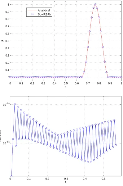
The steep profile of the solution is well captured by the SL-IRBFN scheme as shown in Figure 1. In fact, withN= 61 regularly located points andCF L= 0.5, the numerical solutions are accurate up to 3 digits after the decimal point in the steep region whereas the absolute errors by the scheme can be of order 10−5 in the flat regions. In addition, it can be seen in Figure 1 that there are no
severe errors found right before and after the shock as observed in Lax-Wendroff and second-order Taylor-Galerkin schemes [Donea and Huerta (2003)].
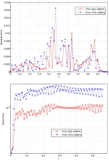
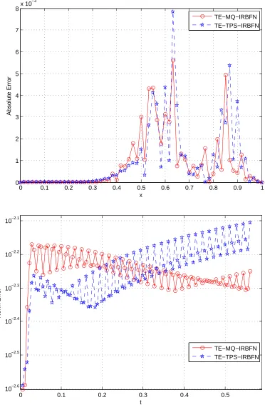
A comparison of accuracy and stability of the TCN-IRBFN scheme using MQ and TPS basis functions is shown in Figure 2. As can be seen from the figure, the MQ-based scheme is more accurate and stable than its counterpart TPS-based scheme. For this test, theβ parameter of MQ-RBF is set to 1.0. Figure 3 shows a comparison of accuracy and stability of the TE-IRBFN schemes using MQ and TPS basis functions. It is observed from this test that TE-IRBFN scheme using MQ-RBF again yields better solution in terms of both accuracy and stability than its TPS-based counterpart.
7.1.1
Test problem 1.2
Consider a convective transport equation
∂u
∂t −(sinx) ∂u
∂x = 0, x∈Ω, t∈(0, π
2], (65)
subject to the initial condition
u(x,0) = sinx (66)
The analytical solution to the problem is
u(x, t) = sin2 tan−1expttanx 2
, (67)
which develops sharp layers near the end points x= 0 and x= 2π. The problem is solved up to time t =π/2 by the Taylor-IRBFN scheme using regularly located points with point spacing as large as 1/10. Figure 4 shows the analytical and numerical solution by the TCN-IRBFN scheme. As can be seen from the figure, sharp layers near the end points are well resolved by the present scheme even with rather large time steps (∆t = 0.1 or CFL=1). In this case, the time-step size depends on the accuracy requirement, not on stability.
For the purpose of investigating the effect of CFL numbers on the accuracy and stability of the new numerical schemes, the test problem is solved by the SL-IRBFN and TE-IRBFN schemes using a set of different CFL numbers. The root mean square errors corresponding to the CFL numbers are calculated as follows.
RM SE=
s Pnt
i=1(un−ue)2
nt , (68)
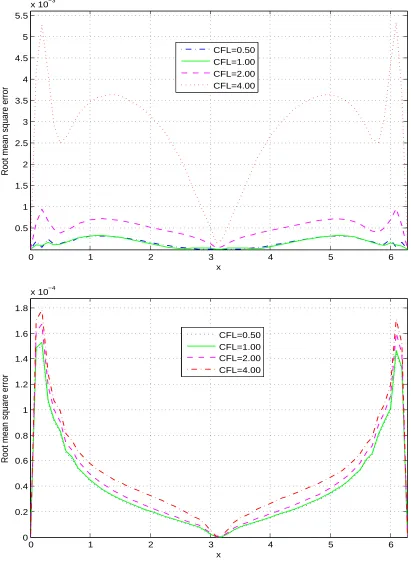
where un and ue are the numerical and exact solutions, respectively; nt is the total number of time steps. As can be seen in Figure 5, for various CFL numbers widely ranging from 0.5 to 4, the root mean square errors are bounded to O(10−3) for the SL-IRBFN scheme, and O(10−4) for
the TE-IRBFN scheme. This verifies the accuracy and stability of the two new numerical schemes. It is observed from the test that on the one hand, the TE-IRBFN scheme is not sensitive to CFL number, meaning that the scheme works fine with high CFL numbers. On the other hand, it is also noted that unlike the SL-IRBFN scheme where the value of the unknown at each time step can be found explicitly, the Taylor-IRBFN scheme requires a solution of a system of equations at each time step.
7.2
Test 2 - Solid body translation
In this test problem, a circle of radius 0.5, initially centered at (-0.75,0), translates to the right due to an external velocity field v = (u, v) = (1,0). The objective of the test is to check the accuracy and stability of the new meshless approach in capturing the moving interface. The circle is translated until time t= 1.0, and the percentage change in the area is calculated for verification purpose.
The problem is solved by the present meshless approach with uniform point spacingdx= 1/15 and time-step size dt= 0.0667. The level set function is advanced in time by the Taylor-IRBFN scheme.
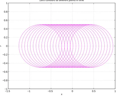
Figure 6 shows zero contours of the level set function at different points in time by the TCN-IRBFN scheme. At each time step of interest, the zero contour of the level set function which is the moving interface is extracted using standard contouring algorithm, and the corresponding area of the circle at those time steps are calculated and compared to the exact area of the original circle. As can be seen from the figure, the circle is well captured by the present approach at different points in time.
Figure 7 shows the percentage change in area at different points in time of interest. It can be seen from the figure that the present approach with the TCN-IRBFN scheme is not only able to accurately capture the moving interface but also stable with the error bounded withinO(10−5) over
the computational time domain. The percentage changes in area at different points in time in this test show that with a coarser point density (dx= 1/15) and a larger time step (dt= 0.0667), the present meshless approach (using either TE-IRBFN or TCN-IRBFN scheme for solving the level set function) gives more accurate solutions (%error ∼ O(10−5)− O(10−3)) than those resulted
from the mesh-based level set scheme (%error ∼ O(10−2)) with denser discretization in space
(dx = 1/80) and time (CF L= 0.9) [Sethian (1999)]. Figure 7 also shows that the TCN-IRBFN scheme yields better result than the TE-IRBFN scheme for this test problem.
It is noted that for such a simple velocity field in this test, the reinitalization step is not needed. In fact, only a mass correction presented in Section§6.4 is performed at each time step in this test. Without the reinitialization step, the present approach is still highly accurate and stable. This verifies the efficiency of the new meshless approach for this basic test problem.
7.3
Test 3 - Rotation of a solid body
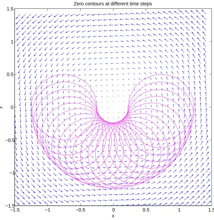
Consider the rotation of a circle of radiusr= 0.5 initially centered at (−0.75,0) in a vortex flow with velocity field (u, v) = (−y, x). It is noted that with such a velocity field, the circle rotates around the coordinate’s origin (0,0) without any deformations. In other words, the circle is considered to be a solid body. An half cycle of rotation is performed by the present meshless approach, and the percentage change in area of the circle during its motion is calculated.
scheme (described in Section§4 in which the IRBFN semi-discrete scheme [Mai-Cao and Tran-Cong (2005)] with the fourth-order Runge-Kutta procedure is used to track particles that arrive at the grid points backward to their departure points over a single time step. The function values at those departure points are then obtained by interpolation with TPS-IRBFN formulation.
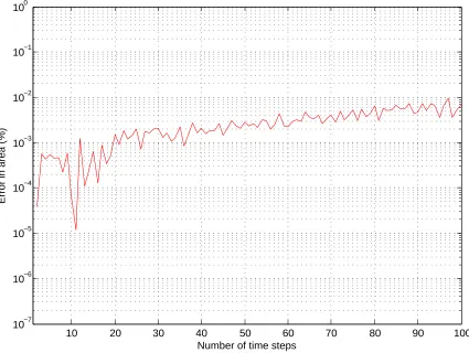
Figure 8 shows the zero contours of the level set function at different points in time. Although using a rather coarse point density and normal time-step size, the present approach still exactly reconstructs the moving circle at the points in time of interest. Figure 9 presents the percentage errors in area at different points in time. With a very coarse point density (dx = 1/12) and a large time-step size (dt= 0.0314), the present meshless approach, using the SL-IRBFN scheme for solving the level set function, gives the solution after an half cycle of rotation with the change/error in area of 0.006970%. In [Sethian (1999)], the same test problem was performed with different grid sizes and the percentage error in area was reported to be 0.09758% with the grid size of 161×161. No conclusion on which (meshless or mesh-based scheme) is better is made for this particular test problem since there is no information about the time-step size used in [Sethian (1999)].
It is noted that the numerical solution for this test is obtained without the reinitialization step. In fact, only a mass correction step is performed at each time step. The numerical result shows that the present approach is accurate and stable with the error bounded within O(10−4)− O(10−3).
It can be concluded that for such a simple velocity field like the one in this test or in Test 2, the reinitialization step is not required provided that a mass correction is performed at each time step. Since no PDEs are solved in the mass correction procedure, saving of computational time is achieved.
7.4
Test 4 - Passive transport of a bubble in a shear flow
In this problem (this example and the following one represent more serious application of the present approach), a bubble with a radius of 0.15, initially centered at (0.5,0.7) moves and deforms in a shear flow with a divergence-free velocity field v= (u, v) defined as follows.
u=−sinπxcosπy, 0≤x, y≤1, t≥0, (69)
v= cosπxsinπy, 0≤x, y ≤1, t≥0. (70)
The problem is solved by the present meshless approach with a point densitydx=dy= 1/50 and time-step sizedt= 0.01. The time-step sizedtis so chosen to satisfy the Courant-Friedreichs-Levy condition [Osher and Fedkiw (2003)].
∆t×max
|u|
dx+
|v|
dy
= CFL, (71)
where the CFL number is chosen to be unity.
In this problem, the level set function is advanced in time by the SL-IRBFN scheme in which the values of the level set function at departure points are obtained via interpolation by the TPS-IRBFN formulation. At the end of each time step, the reinitialization procedure is done by solving equation (20) to steady-state using the semi-implicit IRBFN-based scheme with the fourth-order Runge-Kutta procedure [Mai-Cao and Tran-Cong (2005)]. For the purpose of investigating the effect of the mass correction on the accuracy and stability of the present approach, the reinitialization procedure is done with and without mass correction. The area of the bubble in motion is calculated at each time step and compared to the original area (πR2). The error in area of the bubble in
motion throughout the simulation time is then used to check the stability of the present approach. Figures 10-13 show the zero contours (left) and level set function (right) at different points in time.
Figure 14 shows a comparison of the percentage error in area of the bubble resulted from the present approach with and without mass correction for this problem. As can be seen from the figure, the accuracy of the numerical solution is improved significantly with mass correction. In addition, the percentage error of the bubble is bounded within O(10−5)-O(10−4), indicating the
good stability of the present approach with mass correction.
7.5
Test 5 - Passive transport of four bubbles in a shear flow
The purpose of this example is to demonstrate the ability of the new meshless approach in dealing with topological changes of interfaces in passive transport problems. Four bubbles, each having a
radius of R= 1/6, are initially centered as shown in the top of Figure 15. The bubbles move in a domain of (−1,1)×(−1,1) where there exists a shear flow with the velocity field defined as follows.
u=−ymax
n
1− 1−x2−y24
,0o
8 (x2+y2) (72)
v=xmax
n
1− 1−x2−y24
,0o
8 (x2+y2) (73)
The problem is solved by the present meshless approach with a uniform point spacingdx=dy= 1/60 and time-step size dt = 0.0678. The time-step size dt is so chosen to satisfy the Courant-Friedreichs-Levy condition as in the previous example.
In this example, the level set function is advanced in time by the SL-IRBFN scheme and the reinitialization procedure is done at each time step. For the purpose of investigating the effect of the mass correction on the accuracy and stability of the present approach, the reinitialization procedure is done with and without mass correction. The total area of the bubbles in motion is calculated at each time step and compared to the original value (a0 = 4πR2). The error in area
[image:13.612.141.298.73.146.2]of the bubbles in motion throughout the simulation time is then used to check the stability of the present approach.
Figures 15-17 show the zero contours (left) and level set function (right) at different points in time.
Figure 18 shows a comparison of the percentage error in area of the bubble resulted from the present approach with and without mass correction for this example. As can be seen from the figure, the accuracy of the numerical solution is improved significantly with mass correction. In addition, the percentage error of the bubble is bounded within O(10−5)-O(10−3), indicating the
good stability of the present approach with mass correction.
8
Concluding Remarks
A new meshless approach to capturing moving interfaces in passive transport problems is presented in this paper where the motion and deformation of the moving interfaces are well captured by a unique procedure even with the presence of topological changes. The present approach brings the highly accurate IRBFN method for spatial discretization, the high-order time stepping methods based on semi-Lagrangian or Taylor series expansions and the level set method together for dealing with moving interfaces in an accurate and efficient manner. In this work, a mass correction proce-dure is introduced at each time step to improve the accuracy of the interface reconstruction. The procedure can be used with or without a reinitialization step. Numerical experiments, including some basic tests for the new numerical schemes and the simulation of one or more bubbles moving, stretching and merging in ambient shear flows, show the good capability of the present approach for this particular moving interface problem. textbfacknowledgement: T. Tran-Cong was hosted by the Faculty of Geology and Petroleum Engineering, on his sabbatical at Ho Chi Minh City University of Technology, Ho Chi Minh City, Vietnam. This work is partially supported by the Australian Research Council. These supports are gratefully acknowledged.
References
Allievi, A. and Bermejo, R. (2000). Finite element modified method of characteristics for the Navier-Stokes equations,International Journal for Numerical Methods in Fluids32: 439–464. Atluri, S. (2004). The Meshless Local Petrov-Galerkin (MLPG) Method for Domain & BIE
Dis-cretizations, Tech Science Press, Encino, CA, USA.
Bardi, M. and Osher, S. (1991). The nonconvex multidimensional Riemann problem for Hamilton-Jacobi equations,SIAM Journal on Mathematical Analysis22: 344–351.
Chang, Y., Hou, T., Merriman, B. and Osher, S. (1996). A level set formulation of Eulerian interface capturing method for incompressible fluid flows,Journal of Computational Physics124: 449–464. Crandall, M. and Lions, P. (1984). Two approximations of solutions of Hamilton-Jacobi equations,
Math. Comput.43: 1–19.
Cuvelier, C. and Schulkes, R. (1990). Some numerical methods for the computation of capillary free boundaries governed by the Navier-Stokes equations,SIAM Review32(3): 355–423. Donea, J. (1984). A Taylor-Galerkin method for convective transport problems, International
Journal for Numerical Methods in Engineering20: 101–119.
Donea, J. and Huerta, A. (2003). Finite Element Methods for Flow Problems, John Wiley & Sons Ltd., England.
Floryan, J. and Rasmussen, H. (1989). Numerical methods for viscous flows with moving boundary,
Applied Mechanics Reviews42(12): 323–341.
Hirt, C. and Nichols, B. (1981). Volume of fluid (VOF) method for the dynamics of free boundaries,
Journal of Computational Physics39(1): 201 –225.
Iafrati, A., Mascio, A. and Campana, E. (2001). A level set technique applied to unsteady free surface flows,International Journal for Numerical Methods in Fluids35: 281–297.
Jacqmin, D. (1999). Calculation of two-phase Navier-Stokes flows using phase-field modelling,
Journal of Computational Physics155: 96–127.
Kansa, E. (1990). Multiquadrics - A scattered data approximation scheme with applications to com-putational fluid-dynamics–II. Solutions to parabolic, hyperbolic and elliptic partial differential equations,Computers and Mathematics with Applications 19(8/9): 147–161.
Mai-Cao, L. and Tran-Cong, T. (2005). A meshless IRBFN-based method for transient problems,
CMES:Computer Modeling in Engineering & Sciences18(1): 59–77.
Mai-Duy, N. (2004). Indirect rbfn method with scattered points for numerical solution of pdes,
CMES:Computer Modeling in Engineering & Sciences6: 209–226.
Mai-Duy, N. and Tran-Cong, T. (2001a). Numerical solution of differential equations using multi-quadric radial basis function networks,Neural Networks14: 185–199.
Mai-Duy, N. and Tran-Cong, T. (2001b). Numerical solution of navier-stokes equations using multiquadric radial basis function networks, International Journal for Numerical Methods in
Fluids37: 65–86.
Mai-Duy, N. and Tran-Cong, T. (2003). Approximation of function and its derivatives using radial basis function networks,Applied Mathematical Modelling 27: 197–220.
Mai-Duy, N., Mai-Cao, L. and Tran-Cong, T. (2007). Computation of transient viscous flows using indirect radial basis function networks, CMES:Computer Modeling in Engineering & Sciences 7(2): 149–171.
Moody, J. and Darken, C. (1989). Fast learning in networks of locally-tuned processing units,
Neural Computations1: 281–294.
Oliveira, A. and Baptista, A. (1995). A comparison of integration and interpolation Eulerian-Lagrangian methods,International Journal for Numerical Methods in Fluids21: 183–204. Osher, S. and Fedkiw, R. (2003). Level Set Methods and Dynamic Implicit Surfaces, Vol. 153 of
Applied Mathematical Sciences, Springer, New York.
Osher, S. and Sethian, J. (1988). Fronts propagating with curvature-dependent speed: Algorithms based on Hamilton-Jacobi formulations,Journal of Computational Physics79: 12–49.
Peng, D., Merriman, B., Osher, S., Zhao, H. and Kang, M. (1999). A PDE-based fast local level set method,Journal of Computational Physics155: 410–438.
Sarler, B. (2005). A radial basis function collocation approach in computational fluid dynamics,
CMES:Computer Modeling in Engineering & Sciences7(2): 185–193.
Sethian, J. (1999). Level Set Methods and Fast Marching Methods: Evolving Interfaces in Com-putational Geometry, Fluid Mechanics, Computer Vision, and Materials Science, Cambridge University Press, New York.
Shu, C. and Osher, S. (1989). Efficient implementation of essentially non-oscillatory shock capturing schemes II,Journal of Computational Physics 83: 32–78.
Shu, C., Ding, H. and Yeo, K. (2005). Computation of incompressible navier-stokes equations by local rbf-based differential quadrature method,CMES:Computer Modeling in Engineering &
Sciences7(2): 195–205.
Staniforth, A. and Cote, J. (1991). Semilagrangian integration schemes for atmospheric models -A review,Monthly Weather Review 119: 2206–2223.
Sussman, M. and Fatemi, E. (1999). An efficient, interface-preserving level set redistancing algo-rithm and its application to interfacial incompressible fluid flow., SIAM Journal on Scientific
Computing20(4): 1165–1191.
Sussman, M. and Smereka, P. (1997). Axisymmetric free boundary problems, Journal of Fluid
Mechanics341: 269–294.
Sussman, M., Smereka, P. and Osher, S. (1994). A level set approach for computing solutions to incompressible two-phase flow,Journal of Computational Physics114: 146–159.
Temperton, C. and Staniforth, A. (1987). An efficient two-time level semi-Lagrangian semi-implicit integration scheme,Quart. J. Roy. Meteor. Soc.113: 1025–1039.
Tornberg, A. (2000).Interface Tracking Methods with Application to Multiphase Flows, PhD thesis, Royal Institute of Technology, Stockholm.
Unverdi, S. and Tryggvason, G. (1992). A front-tracking method for viscous, incompressible, multi-fluid flows,Journal of computational physics100: 25–37.
Wang, S., Lim, K., Khoo, B. and Wang, M. (2007). A geometric deformation constrained level set method for structural shape and topology optimization,CMES:Computer Modeling in
0 0.1 0.2 0.3 0.4 0.5 0.6 0.7 0.8 0.9 1 0
0.1 0.2 0.3 0.4 0.5 0.6 0.7 0.8 0.9 1
x
U
Analytical SL−IRBFN
0 0.1 0.2 0.3 0.4 0.5
10−2.5 10−2.4
t
[image:16.612.129.526.65.664.2]Norm Error
Figure 1: Test 1.1: Numerical solution (top) and its
L
∞−
norm error (bottom) by the SL-IRBFN
scheme.
0 0.1 0.2 0.3 0.4 0.5 0.6 0.7 0.8 0.9 1 0
0.002 0.004 0.006 0.008 0.01 0.012 0.014 0.016 0.018
x
Absolute Error
TCN−MQ−IRBFN TCN−TPS−IRBFN
0 0.1 0.2 0.3 0.4 0.5
10−2
t
Norm Error
[image:17.612.134.515.68.628.2]TCN−MQ−IRBFN TCN−TPS−IRBFN
0 0.1 0.2 0.3 0.4 0.5 0.6 0.7 0.8 0.9 1 0
1 2 3 4 5 6 7 8x 10
−3
x
Absolute Error
TE−MQ−IRBFN TE−TPS−IRBFN
0 0.1 0.2 0.3 0.4 0.5
10−2.6 10−2.5 10−2.4 10−2.3 10−2.2 10−2.1
t
Norm Error
[image:18.612.142.514.64.638.2]TE−MQ−IRBFN TE−TPS−IRBFN
Figure 3: Test 1.1: Comparison between the two variants of the TE-IRBFN scheme (using MQ and
TPS basis functions), Absolute error at the last time step (top);
L
∞-norm error with respect to time
(bottom).
0
1
2
3
4
5
6
−1
−0.8
−0.6
−0.4
−0.2
0
0.2
0.4
0.6
0.8
1
x
U
[image:19.612.116.533.60.373.2]Analytical
TCN−IRBFN
0 1 2 3 4 5 6 0.5
1 1.5 2 2.5 3 3.5 4 4.5 5 5.5
x 10−3
x
Root mean square error
CFL=0.50 CFL=1.00 CFL=2.00 CFL=4.00
0 1 2 3 4 5 6
0 0.2 0.4 0.6 0.8 1 1.2 1.4 1.6 1.8
x 10−4
x
Root mean square error
[image:20.612.98.509.71.632.2]CFL=0.50 CFL=1.00 CFL=2.00 CFL=4.00
Figure 5: Test 1.2: Numerical investigation of the accuracy and stability of the present numerical
schemes, root mean square errors corresponding to various values of the CFL number within a rather
wide range (0.5-4) are bounded to
O
(10
−3) for the SL-IRBFN scheme (top), and
O
(10
−4) for the
TE-IRBFN scheme (bottom).
x
y
Zero contours at different points in time
−1.5 −1 −0.5 0 0.5 1
[image:21.612.123.531.184.524.2]−1 −0.8 −0.6 −0.4 −0.2 0 0.2 0.4 0.6 0.8 1
0.2 0.4 0.6 0.8 1 1.2
10−9
10−8
10−7
10−6
10−5
10−4
10−3
10−2
10−1
Time
Error in area (%)
[image:22.612.110.541.173.493.2]TE−IRBFN TCN−IRBFN
Figure 7: Test 2: Percentage errors in area at different points in time. With a coarser point
den-sity (dx
= 1/15) and a larger time step (CF L
= 1.0), the present meshless approach (using
ei-ther TE-IRBFN or TCN-IRBFN scheme for solving the level set function) gives more accurate
so-lutions (%error
∼ O
(10
−5)
− O
(10
−3)) than those resulted from the mesh-based level set scheme
(%error
∼ O
(10
−2)) with denser grid points (81
×
81) and time (CF L
= 0.9) [Sethian (1999)].
The numerical result also shows that the TCN-IRBFN scheme is more accurate and stable than the
TE-IRBFN scheme for this test problem.
x
y
Zero contours at different time steps
−1.5 −1 −0.5 0 0.5 1 1.5
[image:23.612.117.533.146.574.2]−1.5 −1 −0.5 0 0.5 1 1.5
10 20 30 40 50 60 70 80 90 100 10−7
10−6 10−5 10−4 10−3 10−2 10−1 100
Number of time steps
[image:24.612.113.538.200.520.2]Error in area (%)
Figure 9: Test 3: Percentage errors in area at different points in time. With a rather coarse point
density (dx
=
dy
= 1/12) and normal time-step size (dt
= 0.0314), the present meshless approach,
using the SL-IRBFN scheme for advancing the level set function, is quite accurate and stable.
x
y
Initial zero contour
0 0.2 0.4 0.6 0.8 1
0 0.2 0.4 0.6 0.8 1
0 0.5
1
0 0.2 0.4 0.6 0.8 1 −0.5 0 0.5 1
x Initial level set function
y
x
y
Zero contour at t = 0.600
0 0.2 0.4 0.6 0.8 1
0 0.2 0.4 0.6 0.8 1
0
0.5
1
0 0.5 1 −0.2
0 0.2 0.4 0.6 0.8
x Level set function at t = 0.600
[image:25.612.93.514.131.623.2]y
x
y
Zero contour at t = 1.400
0 0.2 0.4 0.6 0.8 1
0 0.2 0.4 0.6 0.8 1
0 0.5
1 0
0.5 1 −0.2
0 0.2 0.4 0.6 0.8
x Level set function at t = 1.400
y
x
y
Zero contour at t = 1.900
0 0.2 0.4 0.6 0.8 1
0 0.2 0.4 0.6 0.8 1
0 0.2 0.4 0.6 0.8 1
0 0.5 1 −0.2
0 0.2 0.4 0.6 0.8
x
Level set function at t = 1.900
[image:26.612.88.513.119.619.2]y
Figure 11: Test 4: The zero contour and the level set function at
t
= 1.40 (top) and
t
= 1.90 (bottom).
x
y
Zero contour at t = 2.400
0 0.2 0.4 0.6 0.8 1
0 0.2 0.4 0.6 0.8 1
0 0.5
1
0 0.2 0.4 0.6 0.8 1 −0.2 0 0.2 0.4 0.6 0.8
x Level set function at t = 2.400
y
x
y
Zero contour at t = 2.900
0 0.2 0.4 0.6 0.8 1
0 0.2 0.4 0.6 0.8 1
0 0.2 0.4 0.6 0.8 1
0 0.5 1 −0.2
0 0.2 0.4 0.6 0.8
x
Level set function at t = 2.900
[image:27.612.88.520.119.623.2]y
x
y
Zero contour at t = 3.400
0 0.2 0.4 0.6 0.8 1
0 0.2 0.4 0.6 0.8 1
0
0.5
1
0 0.5 1 −0.2
0 0.2 0.4 0.6 0.8
x Level set function at t = 3.400
y
x
y
Zero contour at t = 4.000
0 0.2 0.4 0.6 0.8 1
0 0.2 0.4 0.6 0.8 1
0 0.5
1 0
0.5 1 −0.2
0 0.2 0.4 0.6 0.8
x Level set function at t = 4.000
[image:28.612.88.516.112.618.2]y
Figure 13: Test 4: The zero contour and the level set function at
t
= 3.40 (top) and
t
= 4.00 (bottom).
0 50 100 150 200 250 300 350 400 10−7
10−6 10−5 10−4 10−3 10−2 10−1 100 101 102
Number of time steps
Error in area (%)
[image:29.612.114.538.184.516.2]Without mass correction With mass correction
Figure 14: Test 4: Comparison of the percentage error in area of the bubble resulted from the present
approach with and without mass correction. The accuracy of the numerical solution is improved
significantly with mass correction. The error is bounded within
O
(10
−5)-
O
(10
−4x
y
Initial zero contour
−1 −0.5 0 0.5 1
−1 −0.5 0 0.5 1
−1 −0.5
0 0.5 1
−1 0 1 −0.5
0 0.5 1
x Initial level set function
y
x
y
Zero contour at t = 1.357
−1 −0.5 0 0.5 1
−1 −0.5 0 0.5 1
−1 −0.5
0 0.5
1
−1 0
1 0 0.2 0.4 0.6 0.8
x Level set function at t = 1.357
[image:30.612.116.532.115.626.2]y
Figure 15: Test 5: Zero contours and the level set function at t=0 (top) and t=1.357 (bottom).
x
y
Zero contour at t = 3.392
−1 −0.5 0 0.5 1
−1 −0.5 0 0.5 1
−1 −0.5 0
0.5 1
−1 −0.5
0 0.5
1 0 0.2 0.4 0.6 0.8
x
Level set function at t = 3.392
y
x
y
Zero contour at t = 6.105
−1 −0.5 0 0.5 1
−1 −0.5 0 0.5 1
−1 −0.5
0 0.5
1
−1 0 1
0 0.2 0.4 0.6 0.8
x Level set function at t = 6.105
[image:31.612.89.514.91.632.2]y
x
y
Zero contour at t = 8.141
−1 −0.5 0 0.5 1
−1 −0.5 0 0.5 1
−1 −0.5
0 0.5
1
−1 0 1
0 0.2 0.4 0.6 0.8
x Level set function at t = 8.141
y
x
y
Zero contour at t = 10.176
−1 −0.5 0 0.5 1
−1 −0.5 0 0.5 1
−1 −0.5
0 0.5
1
−1 0 1
0 0.2 0.4 0.6 0.8
x Level set function at t = 10.176
[image:32.612.98.511.105.634.2]y
Figure 17: Test 5: Zero contours and the level set function at t=8.141 (top) and t=10.176 (bottom).
20 40 60 80 100 120 140 160 180 200 10−6
10−5 10−4 10−3 10−2 10−1 100 101
Number of time steps
Error in area (%)
[image:33.612.115.541.184.511.2]Without mass correction With mass correction
Figure 18: Test 5: Comparison of the percentage error in area of the bubbles resulted from the present
approach with and without mass correction. The accuracy of the numerical solution is improved
significantly for the latter case. The error in total area of the bubbles in motion is bounded within
O
(10
−5)-
O
(10
−3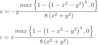

![Figure 7: Test 2: Percentage errors in area at different points in time. With a coarser point den-sity (ther TE-IRBFN or TCN-IRBFN scheme for solving the level set function) gives more accurate so-lutions (%The numerical result also shows that the TCN-IRBFN scheme is more accurate and stable than thedx = 1/15) and a larger time step (CFL = 1.0), the present meshless approach (using ei-error ∼ O(10−5) − O(10−3)) than those resulted from the mesh-based level set scheme(%error ∼ O(10−2)) with denser grid points (81 × 81) and time (CFL = 0.9) [Sethian (1999)].TE-IRBFN scheme for this test problem.](https://thumb-us.123doks.com/thumbv2/123dok_us/250359.58851/22.612.110.541.173.493/percentage-dierent-accurate-numerical-accurate-meshless-approach-resulted.webp)