Bayesian Hidden Topic Markov Models

(1)

Rochester Institute of Technology

RIT Scholar Works

Theses Thesis/Dissertation Collections

5-11-2017

Bayesian Hidden Topic Markov Models

Kenneth Tyler Wilcox

[email protected]

Follow this and additional works at:http://scholarworks.rit.edu/theses

This Thesis is brought to you for free and open access by the Thesis/Dissertation Collections at RIT Scholar Works. It has been accepted for inclusion in Theses by an authorized administrator of RIT Scholar Works. For more information, please [email protected].

Recommended Citation

(2)

by

A thesis submitted in partial fulfillment of the requirements for the degree of

Master of Science

in

Applied Statistics

in the

School of Mathematical Sciences

of the

College of Science

of the

Rochester Institute of Technology

Committee in charge:

Associate Professor Ernest Fokou´e, Chair Assistant Professor Cecilia Alm Assistant Professor Emily Prud’hommeaux

Assistant Professor Wei Qian Professor Joseph Voelkel

(3)

by

(4)

1

Abstract

by

Master of Science in Applied Statistics

Rochester Institute of Technology

Associate Professor Ernest Fokou´e, Chair

Recent developments in topic modeling for text corpora have incorporated Markov models

in the latent space to better learn contextual content. Known as the Hidden Topic Markov

Model (HTMM), this natural extension of probabilistic mixture models relaxes the

“bag-of-words” assumption of the foundational latent Dirichlet allocation topic model by allowing

the discrete latent variables, or topics, to follow a special first-order Markov process.

Pa-rameter estimation is performed using an expectation-maximization (EM) algorithm with

fixed dimensionality of the topic space (Gruber, Rosen-Zvi, and Weiss 2007). I fully derive

the state space and EM algorithm for the HTMM. I then extend the Hidden Topic Markov

Model (HTMM) into a fully Bayesian framework using a Gibbs sampler. The necessary full

conditional distributions are derived and a Gibbs sampling algorithm proposed. I implement

both the HTMM EM algorithm (Gruber, Rosen-Zvi, and Weiss 2007) and the HTMM Gibbs

sampling algorithm in the R and C++ programming languages. The performance of both

inferential algorithms is evaluated on twelve simulated data sets and on a collection of

pro-ceedings from the Conference on Neural Information Processing Systems (NIPS). The results

suggest that the Gibbs sampling algorithm provides better recovery of the topic space than

(5)

2

point estimates with both algorithms. The convergence of the Gibbs sampler is studied and

is reliable for reasonably large data sets. Evaluation of both algorithms on the NIPS corpus

suggests that the HTMM is better able to handle polysemy than LDA and provides coherent

and contiguous topics. Predictive accuracy measured by perplexity is better on training

and test documents using the HTMM than using LDA on the NIPS corpus. Introducing

Markovian dynamics in topical space provides better topical segmentation of a corpus and

increased predictive accuracy for unseen documents.

Gibbs sampler; hidden Markov models; hierarchical Bayes; latent variable modeling; mixture

(6)

i

To Jess

(7)

ii

List of Figures

2.1 Graphical model of probabilistic Latent Semantic Indexing . . . 8

2.2 Graphical model of Latent Dirichlet Allocation . . . 10

2.3 Graphical model of mixture of unigrams . . . 11

2.4 Graphical model of the correlated topic model . . . 14

2.5 (a) Graphical model of the latent Dirichlet allocation topic model. (b) Graphical model of the hidden topic Markov model. Word generation is drawn explicitly to highlight the topic independence in LDA versus the topic Markov chain in HTMM. 17 3.1 Metropolis-Hastings sampler . . . 22

3.2 Gibbs sampler . . . 24

3.3 Gibbs sampler for univariate latent variable model . . . 26

3.4 Empirical posterior distribution of theta . . . 27

3.5 Graphical model of a mixture of two Gaussians . . . 29

3.6 Gibbs sampler for mixture of two Gaussians . . . 32

3.7 Empirical posterior distributions for a mixture of two Gaussians. . . 33

4.1 Forward algorithm . . . 38

4.2 Backward algorithm . . . 39

4.3 Compute update probabilities . . . 44

4.4 Expectation-Maximization algorithm for discrete hidden Markov model . . . 46

5.1 Forward algorithm for Hidden Topic Markov Model . . . 55

5.2 Backward algorithm for Hidden Topic Markov Model . . . 57

6.1 Gibbs sampler for the Hidden Topic Markov Model . . . 76

7.1 Convergence of log-likelihood for HTMM-EM algorithm (left). Convergence of estimated transition probability (right). . . 83

7.2 Sample path of transition probability from simulated data set 1. . . 84

7.3 Posterior distribution of transition probability from simulated data set 1. . . 85

7.4 Sample path of topic proportions in the first document of simulated data set 1. . 86

(10)

v

7.6 Sample path of topic-word probabilities for the first word from simulated data

set 1. . . 88

7.7 Posterior distributions of topic-word probabilities for the first word from simu-lated data set 1. . . 89

7.8 Sample path of transition probability from simulated data set 7. . . 90

7.9 Posterior distribution of transition probability from simulated data set 1. . . 91

7.10 Sample path of topic proportions in the first document of simulated data set 7. . 92

7.11 Posterior distribution of topic proportions in the first document from simulated data set 7. . . 92

7.12 Sample path of topic-word probabilities for the first word from simulated data set 7. . . 93

7.13 Posterior distributions of topic-word probabilities for the first word from simu-lated data set 7. . . 94

7.14 Convergence of log-likelihood for HTMM-EM algorithm (left). Convergence of estimated epsilon parameter (right) . . . 95

7.15 The ten most probable words for topics 13, 16, 55, and 75 from the NIPS LDA model . . . 96

7.16 Sample topics from NIPS HTMM model . . . 98

7.17 Sample topic proportions from NIPS LDA model . . . 99

(11)

vi

List of Tables

7.1 Attributes of data sets simulated from the generative HTMM . . . 78

7.2 Performance of HTMM-EM on simulated data . . . 79

(12)

vii

Acknowledgments

I would like to thank my advisor Dr. Ernest Fokou´e for his unfailing support and inspiration.

If it were not for your encouragement, I would not have completed this work and would not

be embarking on a PhD. I would like to thank my committee for their wisdom and support.

I would like to thank my parents for never doubting me and encouraging me to persevere.

(13)

1

Chapter 1

Introduction

1.1

Problem Statement

The Hidden Topic Markov Model of Gruber, Rosen-Zvi, and Weiss (2007) is extended into

a Bayesian framework: posterior distributions are derived and a Gibbs sampling algorithm

is developed and implemented in the R and C++ programming languages. The

expectation-maximization algorithm for the Hidden Topic Markov Model is derived fully along with a

special extension of the forward-backward and Viterbi algorithms for hidden Markov models

in order to perform inference. The performance of the expectation-maximization algorithm

for the Hidden Topic Markov Model proposed by Gruber, Rosen-Zvi, and Weiss and the novel

Gibbs sampling algorithm is evaluated in a simulation study and on a real-world corpus of

conference proceedings.

1.2

Overview

The accessibility of vast quantities of text-based information has spurred the development of

many computational and statistical approaches to extract and summarize text-based data.

(14)

CHAPTER 1. INTRODUCTION 2

set of natural language processing problems. Primary tasks when modeling discrete data like

text often include classifying documents or queries, summarizing a body of text, information

retrieval, novelty detection, authorship identification, and structural analysis. This thesis

concerns itself with topic modeling; topic models offer a statistical model of textual structure.

In this thesis, a novel extension of recent efforts to learn topical representations that are

more semantically coherent through the use of hidden Markov models is proposed using a

fully Bayesian framework. This is a marked departure from Blei, Ng, and Jordan (2003),

whose seminal latent Dirichlet allocation (LDA) assumes that topics are independently

dis-tributed in a document. While LDA has become popular for topic modeling, its underlying

assumptions ignore the meaning created by the order of words in sentences, paragraphs,

and documents. The introduction of a Markov process over the topics is expected to better

model the sequential meaning contained in sentences and paragraphs by assuming that the

topic of a sentence depends on the topic of the previous sentence. However, introducing a

Markov process into the latent space makes estimation and inference non-trivial in this

con-text. Analytical solutions can be intractable, necessitating computational solutions such as

the expectation-maximization (EM) algorithm or sampling algorithms like the Gibbs

sam-pler. The inferential approach for the Hidden Topic Markov Model proposed by Gruber,

Rosen-Zvi, and Weiss (2007) relies on an EM algorithm (Dempster, Laird, and Rubin 1977).

It is well known that the EM algorithm is not guaranteed to converge to a global maximum,

which motivates the use of a Gibbs sampling approach since Gibbs sampling produces a

Markov chain that will converge to the true posterior distribution in the limit (Gelfand and

Smith 1990), although Gibbs samplers may not converge in practice when taking a finite

sample. Another advantage of Gibbs sampling is the ability to recover the posterior

distri-bution of model parameters. The EM algorithm treats model parameters as fixed values,

and yields point estimates of parameters rather than distributions.

The Hidden Markov Topic Model of Andrews and Vigliocco (2010) proposes a Gibbs

sampler for a similar model that makes use of a traditional hidden Markov model, but relies

(15)

CHAPTER 1. INTRODUCTION 3

other time-dependent topic processes have been introduced by others (Blei and Moreno 2001;

Blei and Lafferty 2006; Wang and McCallum 2006), there does not appear to be any Bayesian

extensions of the Hidden Topic Markov Model.

The Hidden Topic Markov Model aims to produce more coherent topics than LDA by

capturing semantic relationships within and between sentences through its use of Markovian

dynamics in the topic space that LDA is unable to identify. Another potential benefit of

the Markov process is the extraction of topics that are more robust to chaining than LDA.

Chained topics occur when two or more distinct subsets of words are combined with words

that are ambiguous since they can belong to more than one subset (Boyd-Graber, Mimno,

and Newman 2014). Allowing a first-order Markov process to drive the topic transitions is

expected to reduce the negative impact of polysemy – multiple meanings for a single word –

on topic quality. A fully Bayesian framework for such a topic model allows the approximation

of the posterior distributions.

1.3

Organization

The contents of this proposal are organized into four sections. Chapter 1 motivates and

introduces the work presented in this thesis. In Chapter 2, related work in the context of

document analysis and topic modeling is reviewed with the objective of 1) arguing that a

hierarchical probabilistic model can represent the statistical structure of documents and 2)

motivating the departure from the “bag-of-words” assumption common to many topic models

as a means of obtaining more coherent topic assignments. In Chapter 3, the Gibbs sampler

and its use in Bayesian approaches to statistical modeling is discussed and the use of Gibbs

sampling for continuous latent variable models and discrete latent variable mixture modeling

is illustrated. Chapter 4 presents the hidden Markov model to motivate its use in topic

modeling. Chapter 5 introduces the state space required by the Hidden Topic Markov Model

and presents derivations of a special forward-backward algorithm, expectation-maximization

(16)

CHAPTER 1. INTRODUCTION 4

of the Hidden Topic Markov model, derives full conditional distributions for the model

parameters and state space, and proposes a Gibbs sampling algorithm. Chapter 7 studies

the performance of the EM and Gibbs sampling algorithms on simulated data and then

compares the Hidden Topic Markov Model to Latent Dirichlet Allocation on a real-world

(17)

5

Chapter 2

Related Work

2.1

Document Analytics and Information Retrieval

Early foundational efforts in information retrieval relied primarily on vector representations

of documents using simple word frequencies in a document or transformations of those

fre-quencies such as tf-idf (Salton and McGill 1983). In tf-idf, term or word frequencies in each

document are counted (tf) and then weighted by the inverse of the number of documents

in the corpus (idf) to obtain the tf-idf measure. Frequently, term frequencies and inverse

document frequencies are both normalized to avoid overemphasizing overly common terms

or unusually rare terms. By representing a document as a vector of term frequencies, some

amount of compression is achieved since the original text no longer needs to be retained.

Comparisons of word frequencies and patterns can be performed directly on the vectorized

representations. Indeed, one can consider suitably normalized term frequencies and

docu-ment frequencies as empirical probability distributions of terms over a docudocu-ment or corpus.

A corpus can be represented in matrix form as a term-document matrix where a corpus’s

vocabulary of terms are represented as rows and the documents in the corpus are represented

as columns. One major drawback of this approach, however, is that minimal reduction is

(18)

CHAPTER 2. RELATED WORK 6

tasks such as information retrieval (Blei, Ng, and Jordan 2003; Salton and McGill 1983).

2.2

Latent Semantic Indexing

Latent semantic indexing (LSI) was an initial effort to improve document retrieval for

query-based searches. Deerwester et al. (1990) noted that document retrieval solely query-based on term

matching is unreliable for two primary reasons. First, query terms may not be contained

in the document or its metadata; a relevant document without exact term matches will not

be returned. This problem is known as synonymy. Second, polysemy – multiple meanings

for a given word – can lead to the retrieval of irrelevant documents; these documents will

contain matches to a query term, but the documents’ terms may have entirely different

meanings than the query’s intent. Methods relying solely on the original term-document

matrix are prone to suffering from both synonymy and polysemy; while exact matches of a

query term may not exist in the corpus, synonymous words might. Similarly, polysemous

words can inappropriately match query terms as exact matches when the meaning of the

word in a document does not match the meaning in the query. Again, using the original

document-term matrix, it is impossible to disambiguate multiple word senses. Projection of

the document-term matrix into a lower-dimensional space can encode relationships among

synonymous words and disambiguate word senses for polysemous words by embedding related

words and multiple word senses in a subspace that captures relationships like synonymy and

polysemy.

Seminal work by Deerwester et al. (1990) suggested searching for a latent space where

projections of the term-document matrix into the latent space yielded a lower-dimensional

representation. Furthermore, they proposed that such a projection should capture any

as-sumed underlying semantic structure in the original term-document matrix. Their approach

used singular-value decomposition on the term-document matrix to reduce the

dimension-ality from V to K such that K < V where V is the size of the vocabulary of a corpus and

(19)

doc-CHAPTER 2. RELATED WORK 7

uments and terms are obtained by this matrix factorization. The complexity of the latent

representation is controlled by K. The LSI approximation of the original term-document

matrix can be shown to minimize the Frobenius norm and as such yields a rank-K optimal

approximation of the original document-term matrix (Hofmann 1999).

Queries can be projected into the resulting latent space and document similarity is

as-sessed by comparing the latent projection of the query to the latent representation of

neigh-boring documents using vector-based similarity measures such as the inner product. Methods

like factor analysis or clustering operate on document similarity matrices or term similarity

matrices and are unable to capture relationships between terms and documents.

Unfortunately, LSI assumes strictly linear relationships between terms and documents

and provides no probabilistic generative model of a corpus. Subsequent developments such

as probabilistic LSA and latent Dirichlet allocation (LDA) provide such a framework.

2.3

Probabilistic Latent Semantic Indexing

A critical development in latent representation of discrete data extended latent semantic

indexing (Deerwester et al. 1990)[LSI] by assuming a generative model of terms and topics

for each document in a corpus. Rather than find a latent representation of a corpus using a

geometric orthogonal norm as in LSI, probabilistic LSI (pLSI) fit a latent projection of the

term-document matrix by maximum likelihood for the generative model (Hofmann 1999).

From an application perspective, LSI is compelling since the singular value decomposition of

the term-document matrix can scale well for large data sets. However, the use of generative

probabilistic models for corpora tends to outperform the simplistic LSI model, though they

may not scale as easily (Hofmann 1999).

Probabilistic LSI assumes a common generative model (shown in Figure 2.1) for each

document in which a documentd is chosen according to p(d). A latent variable or topicz is

then chosen according top(z|d). Formally, a topic is a distribution over the vocabulary of all

(20)

CHAPTER 2. RELATED WORK 8

the “bag-of-words” assumption, documents are assumed to be independent and words w in

a document are assumed to be drawn independently given topic z. Hofmann proposed an

expectation-maximization solution. Documents can then be described by document-specific

distributions of topicsp(z|d) instead of distributions of the entire vocabulary.

Nd M d

[image:20.612.218.392.207.296.2]

z w

Figure 2.1: Graphical model of probabilistic Latent Semantic Indexing

The distribution of the V-dimensional vocabulary is multinomially distributed over M

documents in the pLSI framework. Using the latent space representation, the words are

multinomially distributed as a sub-simplex over K < M topics. Therefore, information

retrieval can be performed by identifying words in the document space where p(w|d) gives

the location of words w on documents d, d ∈ {1, . . . , D}. Alternatively, a more efficient

representation identifies words in the topic space where p(w|z) gives the location of words

w on topics z, z ∈ {1, . . . , K}. Just as the latent vectors in LSI can be used for similarity

comparisons in information retrieval, p(w|z) can be used equivalently.

2.4

Latent Dirichlet Allocation

While pLSI represents documents as a set of the mixing proportions for the topics (i.e.,

a probability distribution on the fixed topics), it does not model the documents from a

probabilistic model. As a result, there are K(M +V) parameters to learn for K topics,

M documents, and a vocabulary of V words. As a result, the number of parameters grows

(21)

CHAPTER 2. RELATED WORK 9

outside the training set (Blei, Ng, and Jordan 2003), prohibiting generalization of the pLSI

model outside the training corpus.

Latent Dirichlet allocation (LDA) resolves these limitations by providing a probabilistic

generative model of the documents, resulting in K+KV parameters to learn and further

allowing for unseen documents to be classified. The “bag-of-words” assumption in pLSI is

preserved in LDA such that the words are assumed to be independent given topics and the

topics are independent conditioned on the Dirichlet random variableθdfor a given document.

The generative model for LDA is similar to that of pLSI, except that LDA assumes a

probabilistic model of the documents in addition to that of the topics and words. Latent

Dirichlet Allocation assumes that the corpus contains M documents where each document

d∈ {1, . . . , M} is generated by the following process:

1. Draw the number of words in the document Nd∼Poisson(ψ)

2. Draw θd∼Dirichlet(α)

3. For each word wn in document d, n∈ {1, . . . , Nd}

a) Draw topiczn∼Multinomial(θd)

b) Draw word wn|zn ∼Multinomial(βzn)

The topic distribution depends on the K-dimensional random variableθdwhich is drawn

once for each document. The words are drawn independently from a multinomial

parame-terized by β whereβ is aK×V matrix of the conditional probabilities of wordj given topic

i, p(wj|zi = 1). Parameters α and β are corpus-level parameters that are the same for all

documents while θ is a document-level parameter. Note that symmetric prior distributions

are used forθd where the parameters for the Dirichlet prior are all equal toα. The graphical

model for the original LDA model (Blei, Ng, and Jordan 2003) is shown in Figure 2.2.

As a result of the structure of the generative model, all documents share a common set of

(22)

CHAPTER 2. RELATED WORK 10

K

Nd M η

β

α

θ z w

Figure 2.2: Graphical model of Latent Dirichlet Allocation

distribution of the topic mixtureθd, theNd topicsz1, . . . , zNd, andNdwords w1, . . . , wNd can

be written as

p(θd, z1, . . . , zNd, w1, . . . , wNd|α, β) =p(θd|α)p(z1, . . . , zNd|θd)p(w1, . . . , wNd|z1, . . . , zNd, β).

(2.1)

Taking advantage of the conditional independence of the Ndtopics givenθd, equation 2.1

can be rewritten as

p(θd, z1, . . . , zNd, w1, . . . , wNd|α, β) =p(θd|α) Nd

Y

n=1

p(zn|θd)p(wn|zn, β). (2.2)

By marginalizing out the document Dirichlet parameter θd and the topics in equation

2.2, the marginal distribution of a document is

p(w1, . . . , wNd|α, β) =

Z

θd

p(θd|α) Nd

Y

n=1 X

zn

p(zn|θd)p(wn|zn, β)

!

dθd. (2.3)

Furthermore, the probability of a corpus D can be obtained simply since the documents

(23)

CHAPTER 2. RELATED WORK 11

p(D|α, β) = p(w1,w2, . . . ,wM|α, β)

= M

Y

d=1

p(wd|α, β)

= M

Y

d=1 Z

θd

p(θd|α) Nd

Y

n=1 X

zn

p(zn|θd)p(wn|zn, β)

!

dθd. (2.4)

Finally, the joint distribution of words and topics for a document can be obtained by

marginalizing outθd:

p(w1, . . . , wNd, z1, . . . , zNd|α, β) =

Z

p(θd|α) Nd

Y

n=1

p(zn|θd)p(wn|zn)

!

dθd. (2.5)

One simpler alternative to LDA, a mixture of unigrams (Nigam et al. 2000), represents

documents as word distributions conditioned on a single topic (shown in Figure 2.3):

p(w1, . . . , wNd) =

X

z p(z)

Nd

Y

n=1

p(wn|z). (2.6)

Nd M

[image:23.612.215.400.412.557.2]

z w

Figure 2.3: Graphical model of mixture of unigrams

This much simpler mixture model has been shown to inadequately represent large corpora

(Blei, Ng, and Jordan 2003). However, it is informative to view LDA in the context of a

mixture of unigrams since LDA can be considered as a continuous mixture of unigrams if the

(24)

CHAPTER 2. RELATED WORK 12

p(w1, . . . , wNd|θd, β) =

X

zd

p(w1, . . . , wNd|z1, . . . , zNd, β)p(z1, . . . , zNd|θd). (2.7)

This results in a representation of documents from LDA as a continuous mixture:

p(w1, . . . , wNd|α, β) =

Z

p(θd|α) Nd

Y

n=1

p(wn|θd, β)

!

dθd. (2.8)

Here, (wn|θd, β) is a random variable and p(θd|α) defines mixture weights. Most

interest-ingly, the LDA continuous mixture of unigrams only requires K parameters to estimate for

p(θd|α) instead of the K−1 parameters needed for p(z) in the simple mixture of unigrams

model shown in Figure 2.3 while improving the quality of topic allocation substantially.

Blei, Ng, and Jordan (2003) used a variational Bayes algorithm to estimate the

param-eters and topics of the LDA model and demonstrated marked improvement over simple

unigrams, mixtures of unigrams, and pLSI, establishing LDA as a standard for topic

model-ing. However, a fully Bayesian solution was developed using Gibbs sampling (Griffiths and

Steyvers 2002, 2004). More recently, a faster collapsed Gibbs sampler for LDA was proposed

by Porteous et al. (2008).

2.5

Departures from the “Bag-of-Words” Assumption

The popularity and success of LDA (Blei, Ng, and Jordan 2003) spurred an active body

of research to extend LDA beyond its limiting assumptions. As mentioned in section 2.4,

the hierarchical Bayesian model proposed for LDA assumes (unrealistically) that the words

are exchangeable given a topic and that the documents are exchangeable within a corpus.

When treating a topic as a collection of related words, it is reasonable to ignore the meaning

created in natural language by the order of words in a sentence, the order of sentences

in a paragraph, the order of paragraphs in a document, and even the order of documents

in a corpus. Treating a corpus as an unordered collection of documents is reasonable in

(25)

CHAPTER 2. RELATED WORK 13

literature on document analysis over the 20th century. While the “bag-of-words” assumption

is computationally convenient, improvements to topic modeling have generally been driven

by efforts to relax the assumption of independent topics or the assumption of independent

documents.

Correlated Topic Modeling

One approach to inducing a covariance structure in the LDA framework takes advantage of

the hierarchical structure of the model. Blei and Lafferty (2005) introduced correlated topic

models (CTM) to capture the covariance structure of topics. This allows for correlations

as well as independence among topics. The crucial difference between LDA and CTM is

the use of a logistic-normal distribution to model topic proportions instead of a Dirichlet

distribution.

Much like LDA, the correlated topic model assumes that the corpus contains M

docu-ments where each document d∈ {1, . . . , M} is generated by the following process:

1. Draw the number of words in the document Nd∼Poisson(ψ)

2. Draw ηd∼N(µ,Σ)

3. For each word wn in document d

a) Draw topiczn|ηd∼Multinomial(f(ηd))

b) Draw word wn|zn ∼Multinomial(βzn)

where f(ηd) = Pexpηi

jexpηj. The CTM graphical model is shown in Figure 2.4

Blei and Lafferty (2005, 2007) proposed a variational algorithm to perform inference for

CTM. Their results suggested that CTM provides a better fit to corpora than LDA and is

better able to represent larger numbers of topics. Recent work has examined correlated topic

modeling using a probit-normal model instead of the logistic-normal model of CTM (Yu and

(26)

CHAPTER 2. RELATED WORK 14

Nd M

β

µ

Σ η z w

Figure 2.4: Graphical model of the correlated topic model

Dynamic Topic Modeling

While correlated topic modeling (CTM) allows for inference on the topic correlation

struc-ture to be performed, it does not allow for the evolution of topics over time. Blei and Lafferty

(2006) proposed an alternative extension of LDA that, like the correlated topic model,

re-laxes the independence assumption for topics. Rather than model the correlation structure

of topics, they assume that documents develop in a Gaussian time series and that topics in a

given interval of the document time span follow another Gaussian time series. Topic

propor-tions are assumed to follow a Dirichlet distribution as in LDA (Blei, Ng, and Jordan 2003)

and CTM (Blei and Lafferty 2005). Inference is performed using variational approximation

of the posterior distributions. Blei and Lafferty (2006) demonstrated that the dynamic topic

model outperformed static LDA topic models. The development of the dynamic topic model

was preceded by a simpler hidden Markov model approach to topic identification by Blei

and Moreno (2001) that solely focused on unstructured streams of words.

Other attempts to relax the “bag-of-words” assumption have been proposed. Wang and

McCallum (2006) developed a modified version of LDA that allows topics to develop over

time. They place a beta distribution over a normalized continuous time index and learn the

distribution of topics and time by Gibbs sampling. Wallach (2006) developed a hierarchical

(27)

CHAPTER 2. RELATED WORK 15

Dirichlet language model (MacKay and Peto 1995). In this model, the probability of a word

widepends on the previous wordwi−1as well as the topicsz. This effectively extends LDA by

imposing a first-order Markov process on the words in a document and relies on a Gibbs EM

algorithm to perform inference. Performance was better using this hybrid model than both

LDA and the hierarchical Dirichlet language model. A similar model was proposed within the

cognitive science community by Griffiths, Steyvers, and Tenenbaum (2007). Other notable

approaches to topic modeling include syntactic topic models (Boyd-Graber and Blei 2009),

constrained topic assignments (Chen et al. 2009), network analysis (Zhang, Zhu, and Zhang

2013; Bouveyron, Latouche, and Zreik 2016), author-topic models (Rosen-Zvi et al. 2010),

P’olya urn topic models (Mimno et al. 2011), spectral LDA (Anandkumar et al. 2012), neural

network topic models (Wan, Zhu, and Fergus 2012), hidden stochastic automata (Andrews

2013), and augmented max-margin topic models (Zhu et al. 2014). For an accessible review

of the development of topic modeling, see Blei (2012).

2.6

Hidden Topic Markov Modeling

Improved topic quality and predictive performance relative to latent Dirichlet allocation

(LDA) have been achieved by using Markov modeling for the observed words (Wallach 2006,

bigrams). Gruber, Rosen-Zvi, and Weiss (2007) noted that it would be reasonable to adopt

a Markov process in the latent space since it is reasonable to assume that topics would

change over time in a given document. Therefore, they modified LDA by introducing a

hidden Markov model (HMM); this is similar to the work of Blei and Moreno (2001), though

that model does not allow for a mixture of topics in a document or segment of text. The

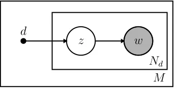
hidden topic Markov model (HTMM) of Gruber, Rosen-Zvi, and Weiss (2007) assumes that

topics are likely to be contiguous throughout a document; this property is modeled with a

first-order discrete Markov chain in the topic space. Specifically, the HTMM assumes that

topics are fixed for a sentence so that all words in a sentence share a single topic. In the

(28)

CHAPTER 2. RELATED WORK 16

can be composed of multiple topics. In the HTMM, topics in a document are dependent on

θd and transition indicator variables ψn, n ∈ {1, . . . , Nd}, where ψ ∈ {0,1}. When ψn = 1,

a new topic zn is drawn according to θd and when ψn = 0, the topic is not changed so

zn = zn−1. Since sentences are assumed to contain a single topic, the Markov chain is only

allowed to change state at the first word of each sentence (i.e., ψn = 0 for words other than

the first words in a sentence). The generative model of a document as shown in Figure 2.5

is described below:

1. For z ∈ {1, . . . , K}

Draw βz ∼Dirichlet(η)

2. Drawθd∼Dirichlet(α)

3. Set ψ1 = 1

4. For each word wn in documentd

a) If wn begins a sentence

Draw ψn∼Binomial()

Else ψn = 0

b) For n∈ {1, . . . , ND}

i. If ψn== 0

zn:=zn−1

Elsezn ∼Multinomial(θd)

ii. Draw word wn|zn ∼Multinomial(βzn)

One disadvantage of the hidden topic Markov model (HTMM) is its storage requirements.

While latent Dirichlet allocation (LDA) and other “bag-of-words” topic models use a

term-document matrix as input, HTMM requires the entirety of each term-document. The cost of

storing the entire corpus is balanced by allowing for more expressive representations of

documents. Perhaps most notably, words are more likely to be drawn from multiple topics

(29)

CHAPTER 2. RELATED WORK 17

Nd _M

... ...

(a)

η β α

θ

z1

z2

zNd

w1

w2

wNd

Nd _M

... ...

(b)

η β α

θ

ψ2

ψNd

z1

z2

zNd

w1

w2

wNd

Figure 2.5: (a) Graphical model of the latent Dirichlet allocation topic model. (b) Graphical model of the hidden topic Markov model. Word generation is drawn explicitly to highlight the topic independence in LDA versus the topic Markov chain in HTMM.

for better disambiguation of polysemous words. LDA tends to assign a given word to a single

or very few topics regardless of where the word occurs in a document or in a corpus. This is

undesirable, for example, if a mathematical paper discussing support vector machines also

referred to the support of a grant in its acknowledgments. Gruber, Rosen-Zvi, and Weiss

(2007) showed that for this example, HTMM is capable of assigning the word support in

the support vector machine context to a mathematical topic and the word support in the

acknowledgements section to a document metadata section. The HTMM may be of particular

interest for natural language processing due to its ability to better capture and disambiguate

these different word senses.

Gruber, Rosen-Zvi, and Weiss (2007) make use of the well-studied Hidden Markov Model

(HMM) to approximate the posterior probabilities. Conditioned onβandθ, the hidden topic

Markov model is a form of HMM so the forward-backward algorithm and the EM algorithm

can be easily used for parameter estimation. In this framework, latent variables zn and

driving variables ψn are drawn from p(zn, ψn|d, w1, . . . , wNd;θd, β, ) where θd, β, and are

considered parameters to be estimated. The joint conditional distribution of zn and ψn is

computed with the forward-backward algorithm for HMM and θd, β, are updated in the

(30)

CHAPTER 2. RELATED WORK 18

While the authors acknowledged that the EM algorithm may be less preferable than a

Gibbs sampler since EM is known to converge to local optima instead of a global optimum,

they argued that their EM algorithm was robust to various initializations. In this thesis,

I derive a Gibbs sampler to provide a Bayesian alternative to the EM algorithm.

Further-more, I am interested in studying the structure of the resulting topic model which is better

accomplished by approximating the joint posterior distribution of the model parameters by

Gibbs sampling than by point estimates alone. Results from Gruber, Rosen-Zvi, and Weiss

(2007) suggested that the HTMM provided lower perplexity scores than LDA which

indi-cated that HTMM better predicted the words in a new corpus. Furthermore, qualitative

analysis suggested that polysemy or word senses were better disambiguated using HTMM

than LDA. Unfortunately, perhaps due to lack of space for publication, Gruber, Rosen-Zvi,

and Weiss (2007) did not provide the derivation of the EM algorithm used for the HTMM.

I derive their EM algorithm, a special forward-backward algorithm, and a special Viterbi

algorithm and then derive a Gibbs sampling algorithm for inference and estimation. Finally,

the performance of the HTMM are assessed in a simulation study and on a real-world corpus.

It is worth noting that the Hidden Markov Topic Model proposed by Andrews and

Vigliocco (2010) is similar to the Hidden Topic Markov Model of Gruber, Rosen-Zvi, and

Weiss (2007). Since Andrews and Vigliocco did not mention Gruber, Rosen-Zvi, and Weiss, it

appears that the two approaches developed independently. This thesis focuses on the Hidden

(31)

19

Chapter 3

Gibbs Sampling and the Bayesian

Framework

3.1

Bayesian Probability

To motivate the use of Bayesian methods for topic modeling, it is important to understand the

philosophical framework of Bayesian probability. Classical or frequentist statistics consider

probability as a long-term expectations. Methods such as maximum likelihood and the

Expectation-Maximization algorithm consider probability in a frequentist sense.

For a set of n random variables X ={X1, X2, . . . , Xn}, let pθ(X|θ) be the likelihood or

joint probability of the data X given a parameter θ. Inference can be performed by seeking

a value of θ that was most likely to have generated the observed dataX by solving

ˆ

θ= arg max

θ∈Θ {p(X;θ)}.

This approach assumes that θ is fixed instead of being a random variable.

The Bayesian framework instead assumes that θ was drawn from a distribution known

as a prior distribution p(θ). Using Bayes Theorem, the likelihood function and the prior

distribution can be used to obtain a posterior distribution of θ|X. The introduction of a

(32)

CHAPTER 3. GIBBS SAMPLING AND THE BAYESIAN FRAMEWORK 20

data. Different choices of prior distributions can be used to encode different a priori beliefs

about θ before observing data. Inference can be performed using the posterior distribution

instead of the likelihood function. The posterior distribution of the parameter(s) given the

data is expressed as

p(θ|X) = p(X, θ)

p(X) (3.1)

= p(X|θ)p(θ)

p(X) . (3.2)

Often, the value of p(X) is not needed as it is only a normalizing constant. It is often

sufficient to manipulate a distribution proportional to the posterior that is just the product

of the likelihood and the prior and then normalize that distribution since p(X) contains no

information about θ;

p(θ|X)∝p(X|θ)p(θ).

This approach can be used to obtain the posterior distribution of the parameter given

the data in addition to point estimates of the parameter. Furthermore, the use of explicit

prior distributions make a priori hypotheses about the parameter space clear. Indeed, it

should be straightforward to see that the use of an improper prior p(θ)∝1 can be used to

write the likelihood as a posterior distribution in which all values of the parameter θ are

considered equally likely a priori. Notably, Bayesian estimates of parameters will converge to

their maximum-likelihood counterparts if the size of the data n grows large. Such estimates

also allow inference to be performed under conditions where maximum likelihood estimates

are not tractable (e.g., when a model is underdetermined). This is made possible by the use

of the prior distribution. Maximum-likelihood analogues can be obtained in the Bayesian

framework through maximum-a-posteriori estimates of parameters. Commonly chosen

esti-mators include the posterior mean, the posterior median, and the posterior mode, although

one advantage of obtaining the posterior distribution is the ability to use the full distribution

(33)

CHAPTER 3. GIBBS SAMPLING AND THE BAYESIAN FRAMEWORK 21

3.2

Markov Chain Monte Carlo

While direct analytical solutions can be determined in some cases for Bayesian formulations,

it is quite common that alternative computational solutions are proposed to avoid intractable

analytical problems. Markov chain Monte Carlo (MCMC) is a common general strategy for

sampling from distributions whose complete form cannot be specified or directly sampled

from. MCMC is used when a distribution p(x) cannot be sampled from directly but can be

evaluated up to some normalizing constant. An immediate use can be seen when considering

sampling from an intractable posterior distribution which can be approached by using MCMC

to sample from the posterior proportional to a normalizing constant instead of the posterior

itself. The goal of MCMC algorithms is to generate a sample of size mby sampling x(i)_{, i}₌

1, . . . , m from the state space of a Markov chain X. By construction, MCMC samplers

visit more probable locations in X, facilitating construction of p(x) without spending too

much time in unimportant regions of X provided that the transition kernel of the chain is

irreducible and aperiodic. Proper MCMC samplers are irreducible and aperiodic Markov

chains that converge to the target distribution (e.g. Andrieu et al. 2003).

The use of Gibbs sampling is motivated by discussing its relation to the

Metropolis-Hastings algorithm.

3.3

Metropolis-Hastings Algorithm

The Metropolis-Hastings (MH) algorithm is a general Markov Chain Monte Carlo (MCMC)

sampler (Hastings and K. 1970; Metropolis et al. 1953). Each step of the MH sampler

tries to sample from a target distribution p(x) by sampling a candidate x∗ _{from a proposal}

distributionq(x∗_|_x_{) given the current value in the chain} _x_{. The chain moves to}_x∗ _according

to the acceptance probability A(x, x∗_{) = min}n₁_,p(x∗₎_q₍_x_|_x∗₎

p(x)q(x∗_|_x₎

o

(34)

CHAPTER 3. GIBBS SAMPLING AND THE BAYESIAN FRAMEWORK 22

Initialize x(0)_;

for i= 0 to m−1do

sample u∼U(0,1); sample x∗ _∼_q₍_x∗_|_x(i)_);

if u <A(x(i)_{) = min}n₁_, p(x∗₎_q₍_x(i)_|_x∗₎

p(x(i)₎_q₍_x∗_|_x(i)₎ o

then

x(i+1) ₌_x∗_;

else

x(i+1) ₌_x(i)_; end

end

Figure 3.1: Metropolis-Hastings sampler

The successful convergence of the chain and its rate of convergence both depend on the

construction of the proposal distribution q(x∗_|_x_{). A poorly chosen proposal distribution}

will result in slow convergence and may even result in the Markov chain being stuck in an

absorbing state (e.g. Andrieu et al. 2003). However, several key properties make the MH

algorithm appealing. The target distribution p(x) need not be fully specified and instead

need only be known proportional to its normalizing constant. Furthermore, independent

MH chains can be run in parallel, making the algorithm scaleable for large data. Of course,

careful assessment of the final chain is critical to assess proper mixing while strategies such

as thinning the chain can be used to decrease the correlation among samples. Furthermore,

application of simulated annealing can be used to increase the rate of sampling near the

global maxima of p(x) (e.g. Andrieu et al. 2003). Finally, a very useful property of the MH

algorithm is its utility as a component of an MCMC sampler that uses a mixture or cycle

of several samplers. Therefore, large regions of a state space X can be explored using a

global proposal sampler while more localized regions of X such as global maxima can be

explored using local proposals. Popular examples of this mixed sampler include reversible

(35)

CHAPTER 3. GIBBS SAMPLING AND THE BAYESIAN FRAMEWORK 23

3.4

Gibbs Sampling

While Bayesian formulations are theoretically appealing, they have historically proven

dif-ficult to obtain computationally. They often required the use of highly problem-specific

computational strategies and sophisticated analytical solutions (Gelfand and Smith 1990)

such as the general Metropolis-Hastings algorithm (3.3). However, as Gelfand and Smith

point out, the development of the Gibbs sampler and related substitution sampling schemes

provided general-purpose, if slightly slower, computational solutions for a wide body of

Bayesian problems. Indeed, Gelfand and Smith is widely considered to be the start of wider

use of Markov Chain Monte Carlo methods for Bayesian inference (Andrieu et al. 2003;

Capp´e, Moulines, and Ryd´en 2005). The reason for the popularity of the Gibbs sampler is

its relatively simple formulation of proposal distributions that relies only on the availability

of full conditional distributions.

The Gibbs sampler can be derived from the Metropolis-Hastings sampler. Consider a

p-dimensional probability vector x (i.e., x has a multivariate distribution over p random

variables). Define the full conditionals p(xj|x1, . . . , xj−1, xj+1, . . . , xp), j ∈ {1, . . . , p}.

Re-call that a Metropolis-Hastings algorithm requires a proposal distribution q(x∗_|_x_{) that is}

proportional to the target distribution. Therefore, consider the proposal distribution for

j = 1, . . . , p

q(x∗|x(i)) =

  

 

p(x∗

j|x

(i)

−j) x=x

(i)

−j

0 otherwise

where x−j denotes all components of xexcept xj.

(36)

CHAPTER 3. GIBBS SAMPLING AND THE BAYESIAN FRAMEWORK 24

A(x(i), x∗) = min

1, p(x

∗₎_q₍_x(i)_|_x∗₎

p(x(i)₎_q₍_x∗_|_x(i)₎

= min

(

1,p(x

∗₎_p₍_x(i)

j |x

(i)

−j) p(x(i)₎_p₍_x∗

j|x∗−j)

)

= min

(

1,p(x

∗ −j)

p(x(−i)j)

)

= 1.

As a consequence, Algorithm 3.1 can be simplified to describe a generic Gibbs sampler:

Initialize x(0)_1:_p;

for i= 0 to m−1do

sample x(₁i+1) ∼p(x(₁i)|x(₂i), x(₃i), . . . , x(pi)); sample x(₂i+1) ∼p(x(₂i)|x(₁i), x(₃i), . . . , x(pi)); ...

sample x(_ji+1) ∼p(x_j(i)|x(1i), . . . , x (i)

j−1, x (i)

j+1, . . . , x (i)

p ); ...

sample x(pi+1) ∼p(xp(i)|x(1i), x (i) 2 , . . . , x

(i)

p−1); end

Figure 3.2: Gibbs sampler

3.5

A Gibbs Sampler for a Univariate Latent Variable

Model

For a simple Gibbs sampling example, consider a model for a continuous random variableY

generated based on a continuous latent variable Z:

Y =θZ+

where it is assumed that ∼N(0, σ2_),_σ2 _{is fixed and known, and}_Z _∼_N₍₀_,_{1). As a result,}

(yi|θ, zi)∼N θzi, σ2

(37)

CHAPTER 3. GIBBS SAMPLING AND THE BAYESIAN FRAMEWORK 25

A Bayesian framework to learn the posterior distribution ofθ and Z is implemented using a

Gibbs sampler. Prior distributions must be specified for , Z, and θ:

θ ∼N µ0, τ2

,

p(, Z) =p()p(Z),

whereµ0 andτ2 are hyperparameters. With this choice of conjugate priors, the joint posterior

of θ and zi, i= 1, . . . , n is:

p(θ, zi)∝p(yi|θ, zi)p(θ, zi).

To implement the Gibbs sampler, the full conditional distributions ofθ andziare needed.

First, the full conditional distribution of zi is derived:

p(zi|yi, θ)∝p(yi|zi, θ)p(zi)

= exp

−1

2(σ

2₎−1₍_y

i−θzi)

·exp −1 2z 2 i = exp −1

2(yi−θzi)(σ

2₎−1₍_y

i−θzi)2

·exp −1 2z 2 i = exp −1 2

yi(σ2)−1yi−yi(σ2)−1θzi−θzi(σ2)−1yi+θzi(σ2)−1θzi

·exp −1 2z 2 i .

Recognizing that this expression is a convolution of two Gaussians with respect to zi,

(zi|yi, θ)∝N

yi θ, σ2 θ2

·N(0,1).

Finally, the full conditional of (zi|yi, θ) is:

(zi|yi, θ)∝N

θyi θ2₊_σ2,

σ2

θ2₊_σ2

.

(38)

CHAPTER 3. GIBBS SAMPLING AND THE BAYESIAN FRAMEWORK 26

p(θ|y, z)∝p(y|θ, z)·p(θ)

= exp

−1

2(y−θz) T₍_σ2_I

n)−1(y−θz)

·exp

−1

2(θ−µ0)(τ

2 0)

−1₍_θ₋_µ 0) = exp −1 2

yT(σ2In)−1y−yT(σ2In)−1θz−zTθT(σ2In)−1y+zTθT(σ2In)−1θz

×exp

−1

2(θ−µ0)(τ

2 0)

−1₍_θ₋_µ 0)

.

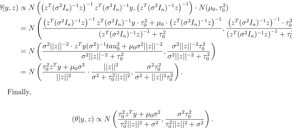
Recognizing that this expression is a convolution of two Gaussians with respect to θ,

(θ|y, z)∝N zT(σ2In)−1z

−1

zT(σ2In)−1y, zT(σ2In)−1z

−1

·N(µ0, τ02)

=N z

T₍_σ2_I

n)−1z

−1

zT₍_σ2_I

n)−1y·τ02+µ0· zT(σ2In)−1z

−1

(zT₍_σ2_I

n)−1z)

−1

+τ2 0

, z T₍_σ2_I

n)−1z

−1

·τ2 0

(zT₍_σ2_I

n)−1z)

−1

+τ2 0

!

=N

σ2_||_z_||−2_·_zT_y₍_σ2₎−1_tau2

0+µ0σ2||z||−2

σ2_||_z_||−2₊_τ2 0

, σ

2_||_z_||−2_τ2 0

σ2_||_z_||−2₊_τ2 0

=N

τ2

0zTy+µ0σ2

||z||2 ·

||z||2

σ2₊_τ2 0||z||2

, σ

2_τ2 0

σ2₊_||_z_||2_τ2 0

.

Finally,

(θ|y, z)∝N

τ2

0zTy+µ0σ2

τ2

0||z||2+σ2

, σ

2_τ2 0

τ2

0||z||2+σ2

.

Equipped with the full conditional distributions, the resulting Gibbs sampler is:

Initialize θ;

for t= 0 to T −1 do for i= 1 to n do

sample z_i(t) ∼N θyi θ2₊_σ2,

σ2

θ2₊_σ2

;

end

sample θ(t) _∼_Nτ2

0zTy+µ0σ2

τ2

0||z||2+σ2 ,

σ2_τ2 0

τ2

0||z||2+σ2

;

[image:38.612.78.545.319.524.2]

end

(39)

CHAPTER 3. GIBBS SAMPLING AND THE BAYESIAN FRAMEWORK 27

0.0 0.5 1.0

−10.0 −9.5 −9.0 −8.5

θ

[image:39.612.187.432.114.358.2]

Density

Figure 3.4: Empirical posterior distribution of theta

The posterior distribution for a sample of size n = 200 with σ2 _{= 1 is shown in Figure}

3.4. A data set of n = 200 observations were generated using θ = 10, σ2 _{= 1. The posterior}

is approximately normal-distributed as expected form the theoretical form of the posterior.

Maximuma posteriori estimates of θ using the empirical mean and median are -9.3757 and

-9.3411, respectively. The prior meanµ0 forθ was initialized toµ0 = 5 to see if the sampler

could recover the true θ with a biased prior. The posterior includes θ = 10 although the

influence of the prior is evident since the posterior distribution is centered above θ = 10.

Finally, inference on θ can be performed using a 95% Bayesian credible interval: (-9.7201,

-9.4612). The Bayesian credible interval does not contain θ = 10, which demonstrates the

(40)

CHAPTER 3. GIBBS SAMPLING AND THE BAYESIAN FRAMEWORK 28

3.6

A Gibbs Sampler for a Mixture of Two Gaussians

Next, consider a simple model for a continuous random variable and a discrete latent space.

SupposeY ∈_RwhereY is assumed to be generated by a mixture of two univariate Gaussians:

p(y;θ) =πφ y;µ1, σ12

+ (1−π)φ y;µ2, σ22

where θ= (π, µ1, µ2, σ12, σ22).

Assume that membership in the two Guassians is represented by a latent class variable

Z ∈ {0,1}where Z ∼Bernoulli(π)

p(zi) =πiz(1−π)1−zi, i∈[n]

and assume priors:

(π|η)∼Beta(η, η)

where π|η is a symmetric distribution center about π = 1₂,

(τk|αk, βk)∼Gamma(αk, βk)

where τk = _σ12

k is the precision and βk is the rate parameter for a gamma distribution,

(µk|τk, µ0k, νk)∼N µ0k,(νkτk)−1

where µ0k is the prior mean for µk and νk is the number of pseudo-observations used to

estimate µk. Note that it is assumed that the joint prior forµk and τk is

p(µk, τk) =p(µk|τk)·p(τk).

Finally, the forms of these prior distributions are given explicitly:

p(π|η) = Γ(2η) Γ(η)Γ(η)π

η−1₍₁₋_π₎η−1_{, π} _∈_[0_,_1]_{, η}_∈ R+.

p(τk|αk, βk) = βαk

k Γ(αk)

ταk−1

k exp{−βkτk}, τk, αk, βk∈R

(41)

CHAPTER 3. GIBBS SAMPLING AND THE BAYESIAN FRAMEWORK 29

p(µk|τk, µ0k, νk) = (2π)−

1 2 (ν

kτk)

1 2 exp

−1

2(µk−µ0k) (νkτk) (µk−µ0k)

.

The generative model can be represented as a graphical model as shown in 3.5

K = 2

N

K = 2

η νk µ0k αk βk

πk µk τk

zi

[image:41.612.172.441.194.436.2]

yi

Figure 3.5: Graphical model of a mixture of two Gaussians

In order to implement a Gibbs sampler to obtain the joint posterior distributionp(θ, z|y),

the full conditional distributions ofθandzi are needed. First, the full conditional distribution

of π is derived. Since z ∼ Bernoulli(π) and π ∼Beta(η, η), conjugacy will yield a posterior

where (π|z)∼Beta(·,·).

p(π|zi)∝p(zi|π)·p(π|η)

=πzi₍₁₋_π₎1−zi _·_πη−1₍₁₋_π₎η−1

(42)

CHAPTER 3. GIBBS SAMPLING AND THE BAYESIAN FRAMEWORK 30

It can be seen that the full conditional distribution of π is

(π|zi)∼Beta(zi+η,−zi+η+ 1).

Extending the result for π|zi to π|z,

p(π|z)∝p(π|η)· n

Y

i=1

p(zi|π)

=πη−1(1−π)η−1πPin=1zi₍₁₋_π₎n−Pni=1zi

=πn2+η−1₍₁₋_π₎n1+η−1_,

which yields

(π|z)∼Beta(n2+η, n1+η).

Next, the full conditional distribution of zi is derived:

p(zi|yi, θ)∝p(yi|zi, θ)·p(zi|π)

=

φ y;µ1, τ1−1

1−zi

φ y;µ2, τ2−1 zi

·πzi₍₁₋_π₎1−zi

p(zi|yi, θ)∝

(1−π)φ y;µ1, τ1−1

1−zi

πφ y;µ2, τ2−1 zi

.

Next, the full conditional distribution of τk is derived. Since ynk ∼ N(µk, τk) and τk ∼

Gamma(αk, βk), conjugacy will yield a posterior where (τk|ynk)∼Gamma(·,·):

p(τk|ynk, znk)∝ nk

Y

i=1

p(yi|zi, τk)·p(τk|αk, βk)

=τnk2

k exp ( −1 2 nk X i=1

(yi−µk)2τk

)

·ταk−1

k exp{−βkτk}

=τnk2 +αk−1

k exp ( − " 1 2 nk X i=1

(yi−µk)2+βk

#

τk

(43)

CHAPTER 3. GIBBS SAMPLING AND THE BAYESIAN FRAMEWORK 31

(τk|ynk, znk)∼Gamma αk+ nk

2 , βk+ 1 2

nk

X

i=1

(yi−µk)2

!

Finally, the full conditional distribution of µk is derived. Since ynk ∼ N(µk, τk) and

µk∼N(µ0k,(νkτk)−1), conjugacy will yield a posterior where (µk|ynk, τk)∼N(·,·).

p(µk|τk, ynk, znk)∝ nk

Y

i=1

p(yi|zi, µk, τk)·p(µk|τk, νk)

= exp ( −1 2 nk X i=1

(yi −µ2kτk)

)

·φ µk;µ0k,(νkτk)−1

= exp ( −1 2 nk X i=1

yiτkyi−2µkτk nk

X

i=1

yi+µknkτkµk

)

=φ µk; ¯ynk,(nkτk) −1

=φ µk;

¯

y_nk νkτk +

µ0k nkτk

1

nkτk +

1

νkτk ,

1

nkνkτk2

1

nkτk +

1

νkτk

!

=φ

µk;

nky¯nk+νkµ0k νk+nk

, 1 τk

· 1

νk+nk

(µk|τk, ynk, znk)∼N

nky¯nk +νkµ0k νk+nk

, 1 τk

· 1

νk+nk

(44)

CHAPTER 3. GIBBS SAMPLING AND THE BAYESIAN FRAMEWORK 32

Initialize πk, µk, τk,;

for t= 0 to T −1 do for i= 1 to n do

sample z_i(t+1) ∼

(1−π(t)₎_φ

y;µ(₁t), 1

τ1(t)

1−z_i(t)

π(t)_φ

y;µ(₂t), 1

τ2(t) z_i(t)

;

end

update group sizes n(₁t+1) and n(₂t+1) and group means ¯y₁(t+1) and ¯y(₂t+1); sample π(t+1) _∼_Beta(_n(t+1)

2 +η, n (t+1) 1 +η);

sample τ_k(t+1) ∼Gamma

αk+ n(_kt+1)

2 , βk+ 1 2

Pn (t+1)

k i=1

yi−µ(kt)

2

;

sample µ(_kt+1) ∼N

n_k(t+1)y¯_nk(t+1)+νkµ0k νk+n(_kt+1) ,

1

τ_k(t+1) ·

1

νk+n(_kt+1)

;

end

Figure 3.6: Gibbs sampler for mixture of two Gaussians

Data were generated by drawing 500 samples from N(µ1 =−10, σ2 = 9) and 500 samples

from N(µ2 = 10, σ2 = 9). Assuming that p(y;θ) = 0.5·φ(y;−10,32) + 0.5·φ(y; 10,32), a

sample of size n = 200 is generated after an initial burn-in period of 3000 iterations and

thinning every 15 samples to decorrelate the Markov chain. The following initializations

were used: µ01=−5, µ02 = 5, α1 =α2 = 1, β1 =β2 = 5, η = 0.5, ν1 =ν2 = 50.

The posterior distributions are shown in Figure 3.7. Note that all five posterior

distribu-tions are relatively symmetric and unimodal. Maximum a posteriori estimates using the

pos-terior means are: π = 0.4991, µ1 =−9.4976, τ1 = 0.1139,µ2 = 9.5430, τ2 = 0.1133. Finally,

inference onθcan be performed using 95% Bayesian credible interval: π: (0.4688,0.5293);µ1:

(−9.7475,−9.2362); τ1: (0.0989,0.1303); µ2: (9.3139,9.7757); τ1: (0.1013,0.1252). While

the Gibbs sampler is more complex than Algorithm 3.3, it successfully approximated the

(45)

CHAPTER 3. GIBBS SAMPLING AND THE BAYESIAN FRAMEWORK 33

µ2 τ2

µ1 τ1 π

9.2 9.4 9.6 9.8 0.10 0.11 0.12

−9.7 −9.5 −9.3 0.10 0.11 0.12 0.13 0.44 0.46 0.48 0.50 0.52 0.54 0

5 10 15 20 25

0 20 40 60

0 20 40 60 0

1 2 3

0 1 2 3

Parameter

[image:45.612.93.525.170.612.2]

Density

(46)

34

Chapter 4

Hidden Markov Models

4.1

The Generative Hidden Markov Model

The mixture model discussed in the previous chapter assumed that the latent variables

were mutually independent, an assumption that eases computation significantly. While

convenient, this assumption is not always reasonable. It is often more realistic in applications

such as speech processing (e.g. Levinson, Rabiner, and Sondhi 1983) to abandon probabilistic

models that rely on stationary distributions and instead attempt to model the non-stationary

nature of data directly. This is particularly useful in speech and text applications since

language is inherently temporal.

A hidden Markov model (HMM) assumes that randomly observed variables are generated

by an unobserved finite-state Markov chain. The observed random variables are assumed to

be generated by a different distribution for each latent state. More formally, a hidden Markov

model consists of a discrete-time process{(Xt, Yt)}, t= 0,1, . . . , T−1 whereXt denotes the

state of the latent Markov chain at time t, Yt denotes the observed value at time t, and T

values are observed. It is assumed that Yt depends onXt, but that Yt is independent of all

other latent values Xj, j 6=t. While it is theoretically possible to consider any configuration

(47)

CHAPTER 4. HIDDEN MARKOV MODELS 35

distribution of Yt|Xt can be discrete or continuous. For simplicity, only derivations for the

discrete case are considered. However, extensions to the continuous case are straightforward.

HMMs were first proposed in the literature in the 1960s (e.g. Baum and Petrie 1966) while

the EM algorithm for HMMs was proposed by Baum et al. (1970).

First, consider the discrete observations case. Suppose that there are N possible latent

states, X ∈ Q= {q0, q1, . . . , qN−1} and M possible observed values, Y ∈ {0,1, . . . , M −1}.

The Markov chain transitions from time t to time t+ 1 according to the N ×N transition

probability matrix

A={aij}

where aij =p(xt+1 =qj|xt =qi) and A is row stochastic such that Pjaij = 1, i= 1, . . . , N.

The initial state probabilities are

πx0 ={p(x0 =qj)}

where P

jπj = 1. Observations are generated according to the N ×M emission matrix

B ={bj(k)}

where bj(k) = p(yt=k|xt=qj),B is row stochastic, andk ∈ {0, . . . , M −1}.

The model λ = (π, A, B) fully define a discrete HMM and presents three distinct

prob-lems. First, it is of interest to determine the likelihood of a particular observed sequence

p(Y|λ). Second, one may seek to estimate the latent state sequence {X} that generated

the observed sequence {Y}. This problem can be solved using either the Viterbi algorithm

(Viterbi 1967) – which seeks the sequence{X∗}which maximizesp(X|Y, λ) – or the

forward-backward algorithm (Baum et al. 1970). Finally, estimation of the modelλcan be performed

(48)

CHAPTER 4. HIDDEN MARKOV MODELS 36

4.2

The Likelihood of the Discrete Hidden Markov

Model

Our main concern is in optimizing λ by maximizing the likelihood, so first consider the

process of obtaining the likelihood p(Y|λ) where Y = {y0, y1, . . . , yT−1} is the observed

sequence generated by the state sequence X ={x0, x1, . . . , xT−1}.

Since the observations are independent given xt,

p(Y|X, λ) = T

Y

t=0

p(yt|xt, λ).

By definition of the emission matrix B,

p(Y|X, λ) = bx0(y0)·bx1(y1)· · ·bxT−1(yT−1).

Next, note that using the definition of conditional probability,

p(Y|X, λ) = p(Y, X|λ) p(X|λ)

can be rearranged to obtain

p(Y, X|λ) =p(Y|X, λ)·p(X|λ).

Using the definitions of π and A,

p(X|λ) = p(x0|λ)·p(x1|x0, λ)· · ·p(xT−1|xT−2, λ)

=πx0 ·ax0,x1· · ·axT−2,xT−1.

Therefore,

p(Y, X|λ) =p(Y|X, λ)·p(X|λ)

(49)

CHAPTER 4. HIDDEN MARKOV MODELS 37

Summing over the latent space,

p(Y|λ) = X X∈X

p(Y|X, λ)·p(X|λ)

= X

X∈X

bx0(y0)·bx1(y1)· · ·bxT−1(yT−1)·πx0 ·ax0,x1· · ·axT−2,xT−1

= X

X∈X

πx0 ·bx0(y0)ax0,x1 ·bx1(y1)· · ·axT−2,xT−1bxT−1(yT−1).

Unfortunately, computing the likelihood in this manner requires approximately 2T NT

multiplications (Rabiner 1989). This becomes computationally prohibitive when the number

of observations T and states N grows large.

4.3

The Forward-Backward Algorithm

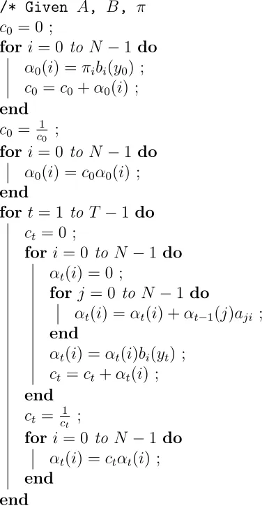
One attractive feature of the HMM is the forward-backward algorithm of Baum et al. (1970)

which makes the computation of the likelihood and the most probable latent state sequence

much faster. Next, the forward algorithm (one half of the forward-backward algorithm) for

determining the likelihood p(Y|λ) is defined. Define αt(i) = p(y0, y1,· · · , yt, xt = qi|λ) for

t= 0,1,· · · , T−1 andi= 0,1,· · · , N−1 as the joint probability of the observation sequence

up to timet and the latent state at time t. Let αt(i) denote the forward variable for time t.

αt(i) can be obtained inductively:

1. α0(i) =πi·bi(y0), i= 0,1,· · · , N −1

2. αt+1(j) = h

PN

i=1αt−1(j)aij

i

bj(yt),1≤t ≤T −1,0≤, j ≤N−1

3. p(Y|λ) =PN−1

i=0 αT−1(i).

(50)

CHAPTER 4. HIDDEN MARKOV MODELS 38

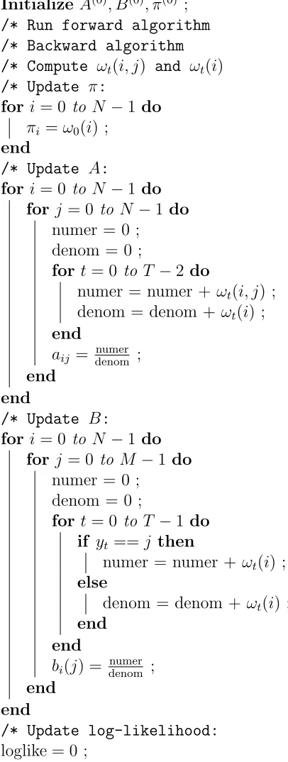
/* Given A, B, π */

c0 = 0 ;

for i= 0 to N −1 do

α0(i) = πibi(y0) ;

c0 =c0+α0(i) ; end

c0 = _c1₀ ;

α0(i) = c0α0(i) ; end

for t= 1 to T −1 do

ct= 0 ;

αt(i) = 0 ;

for j = 0 to N−1 do

αt(i) = αt(i) +αt−1(j)aji ;

end

αt(i) =αt(i)bi(yt) ; ct=ct+αt(i) ;

end

ct= _c1_t ;

αt(i) =ctαt(i) ;

[image:50.612.90.283.116.480.2]

end end

Figure 4.1: Forward algorithm

Instead of the naive direct computation of the likelihood’s required 2T NT _{multiplications,}

the forward algorithm only involves approximatelyN2_T _{multiplications. While this will still}

take longer to compute as N and T increase, it is much faster.

The second half of the forward-backward algorithm yields the backward variable βt(i)

which is defined as

β(i) = p(yt+1, yt+2, . . . , yT−1|xt=qi, λ).

Like the forward variables, the backward variables can be computed inductively:

(51)

CHAPTER 4. HIDDEN MARKOV MODELS 39

2. βt(i) =PN

−1

j=0 aijbj(yt+1)βt+1(j), t=T −2, T −3, . . . ,0, i= 0,1, . . . , N −1.

An algorithm for computing the backward variables is given in Figure 4.2.

/* Given A, B, π */

βT−1(i) = cT−1 ; end

for t=T −2 to 0 do for i= 0 to N −1 do

βt(i) = 0 ;

for j = 0 to N−1 do

βt(i) = βt(i) +aijbj(yt+1βt+1(j) ; end

βt(i

Bayesian Hidden Topic Markov Models

Rochester Institute of Technology

Contents

List of Figures

List of Tables

Chapter 1

Overview

CHAPTER 1. INTRODUCTION 2

CHAPTER 1. INTRODUCTION 3

Organization

CHAPTER 1. INTRODUCTION 4

Chapter 2

CHAPTER 2. RELATED WORK 6

Latent Semantic Indexing

Probabilistic Latent Semantic Indexing

CHAPTER 2. RELATED WORK 8

Latent Dirichlet Allocation

CHAPTER 2. RELATED WORK 9

CHAPTER 2. RELATED WORK 10

CHAPTER 2. RELATED WORK 11

CHAPTER 2. RELATED WORK 12

Departures from the “Bag-of-Words” Assumption

CHAPTER 2. RELATED WORK 13

Correlated Topic Modeling

CHAPTER 2. RELATED WORK 14

Dynamic Topic Modeling

CHAPTER 2. RELATED WORK 15

Hidden Topic Markov Modeling

CHAPTER 2. RELATED WORK 16

CHAPTER 2. RELATED WORK 17

CHAPTER 2. RELATED WORK 18

Chapter 3

CHAPTER 3. GIBBS SAMPLING AND THE BAYESIAN FRAMEWORK 20

CHAPTER 3. GIBBS SAMPLING AND THE BAYESIAN FRAMEWORK 21

Markov Chain Monte Carlo

Metropolis-Hastings Algorithm

CHAPTER 3. GIBBS SAMPLING AND THE BAYESIAN FRAMEWORK 22

CHAPTER 3. GIBBS SAMPLING AND THE BAYESIAN FRAMEWORK 23

Gibbs Sampling

CHAPTER 3. GIBBS SAMPLING AND THE BAYESIAN FRAMEWORK 24

A Gibbs Sampler for a Univariate Latent Variable

CHAPTER 3. GIBBS SAMPLING AND THE BAYESIAN FRAMEWORK 25

CHAPTER 3. GIBBS SAMPLING AND THE BAYESIAN FRAMEWORK 26

CHAPTER 3. GIBBS SAMPLING AND THE BAYESIAN FRAMEWORK 27

CHAPTER 3. GIBBS SAMPLING AND THE BAYESIAN FRAMEWORK 28

A Gibbs Sampler for a Mixture of Two Gaussians

CHAPTER 3. GIBBS SAMPLING AND THE BAYESIAN FRAMEWORK 29

CHAPTER 3. GIBBS SAMPLING AND THE BAYESIAN FRAMEWORK 30

CHAPTER 3. GIBBS SAMPLING AND THE BAYESIAN FRAMEWORK 31

CHAPTER 3. GIBBS SAMPLING AND THE BAYESIAN FRAMEWORK 33

Chapter 4

CHAPTER 4. HIDDEN MARKOV MODELS 35

CHAPTER 4. HIDDEN MARKOV MODELS 36

The Likelihood of the Discrete Hidden Markov

CHAPTER 4. HIDDEN MARKOV MODELS 37

The Forward-Backward Algorithm

CHAPTER 4. HIDDEN MARKOV MODELS 38

CHAPTER 4. HIDDEN MARKOV MODELS 39