Study of Damage Progression In CSCM Concretes Under Repeated Impacts

Rochester Institute of Technology

RIT Scholar Works

Theses Thesis/Dissertation Collections

4-21-2017

Study of Damage Progression In CSCM Concretes

Under Repeated Impacts

Yevgeniy Parfilko [email protected]

Follow this and additional works at:http://scholarworks.rit.edu/theses

This Thesis is brought to you for free and open access by the Thesis/Dissertation Collections at RIT Scholar Works. It has been accepted for inclusion in Theses by an authorized administrator of RIT Scholar Works. For more information, please [email protected].

Recommended Citation

Rochester Institute of Technology

Study of Damage Progression In

CSCM Concretes Under Repeated Impacts

A Thesis

Submitted in Partial Fulfillment of the Requirements

for the Degree of Master of Science in Mechanical Engineering

In the Department of Mechanical Engineering

Kate Gleason College of Engineering

By

Yevgeniy Parfilko

DEPARTMENT OF MECHANICAL ENGINEERING

KATE GLEASON COLLEGE OF ENGINEERING

ROCHESTER INSTITUTE OF TECHNOLOGY

ROCHESTER NEW YORK

CETIFICATE OF APPROVAL

M.S. DEGREE THESIS

The M.S. Degree Thesis of Yevgeniy Parfilko has been examined

and approved by the thesis committee as satisfactory for the

thesis requirement of Master of Science Degree.

Approved by:

___________________________________________________

Dr. Benjamin Varela, Advisor, RIT Dept. of Mechanical Engineering

___________________________________________________

Dr. Hany Ghoneim, Committee Member, RIT Dept. of Mechanical Engineering

___________________________________________________

Dr. Sarilyn Ivancic, Committee Member, RIT Dept. of Mechanical Engineering

___________________________________________________

Abstract

Reinforced Concrete (RC) is an important material in civil construction projects, and rigorous standards exist for rating the structural, wind, vibration, and cyclic design loads. In narrower applications, such as the design of protective saferooms, RC is also designed to bear impact loads which may be applied repeatedly. Although current experimental and computational methods allow for prediction of concrete damage from a single impact, there is no attempted study of damage progression from repeated impacts. Such a study is attempted on a well-defined slab impact test used in the rating of protection provided by RC walls. Multiple projectiles impact a chosen location and accumulating damage is predicted by means of numerical simulation. The simulation results are then correlated to an experimental test demonstrating similar effects.

The classic projectile impact problem is taken as the basis for computational analysis. Nonlinear wood and concrete material models are substituted for the conventional steel projectile and target, and a damage variable is defined to track cumulative effects of plastic strain. The

simulation is then extended to additional impacts while preserving the damaged state of the slab. The development of damage and accumulating strain energy is computed, until damage extends throughout the entire thickness of the slab. Since the contact period per impact is estimated to be under a millisecond, an explicit dynamics formulation of the problem is implemented in

commercial software LS-DYNA. The concrete stresses are computed using the Reidel-Hermaier-Thoma Model (RHT), which incorporates a smooth geologic cap model to provide a single continuous failure surface. In this manner, compaction, shear and tensile failures are represented, and consolidated for post-processing by means of a single damage variable.

To verify computational predictions, the impact is recreated experimentally. A set of wood projectiles and RC slabs are fabricated, to allow for repeatable tests. Initial and boundary conditions are recreated by means of a steel bracket for the slab and an air cannon for the

projectile. After initial calibration, a repeatable projectile speed, impact location and momentum transfer is achieved. The slabs are impacted repeatedly until macroscopic damage is clearly visible on the front and back faces of the slab. Damaged slabs are then cross-sectioned for material failures and plastic deformation.

Acknowledgements

I would like to extend my gratitude to my advising committee, who have been invaluable

mentors to me during this rewarding journey. Dr. Benjamin Varela, Dr. Hany Ghoneim and Dr.

Sarilyn Ivancic have provided guidance, patience, and instruction without which this work would

not have been possible. Additional thanks goes out to RIT faculty Stephen Boedo and Timothy

Landschoot, who have assisted greatly by offering their consultations and lending test

equipment. Last but not least, I extend sincerest gratitude to William Finch, Paul Mezzanini,

Diane Selleck, Jan Maneti, Rob Kraynik, Kathleen Ellis, and Fernando Amaral de Arruda, for

their unwavering support of my efforts, and for transforming the academic environment into a

warm, welcoming family. For their love, caring, and years of support, a special thanks goes to

my parents Oksana and Vadim, who have given me the motivation and the means to pursue my

Table of Contents

Abstract . . . 2

Table of Contents . . . 4

List of Figures . . . 6

List of Equations . . . 7

List of Tables . . . 7

Terminology . . . 8

1.0Introduction . . . 9

1.1Societal Context . . . 12

1.2Research Objectives . . . 13

1.3Scope of this work . . . 14

2.0Literature Review . . . 15

2.1A history of concrete design for ballistic impacts . . . 15

2.1.1 Early military applications . . . 15

2.1.2 Civil applications . . . 18

2.1.3 Modern applications . . . 20

2.2A history of computational analysis of impacts . . . 21

2.2.1 Concrete material models . . . 23

2.3Experimental Failure Modes . . . 28

3.0Methodology . . . 31

3.1Experimental Design . . . 31

3.2Simulation Methodology . . . 34

3.2.1 Preliminary work . . . 34

3.2.2 Geometry . . . 39

3.2.3 Mesh . . . 40

3.2.4 Material Models . . . 40

3.2.5 Contact Formulation . . . 41

3.2.6 Timescale . . . 41

3.3Experimental Methodology . . . 43

3.3.1 Projectile . . . 43

3.3.2 Concrete slab . . . 43

3.3.3 Air cannon . . . 44

3.3.4 System calibration . . . 44

3.3.5 Data acquisition . . . 44

3.3.6 Test procedure . . . 45

4.0Results and Discussion . . . 46

4.1Simulation Overview . . . 46

4.2Single Impact Results . . . 46

4.2.1 Part energies . . . 49

4.2.2 Stresses and strains . . . 49

4.2.3 Nodal displacements and accelerations . . . 51

4.2.4 Damage verification . . . 52

4.3Repeated Impact Results . . . 53

4.3.1 Slab energies . . . 53

4.3.2 Strain and damage accumulation . . . 54

4.4Experimental Results . . . 56

4.4.1 Concrete strength and properties . . . 56

4.4.2 Air cannon tests . . . 56

4.4.3 Accelerometer data . . . 57

4.4.4 Observed failure modes . . . 58

5.0Conclusions and Future Work . . . 60

6.0Bibliography . . . 62

7.0Appendices . . . 65

7.1Appendix A: Drawing of Experimental Setup . . . 65

List of Figures

Figure 2.1 Example 3-D problem solved by DYNA-3D . . . 22

Figure 2.2 Limit surface of MAT_PSEUDO_TENSOR . . . 23

Figure 2.3 Geologic Cap Model by Sandler and Rubin . . . 24

Figure 2.4 Continuous Surface Cap as used in MAT_CSCM . . . 26

Figure 2.5 Four common failure modes of concrete . . . 29

Figure 3.1 Visualization of preliminary impact simulation . . . 34

Figure 3.2 Visualization of plastic strain in model cross section . . . 35

Figure 3.3 Acceleration nodal histories for the preliminary impact simulation . . 36

Figure 3.4 Penetration depth at various simulated environmental conditions . . . . 37

Figure 3.5 Velocity-dependent penetration predictions for soft missiles . . . 38

Figure 3.6 Corner impact test visualizations . . . 39

Figure 3.7 Illustration of the simulation model and mesh . . . 40

Figure 3.8 Schematic of test setup and equipment . . . 43

Figure 3.9 Schematic of the data signal path . . . 45

Figure 4.1 Energy component time histories of the slab and projectile . . . 47

Figure 4.2 Cross section of the slab after impact, showing subsurface damage . . 48

Figure 4.3 Comparison of pressure, plastic strain and residual shear stress . . . 49

Figure 4.4 Time history of acceleration and displacement . . . 50

Figure 4.5 Energy component time histories of the repeatedly impacted slab . . . 52

Figure 4.6 Visualization of the slab damage over 4 impacts . . . 53

Figure 4.7 Back face of the slab, showing four radial crack regions . . . 54

Figure 4.8 Raw and processed images of slab #2 after the second impact . . . 56

Figure 4.9 Accelerometer data and power spectrum response from test #1 . . . 56

Figure 4.10 Digitally marked images of slab #2 impact test . . . 57

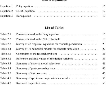
List of Equations

Equation 1 Petry equation . . . 16

Equation 2 NDRC equation . . . 17

Equation 3 Kar equation . . . 19

List of Tables

Table 2.2 Parameters used in the NDRC formula . . . 18

Table 2.3 Survey of 27 empirical equations for concrete penetration . . . 20

Table 2.4 Survey of 19 numerical models for concrete simulation . . . 27

Table 3.1 Constraints of the research problem . . . 31

Table 3.2 Reference and final values of the design variables . . . 33

Table 3.3 Summary of material model selections . . . 41

Table 3.4 Summary of post-processing steps . . . 42

Table 3.5 Summary of test procedure . . . 45

Table 4.1 Summary of specimen compression test results . . . 55

Terminology

ASTM American Society for Testing and Materials

NSSA National Storm Shelter Association

NDRC National Defense Research Committee

ACE Army Corps of Engineers

CEA Commissariat à l’Energie Atomique

UKAEA United Kingdom Atomic Energy Authority

BRL Ballistic Research Laboratory

LLNL Lawrence Livermore National Laboratory

LSTC Livermore Software Technology Company

RC Reinforced concrete

ED Explicit Dynamics

FEM / FEA Finite Element Method / Analysis

APDL ANSYS Parametric Design Language

FFT Fat Fourier Transform

MIC Multiple Impact Condition

RHT Riedel-Hermaier-Thoma [Concrete Material Model]

CSCM Continuous Surface Cap Model

𝑓_𝑐′ _{= unconfined compressive strengthof concrete in psi}

𝑉₀ = initial impact velocity in ft/s

𝐷 = damage scaling factor

𝑑 = missile diameter in inches

𝑁 = missile nose cone shape factor

E = elastic modulus in psi

Em = elastic modulus of mild steel in psi

W = missile or projectile weight

x = penetration depth

1.0

Introduction

Concrete is a hard, brittle material that is present in a variety of structures. It is the oldest

engineered structural material, and the first to be used on a large scale in civil construction.

Concrete is composed of a hardening cement and a space-filling aggregate. It is known for being

a dense, monolithic material that is strong in compression and weaker in tension.

The basic principle of a cement is a hydraulic setting compound, meaning that the cement reacts

with water and produces mineral hydrates that act as a binder. Lime, calcium silicate, fly ash, and

other mineral compounds can be combined and used as cements. The aggregate that is bound by

the cement may be any available material with desirable properties. Sand and gravel are used for

construction-grade concrete, while glass, foam or other industrial materials may be used to

produce lightweight, heat-resistant, or environmentally friendly concretes. The flexibility of

composition results in a range of properties for a wide array of applications, but the mechanical

properties of concrete in construction are of primary interest.

The first widespread application of concrete where it was the primary material was the pouring

of a load-bearing arch, allowing continuous loading over a span with a discrete number of

supports [19]. Domes were an extension of the arch that allowed for the construction of covered

buildings and are geometrically complex enough that the use of concrete over worked stone was

justified. Additionally, arches had the advantage of creating a purely compressive stress field,

thus avoiding concrete’s weaker tensile properties.

Cement was manufactured locally and in small batches, with its chemical composition varying

by location. Thus its properties were not significantly repeatable like those of metallic materials.

century, and materials such as Portland cement became common enough to allow a standard of

comparison for mechanical properties. The first use of these new concretes was in the laying of

foundations for lighthouses on rocky cliffs, where conventional foundations were impossible to

construct.

As concrete became more readily available, its uses expanded to a variety of fields, allowing for

further innovation. Concrete reinforcement technology was developed in France in the 19th

century. Joseph Monier, for example, filed patents for reinforced concrete pipes, beams and

bridges between 1868-1878 [19], and his ideas were backed up with engineering data published

by Gustav Adolf Wayss. Now that concrete with repeatable properties could be produced and its

bearing loads calculated, European engineers began to design bridges, dams and forts with

concrete as the primary material.

A common metric to determine the rated strength of concrete is to observe its maximum

compressive load in a uniaxial compression test. Today, 2-inch cubes or various size cylinders,

as described in the ASTM C109 standard, are used [1]. From the load and geometry, an estimate

of the average compressive stress may be obtained, with typical concretes having a strength of

20-35 MPa. The tests, however, do not show the compaction strength of concrete, since the

specimen will first fail in tension resulting from the deformation of its free surfaces.

Although buildings such as the roman Pantheon have been known to maintain structural integrity

for over 18 centuries, concrete structures that are subjected to impacts and excessive vibrations

are at a constant risk of brittle failure. To extend the safety of concrete structures and range of

application for concrete, advancements were sought in composites and material science.

over properties such as viscosity, settling time, and susceptibility to corrosives. Modern

ultrasonic and laser measurement methods enable preventative maintenance, reducing failures

greatly. In the present day, concrete is a much more robust material both in terms of load-bearing

capability and performance in adverse environmental conditions.

Engineering efforts to completely characterize the mechanics of concrete materials is ongoing.

Unlike metals, concretes exhibit complex behavior under strain, including rate-dependent linear

deformation, nonlinear plastic deformation, and a variety of fracture modes. The mechanical

behavior of concrete was not rigorously quantified until the mid-twentieth century, and various

properties such as flame resistance and ecological impact are still being studied in the

engineering theory of concretes. These properties are important to consider because they allow

the feasibility of concrete application in various unconventional scenarios. Thermal properties of

concrete dominate in design of rocket launch pads, for instance, while mechanical fracture is an

important consideration for any protective structures or vehicle-related construction. A thorough

understanding of these properties is necessary to extend the performance predictions of the

structure through its anticipated lifetime.

This work is concerned with a particular type of concrete failure, occurring due to accumulated

damage from impacts. This phenomenon, called a multiple impact condition, occurs when an

impact load causes localized damage to the concrete, and compounds existing damage from a

previous, untreated impact. Section 1.2, research objectives, explains in detail what properties

1.1 Societal Context

Reinforced concrete found widespread use in civil applications of roads, bridges, dams, docks,

canals and protective walls or traffic barriers. Protective structures commonly utilize some form

of reinforced concrete. As a consequence of its long lifespan, concrete is expected to protect

against many instances of damage, including crashes or ballistic impacts.

Proper characterization of concrete damage and its effect on the service life of concrete is crucial

to engineers that set design and maintenance goals for the structure. Understanding the dynamic

behavior of concrete materials under impact will result in better-designed structures, which will

in turn minimize civilian injuries. Similarly, understanding the damage progression in concrete

will result in better assessment of damage zones after the impact has taken place.

As performance and rigor of design continue to increase, proven design paradigms may be

incorporated into codes and standards that guide the development of future projects. At the

present time, additional research work will be necessary in order for the standards to be

1.2

Research Objectives

The primary research question is to characterize the repeated impact phenomenon. Since repeated

impacts have not been studied from a perspective of structural codes and standards, several

derivative implications are to be considered in addition to the main research question:

 What are the transient dynamics of a missile impact into pre-damaged concrete?

Specifically, what are the stresses, strains, contact pressures, and accelerations of

material elements within the immediate impact zone? How do finite element

predictions compare to experimental data?

 Can existing empirical and numerical models in published literature be extended to

predict accumulating damage from repeated impacts? If they can, how accurate are

the predictions relative to the prediction from initial impact? If they cannot, how

may an accurate prediction model be constructed from experimental data?

 How can the insight into behavior of pre-damaged concrete be incorporated into

safety standards to make them more comprehensive? Can a structure be designed

to withstand a minimum number of consecutive impacts rather than a single

impact? Alternatively, can a non-intrusive inspection be used to determine a repair

procedure to return structural integrity, given a period of potential exposure?

In order to answer the research question, itemized objectives are set forth to allow the study, data

collection, analysis and review of the repeated concrete impact experiments. The following

section lays out the format of this work and describes how each section supports the

1.3 Scope of the Present Work

 To study the transient dynamics of a missile impact into pre-damaged concrete, a robust,

efficient finite element model is developed. The model consists of one or more impacting

masses and a constrained concrete specimen. Stress, strain, contact pressure, and local

accelerations in the impact zone will be simulated.

 The design and characterization of the experimental setup will be conducted based on the

predicted results of the finite element simulation. The type, quantity and placement of

proper sensing equipment will be derived from the computational model, to allow

analogous data to be collected. The initial conditions will be supplied by a projectile

acceleration system, and the boundary conditions will be met by means of a rigid support.

 The experimental setup and proper measuring equipment will be fabricated in four

sections: an air cannon to launch and measure the speed of soft projectiles, a set of

concrete slabs with accelerometers, a set of projectiles, and a constraining bracket. The

experimental setup will be designed to be reusable, except for the concrete specimens.

 Experimental tests will be executed to replicate and validate the simulations. Acceleration

data will be recorder in real time, and the concrete material will be inspected after each

impact to obtain plastic deformation and damage measurements. The geometry of the

cracks will be measured and compared to previous instances to infer the propagation.

 The data obtained from experiment will be compared to numerical models, and if

possible, fit to the respective model parameters to show how repeated impacts relate to

2.0

Literature Review

Over the 150 years since the industrial revolution, concrete has been used for industrial,

defensive, aesthetic and commercial projects on a variety of scales. During this time, analytical

methods, design standards, and experimental tests for concrete structures underwent significant

changes. The progression of these methods within the context of application will be summarized

thoroughly and concisely in the literature review section.

2.1 A history of concrete design for ballistic impacts

2.1.1 Early military applications

Concrete, along with other forms of masonry, has been used in a variety of structures ranging

from aqueducts to temples to protective walls. These historic structures were designed to bear a

static load, most of which was the material weight. Transient loads were addressed by

incorporating a large factor of safety. Thus, the primary engineering effort was to ensure the

structure could support its initial load. The first consideration of external impact loading

stemmed from the problem of designing an economical protective military structure to be able to

withstand the transient load from a ballistic projectile. Initial work specifically addressed

dull-nosed steel artillery shells. However, the strength of the pour depended heavily on the quality of

the cement and the workmanship; the strength of a structural pour was not yet repeatable.

In the beginning of the twentieth century, concrete technology had developed enough to allow

large-scale civil engineering projects. The first publication to rely on experimental data in

quantifying the protection provided by a barrier was conducted by Petry in 1910 [26]. Petry

assumed a solid steel projectile and a semi-infinite concrete barrier, such that the missile could

𝑋 = 12 𝐾_𝑝𝐴_𝑝log₁₀(1 + 𝑉0 2

215000_{𝑓𝑡/𝑠})

Equation 1. Petry I equation as given by Amirikian [4].

Based on ballistic impact tests, Petry was able to establish a logarithmic correlation of the kinetic

energy of the projectile (given by the squared velocity term, and normalized to a reference

velocity) to the relative depth of penetration (given by X). Linear constants Ap and Kp allowed

the prediction to account for the frontal weight-per-area of the missile and material property

constant of the concrete, respectively. Table 2.1 shows each variable, its description and units.

Table 2.1. Input/output parameters for the Petry equation [13].

Variable name Symbol Units Ref. value

Depth of penetration X ft 0.0100

Concrete material penetration coefficient Kp - 0.0083 Missile weight per projected area Ap lb/ft2 ₆₀₀

Impact velocity Vo ft/s 450

This equation was not dimensionally accurate, and was a simple fit of a logarithmic law to test

data; the corresponding report was published as a “Monograph on Artillery Systems” [26]. Not

surprisingly, little academic progress was made over the next forty years, and the next landmark

work to be published in the field was authored by U.S. naval head design engineer Arsham

Amirikian in 1950 [6]. Amirikian references the work of Petry, and derives a graphical

representation of the Petry equation. However, he writes in his report, “Design of Protective

Structures”, that determining penetration depth beyond a rough estimate is of little practical

interest due to the variety of factors that control impact speed and force. Rather than offering a

single equation for concrete barriers, Amirikian introduces several approximations for solid

missile impacts and various blast loads, and bases the concrete dimensions on heuristic estimates

of a factor of thickness. For instance, he illustrates that for a 2,000 lb. explosive charge

to the explosion energy and 3.15 feet due to the kinetic energy. He then suggests a design with a

double ceiling of 6 feet and 4 feet, respectively, to absorb the two energies independently. This

type of estimation is consistent with the conservative design philosophy employed by military

engineers, where there was a continued risk of weapons technology advancing unexpectedly. The

recommendation also shows that protective structures of the time were designed to withstand a

single, head-on impact and did not make any provisions for the assessment of damage and

ultimate repair of the construction.

Meanwhile, in the 1940s the National Defense Research Committee was tasked with conducting

extensive experimental tests to determine the penetration capabilities of more modern ballistic

missiles, which were known to reach speeds up to 3000 m/s. Data sets from about 900 missile

tests were subsequently summarized by curve-fit equations, and are generally known as the

NDRC equations [13]. They became widely used in the 1950s due to their closed form and

straightforward simplicity. Rather than relying on precise missile characterization, the NDRC

equations made up for unforeseen parameter variation by giving conservative estimates of

required concrete thickness.

𝐺 (𝑥 𝑑) =

180

(𝑓_𝑐′)0.5 𝑁 𝐷 𝑑0.2( 𝑉0 1000)

1.8

; 𝐺 (𝑥 𝑑) = {

(𝑥

2𝑑)

2 _𝑓𝑜𝑟 𝑥 𝑑< 2 𝑥

𝑑−1 𝑓𝑜𝑟

𝑥 𝑑≥2

Equation 2. NDRC equations as given by Teland [30].

The equation differs from the Petry equation in several respects. Most notably, the compressive

strength of the concrete is a direct input parameter rather than the specific weight constant used

by Petry. The equation also considers two cases of penetration, described by the function G(x/d).

In one case, the penetration depth is less than twice the projectile diameter, and in the other case

that time. The non-integer exponents of the equation are the result of statistical regression

methods that were used estimate the parameters based on the test data. A description of the

equation variables is given in Table 2.2.

Table 2.2. Input/output parameters for the NDRC and Kar equations. [13].

Variable name Symbol Units Ref. value

Normalized depth of penetration x/d ft./ft.

Concrete compressive strength fc' psi 3000

Nose cone shape factor N - 1.0

Missile weight W lb. 50.0

Missile diameter D in. 4.0

Impact velocity Vo ft/s 450

Elasticity ratio (material to mild steel) E/Em psi/psi 1.0

To summarize, various military engineers laid the groundwork for evaluating concrete impacts.

Perty introduced the method of impact testing, while Amirikian was able to derive some general

guidelines for estimating impact loads based on missile parameters. The NDRC was able to

supply more extensive test data and a more refined set of formulas. Despite these improvements,

the scope of the work was narrowly focused on the design of bunkers and missiles, with no

consideration for repair or extended service life.

2.1.2 Civil Applications

In the years after the Second World War, design considerations shifted away from preventing

missile penetration, and focused on civil applications. Rapid growth of suburbs created an

enormous demand for concrete in roadways, bridges, dykes, tunnels and barriers. Energy

infrastructure hubs such as power plants still needed protective enclosures however, and these

were now required to serve a much longer life. These structures needed to be economical and

withstand multiple modes of failure – scabbing, spalling, weathering – instead of simply lasting

This trend was reflected in the research on concrete, as witnessed by several studies into

optimizing concrete designs. Since concrete structures were now designed to last decades rather

than months, more subtle forms of wear and weathering were being taken into account.

Consulting engineer A. K. Kar [17], for instance, conducted a comparative study on the effect of

softer, lighter projectiles into concrete structures, such as those imparted by tornado-accelerated

debris. He implemented a modified NDRC formula and included a term to scale the penetration

depth of projectiles based on their elastic modulus relative to mild steel.

𝐺 (𝑥 𝑑) =

180 (𝑓_𝑐′)0.5 (

𝐸 𝐸_𝑚)

1.25 _{𝑊 𝑁}

2 𝐷 𝑑1.8(

𝑉0 1000)

1.8

; 𝐺 (𝑥 𝑑) = {

(𝑥

2𝑑)2 𝑓𝑜𝑟 𝑥 𝑑< 2 𝑥

𝑑−1 𝑓𝑜𝑟

𝑥 𝑑≥2

Equation 3. Kar Formula for penetration from tornado-generated missiles [30].

The Kar equation has the same proportional relationships as the NDRC equation, and makes the

additional assumption that penetration from projectiles less dense than steel will scale according

to a power law. The significance of this term is that, in addition to allowing a missile of any

material, the analyst might now be able to derive an elastic modulus of a composite assembly,

such as a vehicle. Studies conducted by engineers such as Kar generated a fair amount of

experimental data on concrete impacts, and gave concrete manufacturers, as well as structural

engineers, access to a variety of simple, closed-form formulas that accelerated design

calculations. A majority of these formulas were developed from 1975 to 1999; a selection of

formulas and their years of publication is given in Table 2.3. Although they were simple to use,

researchers developed them independently and with regard to a specific applications or datasets.

Thus, the use of multiple formulas when designing for complex failure conditions was not

practical, as the penetration predictions for each formula varied substantially. A certain degree of

intuition was required to know which formula would best match an experimental application, as

Table 2.3. Summary of published formulas to predict missile penetration into concrete or geopolymer materials [30].

Formula Name Pub. Yr. Purpose

Army Corps of Engineers Formula 1946 Military & civil construction Adeli and Amin Formula 1984 Best polynomial fit

Ammann and Whitney Formula 1976 Explosive fragments Bechtel Corporation Formula 1976 Scabbing prediction

Bergman Formula 1949 Based on Beth formula

British Formula 1988 Weapons penetration

Ballistic Research Lab Formula 1969 Perforation – ballistics CEA-EDF Formula for Perforation 1977 Perforation – nuclear reactor

Chang Formula 1981 Perforation and scabbing

CKW-BRL Formula 1982 Semi-infinite targets

Forrestal Formula 1994 Semi-analytical derivation

Haldar and Miller Formula 1982 Nuclear reactor protection

Hughes Formula 1984 Neglects scabbing/perforation

IRS Formula 1984 Crater prediction

Kar Formula 1978 Tornado generated missiles

Kar Steel Target Formula 1968 Low velocity impacts McMahon, Meyers and Sen Model 1979 Soft Impacts

Barr, Carter, Howe, and Nielson Formula 1980 Structural impact

Modified NDRC Formula 1946 Ballistic missile penetration

Petry Equation 1910 Projectile penetration

Perry and Brown Formula 1982 Pre-stressed slabs

Stone and Webster Formula 1976 Scabbing

Takeda, Tachikawa and Fujimoto Formula 1979 Hard impacts

British Textbook of Air Armament Form. 1955 Aggregate size dependence Tolch and Bushkovich Formula 1947 Penetration into rock

UKAEA Formula 1990 Nuclear reactor protection

Young Formula 1996 Penetration mechanics course

2.1.3 Modern applications

Today, certain protective structures continue to be designed to prevent penetration of various

projectiles. Government buildings and nuclear fuel storage facilities, for instance, are often

designed to withstand commercial airplane crashes [16]. Roadside barriers and various

transportation-related structures are designed to withstand a glancing vehicle collisions [21] [5].

Tornado saferooms are designed to protect against debris, wind, or falling trees [24] [25].

Due to the varied nature of the scale, geometry, and environmental conditions of these problems,

application. Instead, the structural soundness is verified by commercial and proprietary finite

element programs, and empirical equations are only used to set bounds for design parameters.

The advantage to the use of finite element models over empirical equations is that only local

failure of any given element is considered, and the global depth of damage or penetration is a

result of running a simulation with the desired mesh and initial conditions. In this way, damage

on surfaces with non-standard boundary conditions may be found, or missiles with non-standard

geometry may be studied. The main disadvantage of this method is the computational cost.

2.2 A history of computational analysis of impacts

Weapons technology advanced significantly during the cold war era, and the proliferation of

nuclear missiles introduced a completely new set of defense criteria. Rather than dissipating the

momentum from a point load, a concrete shelter could now be subjected to a propagating

shockwave. This necessitated an analysis technique known as explicit dynamics, where the

dynamic state of a system is solved for by numerical extrapolation over a small time step.

Because this technique used a discretized time domain, it made sense to use a discretized spatial

domain as well, in the form of a finite element formulation of the dynamic system.

The first research organization to achieve an explicit dynamics solver for 3-D finite element

problems was the Lawrence Livermore National Laboratory (LLNL). A solver called

DYNA-3D, written by Dr. John O. Hallquist [15] in 1976, was used for the assessment of the

effectiveness of atomic weapons systems. It was also the first 3-D FEA solver to incorporate

general single surface contact [8]. Later development of DYNA-3D focused on computational

efficiency of elements and advanced material models for the medical, automotive and aerospace

and DYNA-3D became the commercial code LS-DYNA. Figure 2.1 shows a visualization of an

explicit dynamics solution.

Figure 2.1. A sample 3-D problem solved by DYNA-3D. The program was capable of capturing large deformations over small timescales, and included robust contact algorithms [15].

In the figure, a hollow cylinder is impacted by a bar along its plane of symmetry. The resulting

deformation takes place over 2.0 milliseconds and results in partial buckling of the cylindrical

surface, as well as the conformance of the pipe to the shape of the bar. Such a problem would be

considered to have large deformations in solid mechanics, which, along with the necessity of

including plastic strains and inertial effects, would have made the solution complicated.

LS-DYNA was the first software to solve such contact problems efficiently and accurately.

Following the development of LS-DYNA, numerous other FEA software packages became

available for academic and industrial use. Among those used for dynamic simulations of concrete

is ANSYS Mechanical APDL, Dassault Systems ABAQUS, VecTor3 [27], as well as proprietary

code and material models from Sandia Labs [14]. This work relies primarily on material models

2.2.1 Concrete material models

The first concrete-like material models in LS-DYNA were incorporated to study shockwave

propagation through concrete structures [15]. Examples include MAT_SOIL_AND_FOAM and

MAT_PSEUDO_TENSOR [4]. The latter incorporated a piecewise failure surface, shown in Fig.

2.2.

𝜎_𝑛

Figure 2.2. Limit surface of MAT_PSEUDO_TENSOR on the normal-shear plane [4].

The figure shows stresses in the normal-shear stress plane. The slanted line represents a brittle

failure as predicted by the Mohr-Coulomb criterion. The Tresca criterion represents the

maximum shear stress that concrete could bear, and is shown by the horizontal line. The

combination of these gives the failure surface, shown by the bolded line. It is noteworthy that

this model does not predict compaction, since compaction is of concern only in the immediate

vicinity of the impact. Additionally, the shear failure mode is dominant, since the material may

fail in tension only if no shear stresses are present. The model incorporates several modifiers that

allow the manual adjustment of certain behaviors, such as strain hardening or softening and

damage scaling. These modifiers were a great milestone in creating a robust material model, but

had limited application to real-world applications since every parameter had to be manually

A significant improvement in the accuracy of geomaterial models was achieved in 1979 with the

development of the Geologic Cap Material Model (LS-DYNA MAT_GEOLOGIC_CAP

_MODEL) by Sandler and Rubin [28]. This type of material had a distinctly different failure

envelope from linear materials, incorporating a tension and compression cutoff as shown in

Figure 2.3. The cap surface allowed the material to fail in compression as well as shear and

tension, leading to more realistic behavior under complex loading. Specifically, failure modes

such as compaction and kinematic hardening allowed for pulverization and realistic hysteretic

energy dissipation. This was the first step to incorporating fatigue effects into concrete modeling.

Figure 2.3. Geologic CAP model by Sandler and Rubin, defining tensile and compressive failures [28].

In the figure, the failure surface is composed of three piecewise functions plotted on the

isobaric-deviatoric plane, denoted by invariance coordinates J1 and J2. The first part, f1, is a square root

law relating J1 and J2, more closely fitting the nonlinear deviatoric failure surface. The second

piecewise failure surface is the hardening cap, f2, representing compressive failure. This is given

as a function of J1 and kappa, an internal history variable that tracks accumulation of volumetric

strain. The third, f3, is a tensile cutoff surface which is independent of J2. The physical

significance of the tensile cutoff is a loss of shear strength after a certain tensile strain, even if

In the 1980s, various concrete models continued to be developed to simulate specific behaviors.

The Winfirth concrete model could track and display vector fields of the crack orientation [23]

and could simulate cracking damage due to an explosive charge. While these improvements

modeled concrete materials under specific testing conditions, their generalization was limited

because failure modes remained discontinuous, meaning that multimodal failure was not

accurately represented. This limited the applicability of discontinuous boundary conditions,

especially in the case of steel reinforcement. The challenge was circumvented by averaging the

mechanical properties of steel and concrete to create a “smeared” material along the desired

plane of reinforcement [29]. Concurrent research in the US and Germany aimed to overcome this

limitation via the introduction of a more general failure surface.

In 1999, a new concrete model was developed at the Ernst Mach Institute. It incorporated a

continuous failure surface, and was generally applicable to penetrations, explosive charges,

compaction and multimodal failure. Named after researchers Reidel, Hermaier and Thoma, the

RHT Concrete Model was used for some time as a stand-alone numerical code. This model

offered a comprehensive set of equations covering nonlinear behavior of concrete, strain rate

effects, erosion criteria, thermal effects, dynamic damping and porosity effects. Its range of

application included simulations of subsonic and supersonic impacts, explosive charge

detonations, shear failures, and dynamic responses to earthquakes. In 2011, the material became

available in the default LS-DYNA library as LS-DYNA MAT_RHT [9].

In 2007, the US Department of Transportation in conjunction with APTEK published a

comprehensive concrete model that was based on 14 years of defense research contracts [21].

Instead of using three piecewise limit surfaces, the model utilized a continuously differentiable

incorporated into LS-DYNA as MAT_CSCM. Because the failure surfaces were continuous,

smooth transitions from one failure more to the next could be achieved. This allowed excellent

smoothness of results even with coarser meshes, and also allowed modeling of line elements

representing embedded steel reinforcement. In figure 2.4, a visualization of the failure surface is

shown on the isobaric-deviatoric plane, with coordinate axes labeled pressure and shear. The

continuous function is the combination of an exponential cap function subtracted from a linear

(Mohr-Coulomb) function. Although the failure surface is not derived from analytic

relationships, it closely approximates test data and is computationally implementable.The

linear-exponential surface is described by four parameters: tensile strength, compressive strength, shear

strength or cohesion, and an exponential coefficient for the shape of the cap.

Figure 2.4. Continuous Surface Cap as used in MAT_CSCM [19].

Overall, the proliferation of computer simulation in engineering analysis led to the creation of a

variety of specialized software codes and material models. Like empirical equations, all

numerical models make the tradeoff between computational efficiency and prediction accuracy.

specific application of simulation, and the user often has the choice of selecting only the

necessary parameters for the desired complexity of material response [14]. Thus, material

efficiency and accuracy is always optimized.

Previous research efforts have compared the performance of numerical models given the same

input problem [10]. The author conducted a brief independent survey of 19 numerical models

available in commercial and proprietary software. The models are summarized in Table 2.4.

Table 2.2. Summary of published numerical models of concrete and geological materials [4].

Model Name Purpose Implementation

ANACAP Concrete General / Industry consulting ANTECH

BF1 Geomaterial Research / Defense Sandia Labs

Concrete Damage Rel.3 General / Industry consulting LS-DYNA 072

Concrete Beam Structural analysis LS-DYNA 195

Concrete EC2 Structural analysis (Eurocode) LS-DYNA 172 Continuous Surface Cap Model USDOT Roadside Structures LS-DYNA 159 Concrete Damage Plastic Model Failure w/ dynamic loading LS-DYNA 273

Drucker-Prager Cap Model Soil modeling LS-DYNA 193

Gebbeken-Ruppert Concrete Explosive charge modeling Autodyn2D

Geologic Cap Multimodal failure modeling LS-DYNA 025

Johnson-Holmquist Concrete High-strain applications LS-DYNA 111 Oriented Crack Fracture and tensile failure LS-DYNA 017

Pseudo Tensor Reinforced concrete shock LS-DYNA 016

RHT Concrete Impacts and explosive charges LS-DYNA 272 Schwerr Murray Cap Model Geomaterials with viscoplasticity LS-DYNA 145 Smeared Crack Cracks in isotropic materials LS-DYNA 131

FHWA Soil Roadbase soils LS-DYNA 147

2.3 Experimental Failure Modes

Design loads that a concrete structure bears may be generally categorized as static, dynamic or

shock loads. Examples of static loads are concrete beams in bending, or concrete slabs bearing

distributed loads. Concrete cantilevers under cyclic loading may be said to be dynamically

loaded. Shock loadings, on the other hand, deal with a much more rapid transfer of energy and

momentum, and may be due to ballistic impact, explosive charges, or an inertial impulse.

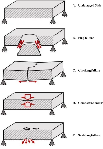
For concrete slabs loaded at the center and supported at the corners or sides (as illustrated in

Figure 2.5 A), existing research describes several qualitatively different failure modes [22]. The

most drastic type of failure, seen in cases of high-density impacts [11] or explosive detonations

[9], is that of plug formation. In this mode of failure the load is applied rapidly, and shear

stresses develop between the area under the footprint of the missile or charge and the free surface

of the slab. Cracks initiate near the top surface around the footprint, and propagate down at an

angle to the back face. The resulting truncated cone, called a plug, separates from the bulk of the

slab. This type of damage occurs immediately after impact, along the front of the primary

shockwave. It is illustrated in Figure 2.5 B.

For ballistic impacts at lower velocities, or for soft (deformable) projectiles, the contact time may

be somewhat longer, and the slab may begin to deform globally as well as locally. In this case

cracks will form in the tensile region of the slab, as shown in Figure 2.5 C. As the slab continues

to bend, the crack propagates upward to the front face. This is the primary mode of failure for

reinforced beams and walls impacted by a distributed load, and existing research [31] correlates

well to crack-based damage models of concrete [29]. Some thin slabs, however, may still

Figure 2.5 - Illustration of four common failure modes of concrete. Failure modes may occur independently, or together.

As the missile mass is decreased relative to the concrete slab, or the stiffness of the concrete

structure is increased by means of geometry or scale, impacts may not cause extensive damage.

Instead, the concrete may become compacted under the projectile or a pressure wave may cause

scabbing and spalling around the projectile, as show in Figure 2.5 D and E, respectively. These A. Undamaged Slab

B. Plug failure

C. Cracking failure

D. Compaction failure

two modes of failure do not threaten the structural integrity of the test specimen, but they are

important to consider for a multiple impact condition because of the high probability these sites

of local damage may become crack nucleation zones. In cases where concrete subjected to cyclic

loading, scabbing and spalling are indicators of zones of higher strain and softening.

It is not always clear which failure mode will be the dominant one for a given impact scenario.

Thinner slabs tend to fail by plug formation, while slabs that act as beams tend to crack. Any

concentrated load from a sharp projectile may also cause scabbing and compaction. For slabs

whose geometry does not fall into definite categories, failure modes occur concurrently, or

overlap. As a result, there is a justified reason for conservative design that avoids all failure

modes, though this approach may mask signs of weakening, and result in more extensive failure

when preventative maintenance is neglected [7]. Instead, structures that have more than one

defining characteristic and can experience multimodal failure may be analyzed with more than

one numerical model, to ascertain the dominant failure mode by means of agreement between

3.0

Methodology

3.1 Experimental Design

The purpose of the methodology section is to show the reasoning process behind the design of

the experiment and to explain in detail the methods used to study the progression of damage in a

multiple impact condition. In order to ensure their agreement, the computational model and

experimental test need to be developed concurrently, such that the geometry, timescale, damage

effects, and measurement methods are practical, in the physical and computational sense.

Based on a review of existing experimental methods, as given in section 2.3, a scale of 500 mm

to 1500 mm was proposed for the experimental tests. Due to safety concerns regarding the

shattering or rebound of the projectile, a lighter projectile was considered favorable. Finally, as

both the projectile and slab required a fine mesh during simulation, the lower bound of which

was determined by the aggregate size, the scale of the simulation needed to be such that the

element count rendered the computational problem tractable. These considerations may be called

the constraints of the research problem, and are summarized in Table 3.1. It can be seen from the

table that there are inherent tradeoffs in the design variables – a smaller simulation scale is

computationally efficient but detrimental to experimental error; a lower projectile speed

increases the anticipated number of tests until failure is achieved.

Table 3.1 – Constraints of the research problem. Dimensions are given as characteristic lengths.

Constraint Range Objective Justification

1. Slab dimensions 500 – 1500 mm Low = better Economy 2. Simulation scale 10 – 1000 k elements Low = better Economy

3. Projectile mass 1 – 10 kg Low = better Safety

Given enough studies where experiment and simulation are studied together using the same

testing methods and software, the solution to these constraints may be solved for by optimization

methods. However, the literature review showed low consistency of choice of experimental and

simulation methods among authors. The strategy for approaching the design of the four

experimental components (air cannon, slab, projectile, reinforcement bracket) and their

corresponding simulation counterparts was therefore as follows:

 First, a well-documented and relevant impact test was chosen from the literature, and

modeled in LS-DYNA. The resulting simulation could be studied to determine the

accuracy and efficiency of the LS-DYNA simulation environment. Various design

choices could be tried out and studied, such as the type of concrete material model,

timescale, mesh sizing, numerical convergence or instability, and formulation of

boundary conditions. This process is presented in Section 3.2.1, Preliminary work.

 Once the material model, mesh, geometry, and boundary conditions are decided on, a

sensitivity analysis of the specific model could be carried out with respect to initial

conditions such as impact velocity and to internal parameters such as erosion and failure

criteria. These results, documented in Section 3.2.1, extend the simulation behavior past

the reference experimental test, and give a thorough understanding of the model behavior

in trivial or extreme loading conditions. Additionally, these tests enable the tweaking of

any global solver settings, such as minimum time step or damping controls.

 Now that a reference experimental test is modeled by a simulation, an estimate of the

modified geometry and initial conditions is calculated. This effectively scales the design

variables to find a viable solution for defining the research problem. For instance, the

shown to be proportional to the projectile frontal area. From this information a ratio of

projectile size to slab size was selected, and scaled to minimize constraints 1, 3 and 5 in

Table 3.1. Slab thickness was then scaled down to allow significant damage, with the

corresponding adjustment to the measurement resolution.

 Finding a set of feasible problem constraints allows for the research problem to be

simulated. To conduct the experiment, however, the design of the constraining bracket

and air cannon is necessary. A separate design process is carried out for these assemblies

in the classical manner, using the physical dimensions of the slab and projectile, as well

as the initial velocity, as inputs. As long as the resulting design is not unreasonably

expensive or impractical, it may be selected without further revision.

In practice, this process was carried out over an iterative fashion over the course of some 8

months, and in conjunction with the acquisition of some of the measurement equipment. The

final values of the design variables are shown in the last column of Table 3.2. The first variables

to be decided on were the slab dimensions and thickness (not shown), and the last variables to be

tuned were projectile velocity and mass. The following sections will describe the specific

reasoning behind these values, and cover the methods of acquiring and processing data.

Table 3.2. Reference and final values of the design variables.

Constraint Range Reference Value Final Value

1. Slab dimensions 500 – 1500 mm 1200 mm 600 mm

2. Simulation scale 10 – 1000 k elements 5 k elements 48 k elements

3. Projectile mass 1 – 10 kg 6.8 kg 2.0 kg

3.2 Simulation Methodology

3.2.1 Preliminary work.

The National Storm Shelter Association (NSSA) Frontal Impact Test was selected as the

reference test for this research paper, due to its well-documented setup and its use in providing

certification for storm protection [2]. The test specifies that a 4x4 foot section of protective

material impacted by a 15 lb wood stud is rated for a type of severe storm if it can prevent the

perforation of the projectile accelerated to the corresponding rated speed. In the case of an EF-5

tornado, for example, the rated wind speed is in excess of 300 mph, and the rated projectile speed

is 100 mph for horizontal surfaces [3]. The successful simulation of the test was the first

significant milestone in the characterization of concrete impact dynamics. See Figure 3.1 for a

visual of the simulation.

The figure shows a pressure shock wave propagating through the wood stud at the time of 6.82

ms, after the wood rebounded. A zone of residual strain and compaction can be seen in a

cross-section of the concrete, depicted in Figure 3.2. The residual plastic strain extends several

millimeters into the surface, and has a high value (0.25), indicative of softer, compacted concrete

or masonry. No damage extends to the back of the slab. This is consistent with the type of

compaction that may be seen in low-strength residential-grade concretes, although this type of

damage would be unacceptable in protective structures, where strain should not exceed 0.01.

Figure 3.2. Effective plastic strain remaining after impact.

Besides visual results obtained from the simulation, the nodal displacements and accelerations of

the concrete slab were tracked at the centers of the front and back face. These provided helpful

information on the type of acceleration data that may be collected by a center-mounted

accelerometer in a physical test, and the type of displacements a slab may experience. Figure 3.3

milliseconds. These results gave insight into the duration of impact and the time step resolution

needed to accurately track variables. The figure also shows how the plastic deformation of the

concrete material in the front causes a dilation of the vibrational response frequency.

Figure 3.3. Acceleration nodal histories for the preliminary impact simulation.

A damage variable in the RHT concrete model allowed the assessment of compound damage,

and the depth and area of the damage zone were found to be roughly half and twice the missile

diameter, respectively [24]. In the case of a compaction failure, the damage was confined to the

zone of plastic strain, and the damage visualization is essentially the same as that in Figure 3.2.

The initial simulation was optimized to run in a matter of minutes, to allow for easy

troubleshooting. Mesh elements not in the immediate zone of impact were left very coarse,

leaving the majority of the elements near the contact region. The model consisted of roughly

6200 elements, with element sizes ranging from 150 mm to 10 mm. Following these promising

results, additional simulations of different sizes and qualities of mesh were performed. The

results showed fair agreement with the initial effort. A

B

A

Further useful insights were obtained from varying material parameters, as well as environmental

variables. For instance, temperature and moisture effects were considered in the design of impact

tests. The differences in nodal displacements for each scenario are summarized in Figure 3.4.

The penetration depth difference was observable, but not significant.

Figure 3.4. Penetration depth at various simulated environmental conditions. Legend shows % MC and deg C.

Finally, the impact speed was varied over a wide range to obtain a speed-deflection characteristic

curve. The simulation data of the CSCM and RHT concrete models was compared to the

predictions given by the NDRC and Kar formulas, and were found to lie between them. Figure

3.5 shows the data obtained.

-6 -5 -4 -3 -2 -1 0

0 2 4 6 8 10 12

Pen

e

tr

ation

D

e

p

th

(

m

m

)

Time (ms)

Penetration Variation due to Temp. and Moisture

0% 0C

20% 30C

Figure 3.5. Velocity-dependent penetration predictions for soft missiles.

No tensile or plug failure occurred during the frontal impact test. To understand the difference in

failure progression between concrete models, an unreinforced corner impact was modeled, as

seen in Figure 3.6. The RHT and CSCM materials were compared, and erosion criteria were

varied to determine the dependency of the dynamic behavior on the failure mode. Individual

elements were found to display unrealistic strains after surpassing critical damage, however, the

simulation displayed greater numerical stability and showed a comparable area of erosion with

the RHT damage variable.

0.1 0.5 5.0 50.0

20 40 60 80 100 120 140

M

ax.

Pe

n

e

tr

ation

(

m

m

)

Impact Speed (m/s)

Penetration Predictions for Soft Impacts

CSCM

RHT

NDRC

Figure 3.6. Corner impact test visualizations. RHT is on the left and CSCM is on the right.

Following the completion of these preliminary tests, the design variables for the final tests were

finalized. The materials for the slab, projectile, and reinforcement were selected based on ease of

use, numerical stability and intent of application.

3.2.2 Geometry

In order to accurately model the impact of a projectile into an RC slab, full-scale part geometries

were created for the slab assembly (concrete and rebar) and the projectile assembly (wood stud

and metal end-caps). The concrete was modeled as a 24x24x4 inch slab, and the rebar was

modeled as 0.125 inch diameter wire spaced 6 inches apart to create a lattice. The rebar was

positioned 1.0 inch from the back face of the slab. The solid models of the projectile, target slab

and rebar were generated in Solidworks and exported to ANSYS. An illustration of the

simulation model may be found in Figure 3.7. The model reflects the dimensions specified in the

Figure 3.7. Illustration of the simulation model, showing the slab and composite projectile, as well as the element mesh.

3.2.3 Element and mesh

The projectile and target are discretized using default ANSYS 8-node hexahedral elements,

which are then converted to a single point 8-node hexahedral element in LS-PrePost. These

elements are simple and efficient, but possess zero-energy mode of deformation, where element

nodes may move without the element experiencing average strain. A 3-node line element is used

to mesh the rebar. Concrete element size was constrained to 10 mm to approximate the aggregate

diameter. The projectile mesh was sized at 8 mm, to be comparable in scale to the slab mesh.

The rebar, which was modeled as one-dimensional line elements, takes on a 20 mm element

3.2.4 Material models

The materials used in the simulation are concrete, steel, and wood. Each material was assigned a

model based on its anticipated behavior experimentally. Table 3.3 below summarized the

material selection and full input parameters can be found in the LS-DYNA input deck in

Appendix B. Default material properties, as determined by the developers of the material model,

were selected unless otherwise noted in the table.

Table 3.3. Summary of material model selections.

Material Role Anticipated behavior Material model Controlled properties

Wood Projectile Nonlinear, Anisotropic MAT_143 (USDOT) Density

Concrete Target slab Nonlinear, Isotropic MAT_272 (RHT) Compressive strength Steel Caps, Rebar Linear Elastic, Isotropic MAT_003 (Elastic) Density, Elastic mod.

3.2.5 Contact formulation

All projectile and slab element contacts were controlled by an automatic single contact

algorithm, which and allows for penalty-based contact between any two penetrating elements. In

this way, contact forces are applied from slab to projectile, but not between projectiles, so that a

rebounding projectile would not interact with an incoming one in the multiple impact simulation.

A special constraint formulation, “Constrained Lagrange in Solid” was used to relate the

displacement and velocity of the nodes in the rebar to the nodes in the solid concrete element

surrounding it. In this manner, the concrete elements containing the rebar will have the strength

of steel as well as the concrete, while maintaining failure modes of both materials independently.

3.2.6 Timescale

The simulation time step is determined by the time interval a shockwave takes to travel through

the smallest element. In this case, the steel components determine the size of the timestep, and

LS-DYNA automatically makes an initial prediction from the element geometries. During the

simulations run with the geometry described above had a time step on the order of 1E-6s, giving

a resolution of 1000 steps per millisecond. The system state is written to a database on a larger,

user-specified timescale of 0.1 milliseconds. In addition, every 5000 time steps, runtime statistics

are calculated, showing average computational time per cycle, ranging from 100 ms to a few

seconds. In this manner, simulation stability can be tracked.The control parameters input into

the simulation can be found in Appendix B.

3.2.7 Post-processing procedure

After the simulation has completed, a standard procedure is followed to verify accuracy and to

obtain standardized, comparable results. Because of the explicit solver used, a review of part

energies over the time history of the simulation is important to verify energy conservation and

hence simulation accuracy. Additionally, tracking the hourglass energy for all reduced

integration point elements ensures that deformations are due to physical strains and not

zero-energy modes of the elements. Table 3.4 below summarizes the sequence of actions to process

simulation results.

Table 3.4. Summary of post-processing steps.

P01 Run simulation and write files to LS-DYNA database.

P02 Load simulation files into LS-PREPOST.

P03 Check simulation stability over the timescale.

P04 Track the kinetic energy of the slab part to ensure proper energy dissipation.

P05 Track the nodal acceleration in the impact region to obtain the concrete's modal response.

P06 Identify the stresses and strains in the impact region.

P07 Identify the extent of damage using the damage variable.

P08 Export the deformed state of the elements for further simulation work.

3.3 Experimental Methodology

The experimental setup was designed primarily with the purpose of safety in mind. The air

cannon, power equipment, user controls and trajectory alignment were positioned away from the

impact to minimize health hazards. The slab was constrained in the reinforcing bracket and

covered on the sides by a protective enclosure consisting of plywood and cinderblock. The

enclosure prevented debris generated on impact from flying out of the designated impact zone.

Figure 3.8. Schematic of test setup and equipment. The user activated a high-flow-rate valve between the air tank and barrel. Which triggered data collection from both accelerometers.

3.3.1 Projectile

The projectile consisted of a rectangular beam of spruce wood with two metal end caps, and was

wrapped in duct tape to prevent splintering on impact. Projectile dimensions were 30” long and

1.5x3.5” in cross section, as detailed in Appendix A. Projectile masses were kept consistent to

1950g +/- 50g. Ten interchangeable projectiles were fabricated to allow for replacement mid-test.

Projectiles were found to crack and buckle after a few impacts.

3.3.2 Concrete slab pour

The concrete slabs were created by mixing and pouring Quikrete 5000 industrial concrete mix

according to manufacturer recommended instructions. One batch per slab was prepared using an

0.125 inch steel wire. Two test samples per slab were poured into 2x2x2 inch ASTM molds at

the time of the pour, and allowed to cure in lab conditions alongside the concrete slab.

Compressive tests were carried out on concrete samples after 4 weeks of curing. The test

procedure is given by ASTM C109 [1]. The compressive strength was found to be 32.5 MPa,

with a standard deviation of 1.6 MPa.

3.3.3 – Air cannon.

A dedicated air cannon was fabricated for testing, following the design of pneumatic projectile

launch devices described in ASTM E1886 [2]. Refer to Appendix A for design dimensions. The

air cannon was expected to operate at pressures as high as 690 kPa, and accelerate the projectile

to speeds of 40 m/s. In practice, a more conservative speed of 20 m/s proved to be sufficient for

creating a damaging impact.

3.3.4 - System Calibration.

Preliminary analysis and tests showed that a repeatable impact location was important for

obtaining consistent vibrational response results. The slab was positioned 1.0 m away from the

air cannon barrel to minimize free-flight time. The air cannon orientation was adjusted optically

at the beginning of the test so that the projected impact location was within 5% of the geometric

center of the slab (25 mm deviation). Subsequent projectile firings resulted in a high repeatability

of within 2% of the initial impact location. Projectile speed varied due to friction and pressure

release conditions, and was repeatable to within 10% of the mean value.

3.3.5 – Data acquisition.

Two accelerometers from PCB Piezotronics (Model 353B03) were selected to mount on the air

cannon and the back face of the slab. The accelerometers collected data up to 300 g and 7000 Hz.

were triggered to begin data acquisition by the initial acceleration of the air cannon valve. Data

for projectile impact was synchronously recorded for 3000 ms after the trigger was tr