Indirect RBFN Method with Thin Plate Splines for Numerical Solution of
Differential Equations
N. Mai-Duy, T. Tran-Cong1
Abstract: This paper reports a mesh-free Indirect Ra-dial Basis Function Network method (IRBFN) using Thin Plate Splines (TPSs) for numerical solution of Dif-ferential Equations (DEs) in rectangular and curvilinear coordinates. The adjustable parameters required by the method are the number of centres, their positions and possibly the order of the TPS. The first and second order TPSs which are widely applied in numerical schemes for numerical solution of DEs are employed in this study. The advantage of the TPS over the multiquadric basis function is that the former, with a given order, does not contain the adjustable shape parameter (i.e. the RBF’s width) and hence TPS-based RBFN methods require less parametric study. The direct TPS-RBFN method is also considered in some cases for the purpose of comparison with the indirect TPS-RBFN method. The TPS-IRBFN method is verified successfully with a series of problems including linear elliptic PDEs, nonlinear elliptic PDEs, parabolic PDEs and Navier-Stokes equations in rectan-gular and curvilinear coordinates. Numerical results ob-tained show that the method achieves the norm of the rel-ative error of the solution of O(10−6)for the case of 1D second order DEs using a density of 51, of O(10−7)for
the case of 2D elliptic PDEs using a density of 20×20 and a Reynolds number Re=200 for the case of Jeffery-Hamel flow with a density of 43×12.
keyword: mesh-free indirect RBFN method, thin plate splines, rectangular coordinates, curvilinear coordi-nates, Jeffery-Hamel flow, numerical solution, differen-tial equation.
1Corresponding author: Telephone +61 7 46312539, Fax +61 7 46 312526, E-mail [email protected]
Faculty of Engineering and Surveying,
University of Southern Queensland, Toowoomba, QLD 4350, Aus-tralia
1 Introduction
parameter (i.e. the RBF’s width). A method for deter-mining the optimal value of the shape parameter is yet to be found. There is increasing interest in another RBF in numerical schemes for DEs [Zerroukat, Power and Chen (1998); Zerroukat, Djidjeli and Charafi (2000)], namely the Thin Plate Splines (TPS). The theoretical foundations for this basis function were laid by Duchon (1977). It is interesting that, even with less adjustable parameters, the TPS-based RBFN methods can achieve an accuracy sim-ilar to that of the MQ-based method [Zerroukat, Djidjeli and Charafi (2000)]. In this paper, the Indirect RBFN method using TPSs is developed and verified in rectangu-lar and curvilinear coordinates. It should be emphasised here that in this work the employment of numerical inte-gration schemes is introduced in order to deal with the so-lution of high order DEs and problems in curvilinear co-ordinates. The paper is organised as follows. The second section presents the numerical formulation of the TPS-IRBFN method for solving DEs in rectangular coordi-nates and then some test problems governed by linear el-liptic PDEs, nonlinear elel-liptic PDEs and parabolic PDEs are simulated to verify the present method. The third sec-tion is to present the implementasec-tion of the TPS-IRBFN method in curvilinear coordinates which is verified by the solution of linear Poisson’s equation and Navier-Stokes equations. The last section gives some concluding re-marks.
2 TPS-IRBFN methods in rectangular coordinates
2.1 Numerical formulation
The basic derivation of the IRBFN method is given else-where [Mai-Duy and Tran-Cong (2001a,b,2002)] and further developed here with the use of the Thin Plate Spline given by
g(i)=R2qlog(R), (1)
where q is the order of the TPS and R is the Euclidean dis-tance between the ith centre ccc(i)and the collocation point
xxx, i.e. R=ccc(i)−xxx
2, in which ccc,xxx∈ℜdand d is any
pos-itive integer [Schaback (1995); Gutmann (2001); Forn-berg, Driscoll, Wright and Charles (2002)]. However, in 2D, TPSs are rigorously justified with extensive theoret-ical accuracy results and a variational theory as reported by Fornberg, Driscoll, Wright and Charles (2002) who have applied the TPS RBF (1) approximation in a 1D problem. Thus the TPS RBF (1) is applicable in one, two
and three dimensions. In the present method the highest order derivatives are expressed in terms of TPS-RBFNs first, followed by successive symbolic integrations to ob-tain closed form expressions for lower order derivatives and finally the function(s) itself. The general procedure is briefly recaptured as follows. Consider the variableψ in the governing equation, the functionψand its deriva-tives with respect to xj can be decomposed in terms of
basis functions as follows
ψ,j j(xxx) = m
∑
i=1w(i)g(i)(xxx), (2)
ψ,j(xxx) =
ψ,j j(xxx)dxj= m
∑
i=1w(i)
g(i)(xxx)dxj, (3)
ψj(xxx) =
ψ,j(xxx)dxj
=
∑
mi=1
w(i)
g(i)(xxx)dxj
dxj. (4)
where m is the number of centres,g(i)m1 the set of radial basis functions and w(i)m1 the set of RBFN weights. The closed form representations in terms of basis func-tions thus obtained are then substituted into the govern-ing equations and boundary conditions to “discretise” the system via the mechanism of point collocation at xxx(i)n1
where n is the number of collocation points [Mai-Duy and Tran-Cong (2001a)]. This process reduces com-plex systems of differential equations to systems of alge-braic equations with the unknown vector being the set of RBFN weights, which can be solved directly by standard numerical algorithms. For the purpose of illustration, let us consider the 2D Poisson’s equation over the domainΩ
∇2u=p(xxx), xxx∈Ω, (5)
where∇2is the Laplacian operator, xxx is the spatial posi-tion, p is a known function of xxx and u is the unknown function of xxx to be found. Equation (5) is subject to Dirichlet and/or Neumann boundary conditions over the boundaryΓ
u=p1(xxx), xxx∈Γ1, (6)
nnn·∇u=p2(xxx), xxx∈Γ2, (7)
such asΓ1∪Γ2=ΓandΓ1∩Γ2=/0; p1and p2are known
functions of xxx.
The information provided by the given DEs and the asso-ciated boundary conditions are taken into account in de-signing the networks through the following Sum Squared Error (SSE)
SSE=
∑
xxx(i)∈Ω
(u,11(xxx(i)) +u,22(xxx(i)))−p(xxx(i))
2
+
∑
xxx(i)∈Ω
u1(xxx(i))−u2(xxx(i))
2
+
∑
xxx(i)∈Γ1
u1(xxx(i))−p1(xxx(i))
2
+
∑
xxx(i)∈Γ2
(n1u,1(xxx(i)) +n2u,2(xxx(i)))−p2(xxx(i))
2
, (8)
where the term u1(xxx(i))is symbolically obtained via u,11
and u2(xxx(i))via u,22 in the manner of (2)-(4) above. By
substituting the representations for u and its derivatives (2)-(4) into (8), the unknowns in the governing equations are now RBFN weights that are to be found by the pro-cess of minimisation. Note that in the present context of solving DEs, the “data” points are more general colloca-tion points instead of just actual given numerical values of the function to be approximated or interpolated. Thus at a data (collocation) point either the DEs (in the case of internal points) or the DEs and the boundary conditions (in the case of boundary points) are forced to satisfy. The
SSE above can be rewritten in the short form as
minAwww−yyy2, (9)
where A is regarded as the design matrix, yyy is a known vector and www the solution to be found. Normally, if the
two sets of centres and collocation points are identical, A is non-square and of dimension N×M with M>N.
Note that in general A can be determined, overdeter-mined or underdeteroverdeter-mined depending on the number of centres and the number of collocation points employed. The number of columns of A, i.e. M, is decided by the number of centres m and the number of constants of inte-gration while the number of rows N depends on the num-ber of collocation points n.
2.2 Linear least squares problem
The goal here is to find the solution www of the Linear
Least Squares (LLS) problem (9). The problem has a unique solution or infinitely many solutions depending on the characteristic of a matrix A∈ RN×M. In the
case of N ≥M and A has full rank then Awww=yyy has
a unique solution. Otherwise, if A is rank deficient, there exist infinitely many solutions and the minimum norm L2 solution minx2 is usually the required
solu-tion to the LLS problem. In the case of N<M, there
exist infinitely many solutions to the underdetermined linear system Awww =yyy, but the LLS problem still has
a unique minimum norm L2 solution where the
combi-nation of “irrelevant” basis functions if existed will be driven down to a small value rather than pushed up to delicately cancelling infinities. The Singular Value De-composition (SVD) of a matrix A is a matrix decomposi-tion of great theoretical and practical importance for the treatment of least squares problem and becomes a main tool in numerous application areas [Bjorck (1996)]. SVD produces a solution that is the best approximation in the least-squares sense for an overdetermined system, or a solution whose values are smallest in the least-squares sense for an underdetermined system [Press, Flannery, Teukolsky and Vetterling (1988)] and will be employed in the present IRBFN procedure. Let p be min(M,N), the singular value decomposition of A can be written in the form
A=UΣΣΣVT= p
∑
i=1uiσivTi, (10)
where U = (u1,...,up) and V= (v1,...,vp) are
or-thogonal matrices and ΣΣΣ =diag(σ1,...,σp) has
non-negative diagonal elements appearing in non-increasing order such that
σ1≥σ2≥...≥σp. (11)
The condition number of A is defined as the ratio be-tween the largest and smallest singular valuesσ1/σp. If
2.3 Numerical examples
A measure of the relative error of the solution or the norm of the error of the solution, Ne, is defined as
Ne=
∑n
i=1(ue(xxx(i))−u(xxx(i)))2
∑n
i=1ue(xxx(i))2
, (12)
where u(xxx(i))and ue(xxx(i))are the calculated and exact
so-lution at the point i respectively and n is the number of collocation points.
2.3.1 Example 1 - 1D linear Poisson’s equation
Consider the following 1D second order equation
∇2u=−16π2sin(4πx) (13)
defined on 0≤x≤1 with u=2 at x=0 and x=1. The exact solution can be verified to be
ue(x) =2+sin(4πx). (14)
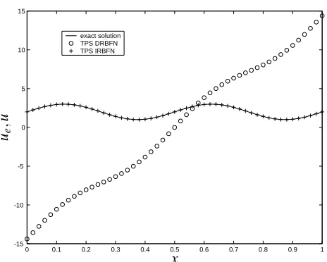
A set of 51 points distributed uniformly on the computa-tional domain 0≤x≤1 is chosen to be the set of cen-tres and also the set of collocation points. As mentioned above, the interior collocation points are forced to sat-isfy the DEs while the boundary collocation points are to satisfy both the DEs and the boundary conditions. In or-der to assess the performance of the present TPS-IRBFN method, the Direct RBFN (DRBFN) method [Mai-Duy and Tran-Cong (2001a)], but with the TPS replacing the MQ-RBFs is also employed. Results are displayed in Figure 1 with the error norms being 4.110e0 and 1.805e−6 for TPS-DRBFN and TPS-IRBFN method, respectively, where the second order TPS are used in both cases. The TPS-IRBFN method yields a very high ac-curacy while the opposite is true for TPS-DRBFN ap-proach. Another scheme for TPS-DRBFN is employed where the boundary collocation points are used only for the satisfaction of the boundary conditions, resulting in a determined linear system of equations. In this case, the TPS-DRBFN result is improved with the error norm be-ing 1.245e−3 which is still much greater than that asso-ciated with the TPS-IRBFN method (Ne=1.805e−6).
In the case of the first order TPS, which is C1 continu-ous, only the IRBFN method can be established and the error norm achieved is 5.051e−5. All of the error norms are presented in Table 1 showing that the TPS-IRBFN method, especially with the second order TPS, yields much better results than the TPS-DRBFN approach.
0 0.1 0.2 0.3 0.4 0.5 0.6 0.7 0.8 0.9 1
-15 -10 -5 0 5 10 15
exact solution TPS DRBFN TPS IRBFN
x
ue
,
[image:4.612.320.552.128.314.2]u
Figure 1 : Solution of ∇2u=−16π2sin(πx): plots of the exact solution and the approximate solutions obtained from the DRBFN (non-square matrix) and IRBFN pro-cedures with second order TPS. The centre density is 51 and uniformly distributed. The results show that the DRBFN method does not achieve an accuracy compara-ble with the IRBFN method.
Table 1 : 1D linear Poisson’s equation: Comparison of the norm of the relative error of the solution Neobtained
by the usual TPS-DRBFN and the present TPS-IRBFN methods. Note that the DRBFN method using the first order TPS is not possible for the second order DEs be-cause the basis function is only C1continuous.
Ne q=1 q=2
DRBFN − 4.110
(overdetermined system)
DRBFN − 1.245e−3
(determined system)
[image:4.612.317.559.599.684.2]2.3.2 Example 2 - 2D linear Poisson’s equation
The problem here is to determine a function u(x1,x2)
sat-isfying the following PDE
∇2u=sin(πx
1)sin(πx2) (15)
defined on the rectangle 0≤x1≤1, 0≤x2≤1 subject to
the Dirichlet condition u=0 along the whole boundary of the domain. The exact solution is given by
ue(x1,x2) =−
1
2π2sin(πx1)sin(πx2). (16)
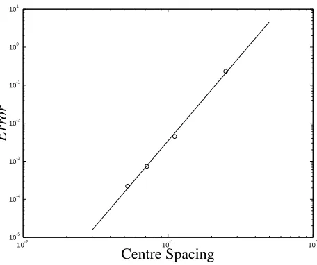
[image:5.612.323.551.95.286.2]Four centre densities of 5×5, 10×10, 15×15 and 20×20 are employed to verify the present method. Re-sults for the second order TPS-DRBFN are shown in Table 2 from which it can be seen that the results cor-responding to the determined system are more accurate than those corresponding to the overdetermined system. Tables 2 and 3 show that the TPS-IRBFN method, espe-cially with the second order TPS, yields better accuracy than the TPS-DRBFN approach. The rate of convergence of the TPS-IRBFN method can be estimated via a plot of the error norm versus the density space. A set of 41 test points are employed to compute the error norms for four different centre densities. The solution converges appar-ently as h4.479where h is the centre spacing (Figure 2).
2.3.3 Example 3 - 2D nonlinear Poisson’s equation
Thermal conduction with nonlinear heat generation is considered in this example. The temperature distributing in a homogeneous solid can be described by the follow-ing PDE
∇2T = f(T). (17)
In the present work, the heat generation is given by an exponential function of temperature f(T) =−0.5 exp(T)
which is the same as in Zheng and Phan-Thien (1992). A square domain with dimensions [0,1]×[0,1]is chosen for analysis. The boundary condition T =1 is prescribed along two sides x1=0 and x2=0 and the adiabatical
condition ∂T/∂n=0 along the other two sides x1=1
and x2=1 where n is the coordinate direction of the unit
outward normal vector at the boundary. In order to deal with the nonlinear term f(T), the iterative procedure is employed according to the following steps
1. Render the nonlinear term linear by using the tem-perature field obtained from the previous iteration.
10-2 10-1 100
10-5
10-4
10-3
10-2
10-1
100
101
Centre Spacing
Er
ro
r
[image:5.612.339.537.456.555.2]Figure 2 : Solution of∇2u=−16π2sin(πx): the rate of convergence with centre density refinement. The errors here are defined as norms of the relative error between the exact solution and the computed solutions for the cases of density 5×5, 10×10, 15×15 and 20×20 based on the same set of 41×41 test points. The solution converges apparently as h4.479where h is the centre spacing.
Table 2 : 2D linear Poisson’s equation: Error norms Nes
of the solution obtained by the DRBFN method with sec-ond order TPS.
Density Ne Ne
(overdetermined (determined system) system) 5×5 2.819 3.382e−2 10×10 2.529 5.413e−3 15×15 2.297 1.787e−3 20×20 2.062 7.770e−4
Table 3 : 2D linear Poisson’s equation: Error norms Nes
of the solution obtained by the IRBFN method with first and second order TPSs.
Density Ne Ne
1.05
1.15
1.25 1.35
1.45 1.55
1.6
1.05 1.15
1.25
1.35
1.45 1.55
1.6
1.05 1.15
1.25
1.35
1.45 1.55
1.6
1.05 1.15
1.25
1.35 1.45
1.55 1.6
9×9 13×13
[image:6.612.106.508.80.424.2]17×17 21×21
Figure 4 : Solution of∇2T=−0.5 exp(T): plots of the distribution of temperature obtained by the IRBFN method with second order TPS corresponding to four different centre densities.
1 2 3 4 5 6 7 8 9 10 11
10-5
10-4
10-3
10-2
10-1
100
9× 9
13× 13
17× 17
21× 21
Number of iterations
CM
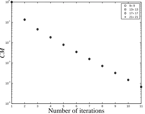
Figure 3 : Solution of∇2T=−0.5 exp(T): Convergence
measure based on the norm of the difference of the tem-perature field between two successive iterations.
Note that for the first iteration the initial tempera-ture field needs to be guessed (in the present work it is simply initialized to zero);
2. Apply the TPS-IRBFN procedure to obtain the new estimate of the temperature field;
3. Compute the convergence measure CM defined as
CM=
∑n
i=1(Tk(xxx(i))−Tk−1(xxx(i)))2
∑n
i=1(Tk(xxx(i)))2
,
where k denotes the current iteration and n is the number of collocation points;
4. Check for convergence. If CM<tol where tol is a
set tolerance, the solution procedure is terminated. Otherwise, repeat from the step 1.
[image:6.612.64.298.491.676.2]cases converge after 11 iterations (Figure 3) with the re-sulting temperature fields displayed in Figure 4. It can be seen that there is a good agreement between the tempera-ture fields obtained from four centre densities employed. Another way to estimate the convergence of the iterative procedure is to use the norm of temperature [Zheng and Phan-Thien (1992)] which is defined as
NT=
∑n
i=1Ti2
[image:7.612.322.553.122.308.2]n .
Figure 5 shows the norm of temperature NT versus the
number of iterations. The change of NT is very small
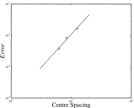
at the iteration number 11 where the solution can be re-garded as convergent. In order to estimate the rate of con-vergence with mesh refinement, the solution correspond-ing to the finest centre density 21×21 is taken to be “ex-act”. Results for lower centre densities are mapped onto the grid points 21×21 by IRBFN interpolation, from which the norm of the error relative to the “exact” so-lution is calculated. A plot of these errors is shown in Figure 6 as a function of the grid spacing h. The solution converges apparently as h2.1041.
2.3.4 Example 4 - Parabolic PDE
The problem under consideration here is governed by
1
K
∂u(xxx,t)
∂t +g(xxx,t) =∇
2u(xxx,t), xxx∈Ω, t>0, (18)
where Ωis the domain of analysis[0,1]×[0,1], K is a positive constant and g is the forcing function. In the present work, K =1 and
g(xxx,t) =sin(x1)sin(x2)(2 sin(t)cos(t))
as in Ingber and Phan-Thien (1992). The initial and boundary conditions yield the following solution
u(xxx,t) =sin(x1)sin(x2)sin(t).
A method of discretisation in space-time is employed whereby the spatial variables are discretised using the TPS-IRBFN procedure and time is discretised using the finite difference method. Only first order finite differ-ence approximation for the time derivative is considered in this work
∂u(n)
∂t ≈
u(n)−u(n−1)
∆t , (19)
1 2 3 4 5 6 7 8 9 10 11
1.05 1.1 1.15 1.2 1.25 1.3 1.35
9× 9
13× 13
17× 17
21× 21
Number of iterations
NT
Figure 5 : Solution of∇2T=−0.5 exp(T): Convergence
measure based on the norm of the temperature field NT.
10-2
10-1
100
10-5
10-4
10-3
10-2
Centre Spacing
Er
ro
r
[image:7.612.320.553.383.572.2]where∆t is the time step and u(n)=u(xxx,t(n)=n∆t).
Sub-stitution of (19) into (18) yields
∇2u
(n)−κ2u(n)=g(n)−κ2u(n−1), (20)
where κ2=1/(K∆t). With u(n−1) already known from
the previous step t(n−1), the PDE with the unknown u(n) can be solved by the TPS-IRBFN method. Two centre densities 6×6 and 11×11 are employed. Results at the interior point x1 =0.8 and x2 =0.8 for the coarse and
fine densities using a time step of 0.25 are displayed in Table 4. The results of the two cases are close to the ex-act solution. The results for the fine density is slightly better than those for the coarse density as expected. Re-sults at the interior point x1=0.3 and x2=0.7 generated
[image:8.612.342.534.157.406.2]using the fine mesh and for two different time steps are displayed in Table 5. The results using the smaller time steps are seen to be more accurate. Figure 7 shows a good agreement between the exact and approximate solutions at time t=8.
Table 4 : 2D parabolic PDE: Results by the IRBFN method with second order TPS for the interior point
x1=0.8 and x2=0.8.
Time TPS-IRBFN,∆t=0.25 Analytic 6×6 11×11
0.25 0.127073 0.127075 0.127314 0.50 0.246100 0.246103 0.246712 0.75 0.349809 0.349813 0.350771 1.00 0.431766 0.431772 0.433020 1.25 0.486877 0.486884 0.488347 1.50 0.511717 0.511725 0.513310 1.75 0.504741 0.504748 0.506358 2.00 0.466382 0.466389 0.467924 2.25 0.399026 0.399032 0.400396 2.50 0.306861 0.306865 0.307973 2.75 0.195616 0.195619 0.196402 3.00 0.072209 0.072210 0.072620 3.25 -0.055687 -0.055688 -0.055677 3.50 -0.180122 -0.180124 -0.180512 3.75 -0.293357 -0.293361 -0.294125 4.00 -0.388353 -0.388358 -0.389450
Table 5 : 2D parabolic PDE: Results by the IRBFN method with second order TPS for the interior point
x1=0.3 and x2=0.7.
Time TPS-IRBFN, 11×11 Analytic
∆t=0.5 ∆t=0.25
0.50 0.0904 0.0907 0.0912 1.00 0.1582 0.1591 0.1601 1.50 0.1872 0.1885 0.1899 2.00 0.1703 0.1717 0.1731 2.50 0.1118 0.1129 0.1139 3.00 0.0258 0.0264 0.0268 3.50 -0.0663 -0.0664 -0.0667 4.00 -0.1424 -0.1431 -0.1440 4.50 -0.1835 -0.1847 -0.1861 5.00 -0.1797 -0.1811 -0.1825 5.50 -0.1319 -0.1332 -0.1343 6.00 -0.0518 -0.0526 -0.0531 6.50 0.0409 0.0408 0.0409 7.00 0.1237 0.1243 0.1250 7.50 0.1762 0.1773 0.1785 8.00 0.1855 0.1869 0.1883
0 0.25
0.5 0.75 1
0 0.25 0.5 0.75 1 0 0.2 0.4 0.6 0.8
0 0.25
0.5 0.75 1
0 0.25 0.5 0.75 1 0 0.2 0.4 0.6 0.8
x1
x2 ue
Exact Solution
x1
x2
u
[image:8.612.79.285.447.696.2]Approximate Solution
Figure 7 : Solution of Parabolic PDE by the IRBFN with second order TPS using a centre density of 11×11: plots of exact solution and approximate solution at the time
[image:8.612.320.552.464.651.2]2.3.5 Example 5 - 3D linear Poisson’s equation
The problem here is to determine a function u(x1,x2,x3)
satisfying the following PDE
∇2u=−
∂ u
∂x1 +
∂u
∂x2+
∂u
∂x3
(21)
defined on the cube 0≤x1≤1, 0≤x2≤1, 0≤x3≤
1 subject to the Dirichlet condition u =exp(−x1) +
exp(−x2) +exp(−x3)on the whole boundary of the
do-main. The exact solution is given by
ue(x1,x2,x3) =exp(−x1) +exp(−x2) +exp(−x3). (22)
Three centre densities of 3×3×3, 5×5×5 and 7×7×7 are employed to verify the present method. Results for the first order TPS-DRBFN are shown in Table 6 from which it can be seen that the applicability of the TPS
[image:9.612.316.563.443.563.2]R2qlog(R)in 3D is also verified and the method exhibits excellent mesh-convergence.
Table 6 : 3D linear Poisson’s equation: Error norms Nes
of the solution obtained by the IRBFN method with first order TPS.
Density Ne
3×3×3 1.301e−4 5×5×5 5.525e−6 7×7×7 9.405e−7
3 TPS-IRBFN method in curvilinear coordinates
3.1 Numerical formulation
For problems on polar or cylindrical domains, it may be more efficient to use curvilinear coordinates and the aim here is to demonstrate the working of the present method in such situations. For 2D problems, the first step is to transform the rectangular coordinates into the convenient polar or cylindrical coordinates. Consider the thin plate splines
g(i)(x1,x2) =R2qlog(R),
where q is the order of the TPS and R is the Euclidean distance between the ith centre ccc(i) and the collocation point xxx, i.e. R=ccc(i)−xxx
2. Applying the polar
coordi-nate transformation, x1=r cos(θ), x2=r sin(θ), where
r= x2
1+x22andθ=arctan(x2/x1), then TPS becomes
g(i)(r,θ) =
(r cos(θ)−r(i)cos(θ(i))
2
+
r sin(θ)−r(i)sin(θ(i)) 2q
log
(r cos(θ)−r(i)cos(θ(i))
2
+
r sin(θ)−r(i)sin(θ(i))
21/2
(23)
Similarly, this transformation can also be used to obtain the new forms of the governing equations and the asso-ciated boundary conditions in polar coordinates. For ex-ample, in polar coordinates, the Poisson’s equation (5) now takes the form
∂2u
∂r2 +
1
r
∂u
∂r +
1
r2 ∂2u
∂θ2 =p(r,θ). (24)
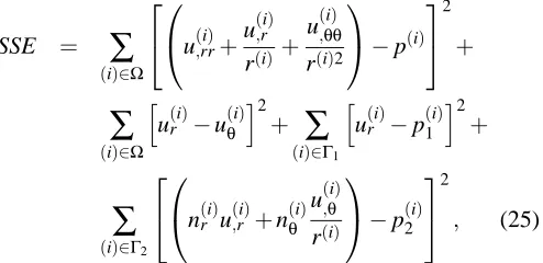
The corresponding SSE which is employed in designing the networks for obtaining numerical solution of (5), (6) and (7) can be written in polar coordinates as follows
SSE =
∑
(i)∈Ω
u(,rri)+
u(,ri) r(i)+
u(,θθi) r(i)2
−p(i)
2
+
∑
(i)∈Ω
u(ri)−u(θi) 2
+
∑
(i)∈Γ1
u(ri)−p(1i) 2
+
∑
(i)∈Γ2
n(ri)u(,ri)+n(θi) u(,θi) r(i)
−p(2i)
2
, (25)
where the term uris obtained via u,rrand uθvia u,θθ.
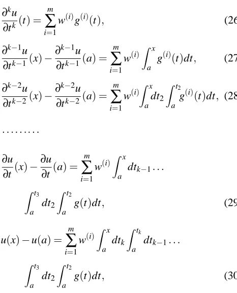
consideration, then the function u and its derivatives are expressed in terms of basis functions as
∂ku
∂tk(t) = m
∑
i=1w(i)g(i)(t), (26)
∂k−1u ∂tk−1(x)−
∂k−1u ∂tk−1(a) =
m
∑
i=1w(i)
x
a
g(i)(t)dt, (27)
∂k−2u ∂tk−2(x)−
∂k−2u ∂tk−2(a) =
m
∑
i=1w(i)
x
a dt2
t2
a
[image:10.612.66.299.147.436.2]g(i)(t)dt, (28)
...
∂u
∂t(x)−
∂u
∂t(a) = m
∑
i=1w(i)
x
a
dtk−1...
t3
a dt2
t2
a
g(t)dt, (29)
u(x)−u(a) = m
∑
i=1w(i)
x
a dtk
tk
a
dtk−1...
t3
a dt2
t2
a
g(t)dt, (30)
where a and x are two reference collocation points, g is the TPS basis function. The iterated integrals of function
g over the finite interval between two collocation points a and x can be simplified to [Abramowitz and Stegun
(1972)] x a dtk tk a
dtk−1...
t3
a dt2
t2
a
g(t)dt
=(x−a)k (k−1)!
1
0
tk−1g(x−(x−a)t)dt. (31)
Clearly, the integral on the RHS of (31) can be handled easily by using numerical integration schemes. One of the most popular numerical integration schemes is the Gaussian quadrature one, whereby the integrand is sim-ply evaluated at some discrete points. In the present investigation, a Gaussian quadrature of 5 points is em-ployed.
3.2 Numerical examples
3.2.1 Example 1 - Poisson’s equation on unit disk
The problem formulation is given by
∇2u=−1, x∈Ω, (32)
where Ωis the unit disk, subject to the boundary con-dition u=0 on the boundary∂Ω. The exact solution is given by
u= 1−x
2 1−x22
4 .
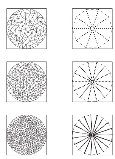
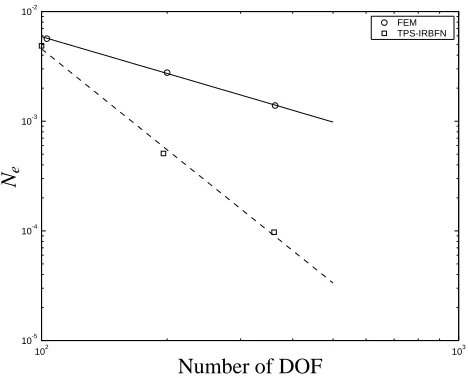
It is convenient to solve this problem in polar coordi-nates. Three discretisation schemes for both the FEM and IRBFN method are shown in Figure 8 where the RBF centres are distributed uniformly in radial and tangential directions. The representations for u and its derivatives using the second order TPS in polar coordinates are sub-stituted into (25) which is then collocated according to the set of data points chosen resulting in a linear sys-tem of equations. In order to evaluate the performance of the present IRBFN method, FEM is also employed to solve the same problem using nearly equal numbers of DOF (Figure 8 and Table 7). Note that the FEM results here are obtained using the PDE tool in MATLAB. The IRBFN method achieves a higher accuracy than the FEM (Table 7) and its convergence rate is also faster as shown in Figure 9 where the IRBFN method converges as d3.05 while the FEM only as d1.11 where d is the number of DOF.
Table 7 : Poisson’s equation on unit disk: Meshes and results by FEM and the IRBFN method.
FEM IRBFN
Nodes Triangles Ne Centres Ne
103 172 5.6653e-3 100 4.8712e−3 200 358 2.7711e-3 196 5.0875e−4 363 668 1.3985e-3 361 9.7398e−5
3.2.2 Example 2 - Jeffery-Hamel flow
102 103
10-5
10-4
10-3
10-2
FEM TPS-IRBFN
Number of DOF
[image:12.612.62.296.91.280.2]Ne
Figure 9 : Poisson’s equation on unit disk: Convergence rates by the FEM and IRBFN methods. Legends◦: FEM and2: IRBFN. The convergence rates are as d1.11 and
d3.05 for FEM and IRBFN respectively where d is the number of DOF.
discussed in many textbooks [Batchelor (1967)]. The two-dimensional steady convergent flow of a viscous, in-compressible fluid between two semi-infinite plane walls set at an angle 2αis considered here. The inward flow is driven by a steady line sink of strength Q at the apex. As pointed out by Bush and Tanner (1983), the Jeffery-Hamel flow problem provides a means of testing numer-ical solution schemes since it is a steady state flow in which the inertia terms do not vanish identically (as they do in flow between infinite parallel plates or Poiseuille flow) and an exact solution can be obtained for compari-son with numerical results. For these reacompari-sons the Jeffery-Hamel problem was used as a test example by Gartling, Nickell and Tanner (1977) in finite element convergence study, Bush and Tanner (1983) and Zheng, Phan-Thien and Coleman (1991) in boundary element convergence study. Here, this problem is also selected as a representa-tive case to assess the performance of the IRBFN method. Consider a system of polar coordinates (r,θ) centred at the point of intersection of the walls. In this coordinates system, the velocity components of the fluid are denoted as urand uθ respectively. The 2D domain of analysis is
shown in Figure 10 as a sector set at θ=±α=±π/6 with the inlet as an arc at r1and the outlet as an arc at r2.
The velocity distribution is symmetrical about the centre-lineθ=0. Owing to symmetry, only one half domain is
r1
r2 α
r
[image:12.612.365.559.166.284.2]θ
Figure 10 : Jeffery-Hamel problem: geometry.
considered. It is convenient to use the streamfunctionψ defined by
ur=−
1
r
∂ψ
∂θ, uθ=
∂ψ ∂r.
Then the vorticity can be written as
ξ=∇2ψ (33)
and for a steady, laminar and isothermal flow, the Navier-Stokes equations reduce to the vorticity equation
ρ
−1
r
∂ψ ∂θ
∂ξ
∂r+
1
r
∂ψ ∂r
∂ξ ∂θ
=µ∇2ξ, (34)
where µ is the viscosity,ρis the density and the Lapla-cian in cylindrical polar coordinates is ∇2 =∂2/∂r2+
(1/r)∂/∂r+ (1/r2)∂2/∂θ2. The no-slip condition is im-posed at the wall as
∂ψ
∂r =0,
∂ψ
∂θ =0 at θ=α,
while the symmetry condition is enforced on the centre-line, which yields
ψ=0, ξ=0 at θ=0.
At the inlet r=r1and the outlet r=r2, the boundary
in a manner consistent with the given flux Q. For conve-nience, the variables are non-dimensionlised as follows
r=rr
1, ψ
= ψ
(1/2)Q,
ui=(1/r2)Q
1 ui and ξ
= r2
1
(1/2)Qξ. (35)
From here on, the primes are dropped for brevity. The governing equations can be written as
ξ=∇2ψ, (36)
Re −1 r ∂ψ ∂θ ∂ξ
∂r +
1 r ∂ψ ∂r ∂ξ ∂θ
=∇2ξ, (37)
where Re=Q/(2ν)is the Reynolds number andν=µ/ρ
is the kinematic viscosity.
Closed form solution
In this case the domain is semi-infinite and it is not nec-essary to use the boundary conditions at the inlet and the outlet as defined by the finite size domain. Following Jef-fery and Hamel [Batchelor (1967)], the flow is assumed to be purely radial which yields self-similar velocity pro-files at all radii and, as a consequence, the streamfunction
ψdepends only onθ. Then, equation (37) gives
d4ψ dθ4 +4
d2ψ dθ2 −2Re
dψ dθ
d2ψ
dθ2 =0 (38)
subject to boundary conditions
ψ(±α) =±1 and dψ
dθ(±α) =0 (39)
for the case of full domain or,
ψ(α) =1, dψ
dθ(α) =0,ψ(0) =0,and d2ψ
dθ2(0) =0 (40)
for the case of one half domain. For this nonlinear fourth order ODE, only the closed form solution corresponding to zero or very large Reynolds numbers can be found an-alytically and hence the solution corresponding to low and medium Reynolds numbers must be solved numeri-cally. Gartling, Nickell and Tanner (1977) used an iter-ative numerical quadrature process to estimate the “ex-act” solution of Jeffery-Hamel flow. The procedure pro-vides updated approximations of the Reynolds number until the computed flux matches the prescribed flux with given values ofα,ρ,µ and the flow rate per unit length Q.
Here, the IRBFN method using second order TPS will be employed for the numerical solution of (38) and (39) and
the results obtained will be compared with the exact so-lution for two extreme cases of Reynolds number. Note that this computed IRBFN solution will be regarded as the closed form solution of the Jeffery-Hamel flow in the next section. Following are the two closed form solutions corresponding to Re=0 and Re→∞respectively. In the case of creeping flow (zero Reynolds number), equation (38) reduces to
d4ψ dθ4 +4
d2ψ
dθ2 =0 (41)
and the corresponding exact solution is
ψ= 2 cos(2α)θ−sin(2θ)
2αcos(2α)−sin(2α). (42) From (42), the ratio between the radial velocity ur and
the centreline radial velocity u0, which is independent of
radius r and the flow rate Q, can be obtained as
ur u0 =
cos(2θ)−cos(2α)
1−cos(2α) . (43)
In the case of large Reynolds number, the closed form solution was derived by Batchelor (1967)
ur u0=
3 tanh2
−1 2αRe
1
2 1−θ
α
−tanh−1 2 3 1 2
−2. (44) where Re is the Reynolds number defined as Re= αu0rρ
µ
whose value is only slightly different from the Reynolds number defined in this work. Numerical solution of the second order ODE was obtained using the MQ-IRBFN method [Mai-Duy and Tran-Cong (2001a)] where basis functions for the first derivative and the function were obtained by analytical integrations. Here, to solve higher order ODE, numerical integrations are employed to con-struct the design matrix A. In solving (38) and (39) with the presence of fourth order derivative, k={1,2,3,4} in (31) are used here to obtain basis functions for the third, second, first derivatives and the function respec-tively. Figure 11 displays the result for ur/u0 obtained
by the present IRBFN method for the case of creep-ing flow, which is in satisfactory agreement with the exact solution. The achieved norm of the relative er-ror of the solution is 7.48e−8. Results obtained for
-300 -20 -10 0 10 20 30 0.2
0.4 0.6 0.8 1
θ(degrees)
ur
/
[image:14.612.64.296.122.309.2]u0
Figure 11 : Jeffery-Hamel problem: closed form solu-tion for the case of creeping flow. Legends solid line: analytical solution and ◦: IRBFN solution. There is a good agreement between the two solutions.
0 5 10 15 20 25 30
0 0.2 0.4 0.6 0.8 1
θ(degrees)
ur
/
u0
Figure 12 : Jeffery-Hamel problem: closed form so-lution by the present IRBFN method. Legends solid line: Re=5000; dashed line: Re=1000, dashdot line:
Re=100,·: Re=50 and◦: Re=10. Result by Batch-elor (1967) at Re=5000 is also plotted with the legend +showing a good agreement with IRBFN result at large Reynolds number.
Re=5000 here. The IRBFN closed form result is in good agreement with Batchelor’s result (1967) at large Reynolds number. It can be seen that the velocity magni-tude becomes nearly constant except near the plate walls when the Reynolds number increases. On the other hand, boundary layers appear at large Reynolds number.
Computed solution
Only a finite length of the wedge geometry can be mod-elled with the IRBFN method and the boundary condi-tions at the inlet and the outlet now have to be specified for the problem. To provide a strong test for the method, the velocity vector taken from the IRBFN closed form solution is applied at the inlet while the exit condition is enforced at the outlet, i.e. ∂ψ∂r and ∂ψ∂θ at the inlet;
∂ψ ∂n =
∂ψ
∂r =0 and
∂ξ ∂n=
∂ξ
∂r =0 at the outlet where n is the
coordinate direction of the unit outward normal vector at the boundary. The flow is symmetric about the centre-line (ψ=0 and ξ=0) and no-slip conditions are pre-scribed at the plate wall (∂ψ∂r =0 and ∂ψ∂θ =0). Although the outlet boundary condition ∂ξ∂r =0 is incorrect, it can be expected that if the domain of analysis is large enough, the disturbance introduced at the outlet is small and the Jeffery-Hamel flow can be produced in the domain ex-cept for a small region at the outlet. For this reason, r1
and r2 are chosen to be 1 and 7 respectively (they were
chosen somewhat arbitrarily, but to give an aspect ratio
0 1 2 3 4 5 6 7
0 1 2 3 4
0 1 2 3 4 5 6 7
0 1 2 3 4
0 1 2 3 4 5 6 7
0 1 2 3 4
Density of 26×6
Density of 32×9
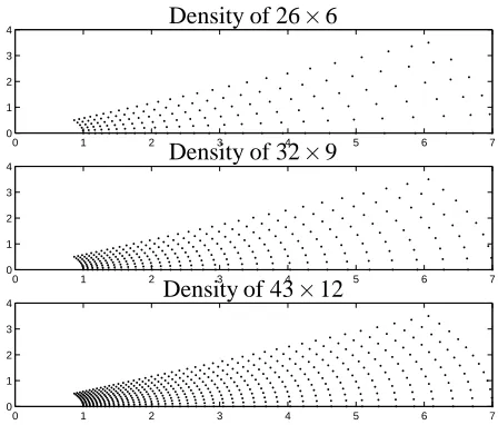
[image:14.612.63.295.413.600.2]Density of 43×12
[image:14.612.327.551.485.676.2]r2/r1which is large enough for Jeffery-Hamel flow to be
[image:15.612.324.552.125.315.2]observed and small enough to prevent the need for expen-sive calculations). Three sets of centres are displayed in Figure 13 where the discretisation is uniform in the cir-cumferential direction and non-uniform in the radial di-rection. The latter is characterised by the fact that the dis-tances between each centre and its neighbouring centres are nearly equal. Iterative procedure is employed to cope with the nonlinear convective term which is similar to the iterative procedure described in section 2.3.3. The con-vective term is estimated using the result at the previous iteration and hence this term becomes known at the cur-rent iteration resulting in a linear least-squares problem. Note that by using this approach the design matrix A does not change during iteration and hence the SVD algorithm for A needs to be done only once. Furthermore, this de-composition can be used for any Reynolds number due to the fact that A does not depend on the material properties. For this problem, numerical experience shows that the first order TPS achieves a better results than the second order TPS and the results corresponding to the former are presented. With three relatively coarse centre den-sities employed, the IRBFN method can achieve moder-ate Reynolds numbers. The solution is convergent up to Reynolds numbers of 100, 150 and 200 with discretisa-tions in tangential direction only being 6, 9 and 12 points (6, 3.75 and 2.5 degrees) respectively. It can be seen that at the Reynolds number of 200 the profile of the radial velocity is very steep near the wall. Higher Reynolds number will produce the boundary layer and a number of discretisation points in the tangential direction needs to be increased resulting in relatively large matrices. In this case it is better to use the domain decomposition tech-nique rather than the single domain, which is to be re-ported in future work. The results including the variation of the radial velocity along the centreline and the pro-file of the radial velocity at r≈3.5 (roughly half way between the inlet and the outlet) are displayed in Fig-ures 14-19 from which it can be seen that the agreement with the closed form solution is satisfactory. The IRBFN method can achieve Reynolds number up to Re=200
us-ing 12 points distributed uniformly in tangential direction in comparison with Re up to 40 using 11 points achieved by BEM [Zheng, Phan-Thien and Coleman (1991)] and
Re up to 1000 using 21 points by FEM [Gartling, Nickell
and Tanner (1977)].
1 2 3 4 5 6 7
0.2 0.4 0.6 0.8 1 1.2 1.4 1.6 1.8 2 2.2
closed form IRBFN
r
u0
Figure 14 : Jeffery-Hamel problem, centre density of 26×6: the radial velocity obtained along the centreline at Re=100
0 5 10 15 20 25 30
0 0.2 0.4 0.6 0.8 1
closed form Re=10 Re=50 Re=100
θ(degrees)
ur
/
[image:15.612.322.553.439.642.2]u0
1 2 3 4 5 6 7 0.2
0.4 0.6 0.8 1 1.2 1.4 1.6 1.8 2 2.2
closed form IRBFN
r
[image:16.612.321.552.126.315.2]u0
Figure 16 : Jeffery-Hamel problem, centre density of 32×9: the radial velocity obtained along the centreline at Re=150
0 5 10 15 20 25 30
0 0.2 0.4 0.6 0.8 1
closed form Re=10 Re=50 Re=100 Re=150
θ(degrees)
ur
/
[image:16.612.67.300.127.315.2]u0
Figure 17 : Jeffery-Hamel problem, centre density of 32×9: the profile of radial velocity at r ≈ 3.5 for Reynolds numbers of 10, 50, 100 and 150.
1 2 3 4 5 6 7
0.2 0.4 0.6 0.8 1 1.2 1.4 1.6 1.8 2
closed form IRBFN
r
[image:16.612.320.552.455.642.2]u0
Figure 18 : Jeffery-Hamel problem, centre density of 43×12: the radial velocity obtained along the centreline at Re=200
0 5 10 15 20 25 30
0 0.2 0.4 0.6 0.8 1
closed form Re=10 Re=50 Re=100 Re=200
θ(degrees)
ur
/
u0
[image:16.612.65.295.457.642.2]4 Concluding remarks
In this paper, the Indirect RBFN method using first and second order thin plate splines for numerical solu-tion of DEs in rectangular and curvilinear coordinates is developed and verified successfully. Special attention here is given to the employment of numerical integra-tion schemes in the IRBFN procedure where new basis functions for lower derivatives and function could not be found explicitly by analytical integrations. This scheme allows the indirect RBFN method to be general in the sense that the method can be employed with any kind of radial basis function and also in any kind of coordi-nates system. Furthermore, the scheme is also effective in solving higher DEs, i.e. there are no added compu-tational difficulties relative to the case of second order DEs. Gaussian quadrature is employed throughout the study and the results obtained are accurate. The TPS-IRBFN is easy to implement and more automatic than the MQ-IRBFN method and numerical examples show that the TPS-IRBFN method achieves a high accuracy.
Acknowledgement: This work is supported by a Spe-cial USQ Research Grant (Grant No 179-310) to Thanh Tran-Cong. Nam Mai-Duy is supported by a USQ schol-arship. This support is gratefully acknowledged. The authors would like to thank the referees for their helpful comments.
References
Abramowitz, M.; Stegun, I. A. (1972): Handbook of
Mathematical functions. Dover Publications, New York.
Atluri, S. N.; Shen, S. (2002a): The meshless lo-cal Petrov-Galerkin (MLPG) method: A simple & less-costly alternative to the finite element and boundary ele-ment methods. CMES: Computer Modeling in
Engineer-ing & Sciences, vol. 3, pp. 11-52.
Atluri, S. N.; Shen, S. (2002b): The Meshless Local
Petrov-Galerkin Method. Tech Science Press, Encino.
Batchelor, G. K. (1967): An Introduction to Fluid
Dy-namics. Cambridge University Press, Cambridge.
Bjorck, A. (1996): Numerical Methods for Least Squares Prolems. SIAM, Philadelphia.
Bush, M. B.; Tanner, R. I. (1983): Numerical solution of viscous flows using integral equation methods.
Inter-national Journal for Numerical Methods in Fluids, vol.
3, pp. 71-92.
Dissanayake, M. W. M. G.; Phan-Thien, N. (1994): Neural-Network-Based approximations for solving par-tial differenpar-tial equations. Communications in Numerical
Methods in Engineering, vol. 10, pp. 195-201.
Dubal, M. R. (1994): Domain decomposition and local refinement for multiquadric approximations. I: Second-order equations in one-dimension. Journal of Applied
Science and Computation, vol. 1(1), pp. 146-171.
Duchon, J. (1977): Splines minimizing rotation-invariant semi-norms in Sobolev spaces. In: W. Schempp and K. Zeller (eds) Constructive Theory of Functions
of Several Variables, Lecture Notes in Mathematic,
Springer-Verlag, Berlin, vol. 571, pp. 85-100.
Fornberg, B.; Driscoll, T. A.; Wright, G.; Charles, R. (2002): Observations on the behavior of radial ba-sis function approximations near boundaries. Computers
and Mathematics with Applications, vol. 43, pp.
473-490.
Gartling, D. K.; Nickell, R. E.; Tanner, R. I. (1977): A finite element convergence study for accelerating flow problems. International Journal for Numerical Methods
in Engineering, vol. 11, pp. 1155-1174.
Gutmann, H. M. (2001): On the semi-norm of radial ba-sis function interpolants. Journal of Approximation
The-ory, vol. 111, pp. 315-328.
Haykin, S. (1999): Neural Networks: A Comprehensive
Foundation. Prentice-Hall, New Jersey.
Ingber, M. S.; Phan-Thien, N. (1992): A boundary el-ement approach for parabolic differential equations us-ing a class of particular solutions. Applied Mathematical
Modelling, vol. 16, pp. 124-132.
Kansa, E. J. (1990): Multiquadrics- A scattered data ap-proximation scheme with applications to computational fluid-dynamics-II. Solutions to parabolic, hyperbolic and elliptic partial differential equations. Computers and Mathematics with Applications, vol. 19(8/9), pp.
147-161.
Mai-Duy, N.; Tran-Cong, T. (2001a): Numerical so-lution of differential equations using multiquadric radial basis function networks. Neural Networks, vol. 14, pp. 185-199.
Numerical Methods in Fluids, vol. 37, pp. 65-86.
Mai-Duy, N.; Tran-Cong, T. (2002): Mesh-free radial basis function network methods with domain decompo-sition for approximation of functions and numerical so-lution of Poisson’s equations. Engineering Analysis with
Boundary Element, vol. 26, pp. 133-156.
Press, W. H.; Flannery, B. P.; Teukolsky, S. A.; Vetter-ling, W. T. (1988): Numerical Recipes in C: The Art of
Scientific Computing. Cambridge University Press,
Cam-bridge.
Schaback, R. (1995): In: M. Daehlen; T. Lyche and L. L. Schumaker (eds) Mathematical Methods for Curves
and Surfaces, Vanderbilt University Press, Nashville, pp.
477-496.
Sharan, M.; Kansa, E. J.; Gupta, S. (1997): Applica-tion of the multiquadric method for numerical soluApplica-tion of elliptic partial differential equations. Journal of Applied
Science and Computation, vol. 84, pp. 275-302.
Takeuchi, J.; Kosugi, Y. (1994): Neural network rep-resentation of finite element method. Neural Networks, vol. 7(2), pp. 389-395.
Zerroukat, M.; Power, H.; Chen, C. S. (1998): A nu-merical method for heat transfer problems using colloca-tion and radial basis funccolloca-tions. Internacolloca-tional Journal for
Numerical Methods in Engineering, vol. 42, pp.
1263-1278.
Zerroukat, M.; Djidjeli, K.; Charafi, A. (2000): Ex-plicit and imEx-plicit meshless methods for linear advection-diffusion-type partial differential equations. Interna-tional Journal for Numerical Methods in Engineering,
vol. 48, pp. 19-35.
Zheng, R.; Phan-Thien, N.; Coleman, C. J. (1991): A boundary element approach for non-linear boundary-value problems. Computational Mechanics, vol. 8, pp. 71-86.