Theses
11-27-2018
Resiliency in Deep Convolutional Neural
Networks
Faiz Ur Rahman
Follow this and additional works at:https://scholarworks.rit.edu/theses
Recommended Citation
Resiliency in Deep Convolutional Neural Networks
Resiliency in Deep Convolutional Neural Networks
Faiz Ur Rahman
November 27, 2018
A Thesis Submitted in Partial Fulfillment
of the Requirements for the Degree of Master of Science in Computer Engineering
Resiliency in Deep Convolutional Neural Networks
Faiz Ur Rahman
Committee Approval:
_____________________________________________Date:______________
Dr. Andreas Savakis
Primary Advisor – Professor, R.I.T. Dept. of Computer Engineering
_____________________________________________Date:______________
Dr. Andres Kwasinski
Committee Member – Professor, R.I.T. Dept. of Computer Engineering
_____________________________________________Date:______________
Dr. Dhireesha Kudithipudi
Acknowledgements
I would like to thank the Visual Image Processing Lab of Rochester Institute of
Technology (RIT) for providing me the resources as well as inspiration to
complete this thesis, my adviser Dr. Andreas Savakis for his patience and
assisting me throughout my thesis, my colleague and friend Mr. Bhavan Vasu
for his valuable feedback. I would like to thank Dr. Dhireesha Kudithipudi and Dr.
Andres Kwasinski for serving as my committee members and for their time and
effort in supporting my research. I would like to thank everyone in Computer
To my loving parents, sister and brother in law for endless support throughout my
masters no matter what the situation is on their end and for believing in me.
To my friends Chandini Ramesh, Saurabh Chatterjee and Chinmay Kulkarni who stood
Abstract
The enormous success and popularity of deep convolutional neural networks
for object detection has prompted their deployment in various real world
applications. However, their performance in the presence of hardware faults or
damage that could occur in the field has not been studied. This thesis explores
the resiliency of six popular network architectures for image classification,
AlexNet, VGG16, ResNet, GoogleNet, SqueezeNet and YOLO9000, when
subjected to various degrees of failures. We introduce failures in a deep network
by dropping a percentage of weights at each layer. We then assess the effects of
these failures on classification performance. We find the fitness of the weights
and then dropped from least fit to most fit weights. Finally, we determine the
ability of the network to self-heal and recover its performance by retraining its
healthy portions after partial damage. We try different methods to re-train the
healthy portion by varying the optimizer. We also try to find the time and
Table of Contents
Signature Page ... i
Acknowledgements ... ii
Abstract ... iv
List of Figures ... vii
List of Tables ... ix
Acronyms ... x
Chapter 1 ... 2
Introduction ... 2
1.1 Motivation ... 2
1.2 Literature Review ... 4
1.3 Contribution ... 6
1.4 Thesis Organization ... 7
Chapter 2 ... 9
Materials ... 9
2.1 Dataset ... 9
2.1.1 MS COCO ...9
2.1.2 AID ...10
2.2 Methods ... 11
2.2.1 AlexNet ...12
2.2.2 VGG16 ...14
2.2.3 ResNet ...16
2.2.4 GoogleNet ...18
2.2.5 SqueezeNet ...19
2.2.6 YOLO ...20
Chapter 3 ... 23
Proposed Methods ... 23
3.1 Training the CNN’s ... 23
3.1.1 Training AlexNet ...24
3.3 Resiliency in DCNN’s ... 33
3.3.1 Resiliency with faults across the network ...34
3.3.1.1 Dropping weights using in-built function ... 35
3.3.1.2 Dropping weights manually ... 36
3.3.2 Resilience with faults at a single convolution layer ...37
3.3.3 Resilience with faults across the entire network with fitness ...38
3.3.3.1 Taylor Ranking ... 39
3.4 Self-Healing by Re-training ... 40
3.4.1 Re-training with AdaGrad ...41
3.4.2 Re-training with Adadelta ...42
3.4.3 Re-training with Rprop ...43
3.4.4 Re-training with ADAM optimizer ... 44
3.4.5 Retraining with ARprop ...45
3.5 Pruning ... 47
Chapter 4 ... 49
Results ... 49
4.1 Resiliency with faults across the network ... 49
4.2 Resilience with faults at a single convolution layer ... 55
4.3 Resilience with faults across the entire network with fitness ... 58
4.4 Network Self-Healing by Retraining ... 60
4.4.1 Retraining with AdaGrad Optimizer ...60
4.4.2 Retraining with AdaDelta Optimizer ...67
4.4.3 Retraining with Rprop Optimizer ...72
...76
4.4.4 Retraining with ADAM Optimizer ...76
4.5 Retraining with ARprop ...82
4.5 Dataset for Re-training ... 87
4.6 Pruning ... 88
Chapter 5 ... 89
Conclusion ... 89
List of Figures
Figure 2.1 MSCOCO 2014 dataset ... 10
Figure 2.2 AID Dataset ... 11
Figure 2.3 AlexNet architecture ... 13
Figure 2.4 VGG16 Architecture [41] ... 15
Figure 2.5 ResNet Architecture [42] ... 17
Figure 2.6 GoogleNet Architecture [43] ... 18
Figure 2.7 SqueezeNet Architecture [45] ... 19
Figure 2.8 YOLO Architecture ... 21
Figure 3.1 Illustration of how weight damage (red) is introduced into the network architecture. ... 34
Figure 3.2 Toy example of weights (a) Represents weights before drop and (b) Represents weights after drop ... 36
Figure 3.3 Illustration of how weight damage (red) is introduced into the network architecture ... 38
Figure 3.4 Network Pruning flow diagram ... 47
Figure 4.1 Accuracy vs Percent of Dropped Weights across the full network in AlexNet, VGG16 and ResNet ... 50
Figure 4.2 Accuracy vs Percent of Dropped Weights across the full network in SqueezeNet, GoogleNet and YOLO. ... 52
Figure 4.3 Accuracy vs Percentage of dropped weights across the full network comparing ResNet and YOLO ... 53
Figure 4.4 ccuracy vs Percentage of dropped weights across the full network comparing VGG16 and GoogleNet ... 54
Figure 4.5 Accuracy vs Percentage of dropped weights across the full network for all the architecture ... 55
Figure 4.6 Accuracy vs Percent of Dropped Weights in last convolution layer for AlexNet (red), VGG (green), and ResNet ... 56
Figure 4.7 Accuracy vs Percent of Dropped Weights in last convolution layer for SqueezeNet (red), YOLO(blue), and GoogleNet(green) ... 57
Figure 4.8 Accuracy vs percentage drop in AlexNet, VGG16 and ResNet with fitness .. 58
Figure 4.9 Accuracy vs percentage drop in SqueezeNet, GoogleNet and YOLO with fitness ... 59
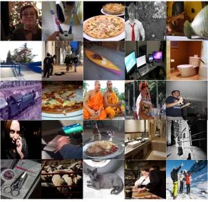
GoogleNet, YOLO ... 63 Figure 4.13 Examples of correct and incorrect classification after 50% of dropped
weights when re-trained with AdaGrad ... 65 Figure 4.14 Examples of correct and incorrect classification after 25% of dropped
weights when re-trained with AdaGrad ... 66 Figure 4.15 Performance recovery by retraining (self-healing) after weights are dropped
throughout the a) AlexNet, VGG16, ResNet, b)SqueezeNet, GoogleNet, YOLO .... 67 Figure 4.16 Performance recovery by retraining (self-healing) after weights are dropped
with fitnetss throughout the a) AlexNet, VGG16, ResNet, b)SqueezeNet,
GoogleNet, YOLO ... 68 Figure 4.17 Examples of correct and incorrect classification after 50% of dropped
weights when re-trained with AdaDelta ... 69 Figure 4.18 Examples of correct and incorrect classification after 25% of dropped
weights when re-trained with AdaDelta ... 71 Figure 4.19 Performance recovery by retraining (self-healing) after weights are dropped
throughout the a) AlexNet, VGG16, ResNet, b)SqueezeNet, GoogleNet, YOLO .... 72 Figure 4.20 Performance recovery by retraining (self-healing) after weights are dropped
with fitnetss throughout the a) AlexNet, VGG16, ResNet, b)SqueezeNet,
GoogleNet, YOLO ... 73 Figure 4.21 Examples of correct and incorrect classification after 50% of dropped
weights when re-trained with Rprop ... 75 Figure 4.22 Examples of correct and incorrect classification after 25% of dropped
weights when re-trained with Rprop ... 76 Figure 4.23 Performance recovery by retraining (self-healing) after weights are dropped
throughout the a) AlexNet, VGG16, ResNet, b)SqueezeNet, GoogleNet, YOLO .... 77 Figure 4.24 Performance recovery by retraining (self-healing) after weights are dropped
with fitnetss throughout the a) AlexNet, VGG16, ResNet, b)SqueezeNet,
GoogleNet, YOLO ... 78 Figure 4.25 Examples of correct and incorrect classification after 50% of dropped
weights when re-trained with ADAM optimizer ... 79 Figure 4.26 Examples of correct and incorrect classification after 25% of dropped
weights when re-trained with ADAM optimizer ... 81 Figure 4.27 Performance recovery by retraining (self-healing) after weights are dropped
throughout the a) AlexNet, VGG16, ResNet, b)SqueezeNet, GoogleNet, YOLO .... 82 Figure 4.28 Performance recovery by retraining (self-healing) after weights are dropped
with fitnetss throughout the a) AlexNet, VGG16, ResNet, b)SqueezeNet,
List of Tables
Table 2-1 Features of each of the Neural Network architectures ... 12 Table 3-1 Parameters required for training each of the six algorithms ... 24 Table 4-1 Network parameters and associated test accuracy with 50% faults across the
entire network ... 64 Table 4-2 Network parameters and associated test accuracy with 25% faults across the
entire network ... 64 Table 4-3 Network parameters and associated test accuracy with 50% faults across the
entire network ... 68 Table 4-4 Network parameters and associated test accuracy with 25% faults across the
entire network ... 69 Table 4-5 Network parameters and associated test accuracy with 50% faults across the
Network ... 73 Table 4-6 Network parameters and associated test accuracy with 25% faults across the
Network ... 74 Table 4-7 Network parameters and associated test accuracy with 50% faults across the
Network ... 78 Table 4-8 Network parameters and associated test accuracy with 25% faults across the
Network ... 79 Table 4-9 Network parameters and associated test accuracy with 50% faults across the
Network ... 84 Table 4-10 Network parameters and associated test accuracy with 25% faults across the
Network ... 84 Table 4-11 Network Parameters, with its associated accuracy and number of iterations
2D
Two-dimensional
AdaGrad
Adaptive Gradient Descent
AID
Aerial Image Dataset
ANN
Artificial Neural Network
ARprop
ADAM Resilient Propagation
ADAM
Adaptive Moment Estimation
AlexNet
Alex Network
CNN
Convolutional Neural Network
DCNN
Feed Forward Dense Network
GoogleNet
Google Network
MSCOCO
Microsoft Common Objects in Context
PCA
Principal Component Analysis
RMS
Root Mean Square
ReLU
Rectified Linear Unit
ResNet
Residual Neural Network
Rprop
Resilient Propagation
SqueezeNet
Squeeze Network
VGG
Visual Geometry Group
Chapter 1
Introduction
1.1 Motivation
Deep Convolutional Neural Networks (DCNNs) have become the golden standard for
object detection and localization and are increasingly adopted for various applications
including face recognition [1], autonomous vehicles [2] and medical diagnosis [3]. The
combination of Artificial Neural Network and convolution led to solving of object
recognition and other computer vision related problems that was first accomplished by
AlexNet [4] architecture on ImageNet [5] challenge which incited research in deep
field of computer vision especially for object recognition tasks. Over time deeper and
much more efficient architectures were introduced for object detection tasks like
Faster-RCNN [9] and YOLO [10] [11]. With the increase in depth of Convolutional Neural
Networks increased the demand for larger GPU’s, to reduce this, smaller architectures
like SqueezeNet [12] started taking the place of these larger architectures which were
more suitable for mobile or embedded platform. There is also a trend in pruning the
network architecture to reduce its computations which makes training easier and
faster. This was first achieved by DenseNet [13] architecture which used half the
number of parameters as VGG without sacrificing its performance. A comprehensive
study on network speed-accuracy tradeoffs is presented in [14].
CNNs have turned out to be powerful in analyzing images and detecting objects of
interest. One of the significant advantages of CNN’s is the end to end learning of
features with a classifier, giving it leeway over conventional feature extractors paired
with classifiers. The limitation of CNNs lies in their requirement of immense training
datasets making it computationally costly. Deep learning frameworks, such as Caffe
[15], Torch [16], Tensorflow [17] and PyTorch [18], have enabled training with the
assistance of GPUs and have made the learning process considerably more effective.
Transfer learning is a strategy used to learn new layer weights in neural network for a
given dataset from a pertrained model using a standard dataset.
With the increasing use of DCNNs in real world situations, hardware or embedded
implementation are placed in environments where they could suffer damage due to
hardware failure like memory failure [19] or harsh external conditions or software
attacks like Malware attack which is a cyber-attack that performs operations on victim’s
computer without their knowledge [20] or bit-flipping, where the attacker can change
the ciphertext without the knowledge of the owner [21]. However, to our knowledge,
the performance of DCNNs under failure conditions has not been investigated. The
objective of this thesis is to explore the resilience of six popular object detector network
architectures, AlexNet [4], VGG [6], ResNet [8], SqueezeNet [12], GoogleNet [7] and
YOLO [10] [11] [22], when subjected to various degrees of failure.
A potential form of failure in a DCNN is due to corruption of network weights. This
type of corruption could occur at few or many nodes in the network, and is likely to
result in misclassification and leading to deterioration in performance.
There is limited research on the performance of deep networks under various types of
faults. The most relevant research is reported in [23] and [24]. In [23] the effects of
coefficient quantization on network performance is examined for fixed point
implementations.
In [24] examining the resilience of the network is done by dropping features randomly
using a stress function (TDR-1) and performing Principal Component Analysis (PCA)
which keeps the most significant features along the direction of maximum variance.
The stress function is passed through the network with frozen layers and trained on
SVM classifier. In addition to TDR-1, Q-2 feature compression due to quantization is
applied simultaneously. The difference between quantization and stress is that
quantization just tampers the numerical precision of representation [25], while stress
refers to dropping the weights randomly. In [19] resiliency is explored by bit level fault
injection, which imitates the faults at the hardware level i.e. memory while training and
testing. The weight file is modified while training which is called static injection of
errors and while testing which is called dynamic injection of faults. Whereas, our
experiments involve different ways of dynamic injection of faults. Our contributions
go well-beyond the work in [24], [23] and [19], by methodically examining the effects
of faults in six different architectures and retraining the networks to recover some of
The brute force ranking method is to prune each layer, and observe how the cost
changes when running on the training set. This is known as oracle ranking, the most
ideal ranking of filters for limiting the system cost change. Presently to quantify the
performance of other training techniques, pruning a filter is the equivalent to zeroing
it out [26]. The ranks are then normalized [27].
The resilient propagation (Rprop) has been very popular for FFDN training [28]. FFDN
refers to feed forward neural network where connections between the neurons do not
form a loop. Combining dropout with Rprop proved to be more effective and started
giving better results [29]. Rprop considers only the sign of the gradient for its weight
updating independently for each of the parameters [30]. By independently, each
parameter will have its own step size. So, instead of updating with the magnitude of
the gradient, it updates with the step size that is defined for that weight. That step size
adapts individually over time to accelerate learning in the direction needed [31]. This
method is much faster than standard SGD backpropagation.
1.3 Contribution
1. We provide a quantitative assessment of the DCNN object detector performance
due to partial failures.
2. We gain understanding of the effects of faults at various locations in the DCNN's
hidden layers.
3. We explore that DCNN’s can be of optimal depth without having to compromise
performance i.e. we can remove few layers without compromising performance.
4. We explore that DCNN’s can have fewer parameters (weights) without having to
compromise performance.
5. We demonstrate that resiliency of DCNN’s are dependent on the architecture and
not the datasets.
6. We demonstrate that Rprop is the best retraining technique for healing the network.
7. We demonstrate that DCNN’s can self-heal to overcome the effects of faults by
retraining the healthy parts of the network.
8. We propose a technique for pruning DCNN’s to the desirable depth for a given
problem [32].
9. We explore the effects of dataset size required for re-training.
1.4
Thesis Organization
mentioned below:
• Chapter 1. Introduction: This chapter gives a brief introduction to the topic of
thesis, motivation behind this thesis followed by a literature review of
previous work in this field finally the contribution of the thesis.
• Chapter 2.Materials: This chapter starts by describing the datasets that are
used in this thesis in detail, followed by a detail description of convolutional
neural network architecture used in this thesis.
• Chapter 3. Proposed Methods: This chapter starts with description of
resiliency and how the network has been trained, followed by dropping of
weights with and without computation of fitness of the neuron. The next
section describes how the network can heal itself by re-training by using
different methods. The last section is pruning VGG16 and GoogleNet to the
size of SqueezeNet.
• Chapter 4. Results: This chapter describes how the each of CNN’s act when
subjected to damages followed by how fast each of these networks can heal
itself after the introduction of failure. This chapter also has results for pruning
VGG16 and GoogleNet.
Chapter 2
Materials
This chapter starts by describing the datasets that are used in this thesis in detail
followed by a detailed description of the convolutional neural network architectures
used in this thesis.
2.1 Dataset
2.1.1 MS COCO
COCO stands for Common Objects in Context [33]. As indicated by the name, images
in the COCO dataset are taken from regular scenes and includes labels for the objects
in the images. The dataset contains images of 91 objects types with a total of 2.5 million
dataset.
Figure 2.1 MSCOCO 2014 dataset
2.1.2 AID
AID is an aerial image dataset [34]. A few examples are shown in Fig. 2.2. AID dataset
consists of 30 classes including airport, railway track, waterbody and so on and total of
multi-images per each class in AID are collected from different regions, for the most part in
China, the United States, England, France, Italy, Japan, Germany, and so on. They are
taken at various times and seasons under various imaging conditions, which expands
[image:24.612.155.458.236.488.2]the intra-class variability.
Figure 2.2 AID Dataset
There are six different popular convolutional neural network architectures that have
been used for training. The description and the architecture of each architecture is
described in this section. The architectures considered in this thesis are AlexNet,
VGG16, ResNet, GoogleNet, SqueezeNet and YOLO architecture. Table 2.1 shows
some features of all the six architectures. The architecture of each of these networks is
described below.
Table 2-1 Features of each of the Neural Network architectures
Networks Maximim Filter size Minimum Filter size Blocks Inception Residual/
blocks
FC
layers Hidden layers
AlexNet 11X11 3X3 0 0/0 3 6
VGG16 3X3 3X3 5 0/0 3 14
ResNet 7X7 3X3 25 25/0 1 48
GoogleNet 5X5 1X1 9 0/9 1 20
SqueezeNet 3X3 1X1 8 0/8 0 16
YOLO 3X3 1X1 23 23/0 1 51
2.2.1 AlexNet
AlexNet was an innovative architecture to tackle large labeled datasets for image
recognition with higher precision and efficiency. The ImageNet dataset used to train
better scalability and faster training. Hence leveraging a multi GPU system can
speed-up training as well as evaluation for large datasets. AlexNet set the premise to better
image classification architectures and research using deep learning techniques and
methods. Fig. 2.3 shows the architecture of AlexNet.
Figure 2.3 AlexNet architecture
The architecture for the Alexnet contains 5 convolution neural layers and 3
fully-connected layers. The architecture of AlexNet used ReLU [37] [38] activation function
in its neural layers to accommodate faster training over traditional activation functions
like tanh [39]. The response to normalization of layer’s average data given during
training to prevent stagnant learning iterations and high false positives in recognition.
The max pooling layers helped reduce variance also capturing strong inputs over the
network layers. Pooling layers are placed after the response normalization layers. The
The convolutional layers are split to contain mapped kernels in the same graphical
processing units. The convolutional layers reduce the image parameters producing
4096 dimensional features for the fully connected (FC) layer that are mapped into a
logistic regression output containing 1000 classes.
This architecture uses various kinds of transformations for data augmentation to
increase learning. These spatial transforms provide more robust training samples for
the network.
2.2.2 VGG16
VGGNet is a neural network that performed extremely well in the Image Net Large
Scale Visual Recognition Challenge (ILSVRC) in 2014. This architecture is from VGG
group, Oxford. It makes the enhancement over AlexNet by replacing expensive
kernel-size filters with various 33 filters in a steady progression. Fig. 2.4 shows the VGG16
architecture. This idea of blocks/modules was introduced in VGG. The VGG
convolutional layers are trailed by 3 fully connected layers. The width of the filters
The images in the challenge were divided into 1000 unique classes. Given a test image,
the VGG network determines a likelihood — in the range of 0 and 1 — for every one of
those 1000 classes and selects the class with the highest likelihood.
2.2.3 ResNet
With the advent of deep learning in various areas of research important applications
were found. The major drawback of deep learning networks is the size of dataset
required to train them along with the hyper parameters associated with them. Other
issues include losing the learning capability due to extensive stacking of layers and
overfitting. The research on residual networks was premised on tackling the problem
of vanishing gradients and training efficiency between layers. The residual blocks
provide mappings that preserves the transformations in the previous layers.
The architecture for ResNet illustrated in Fig. 2.5 adds identity mappings known as
skip connections. These skip connections decide the depth of the neural network
depending on the dataset. The network first starts training with one residual block and
keeps adding the new layers by checking gradient. There is no problem of dimensional
mismatch as all the filters in all the layers are of the same size. The only problem that
can be inherited is the number of filters in the layer and input to the next layer. To
overcome this, it uses same padding. The architecture consists of 3x3 filters with 2
Figure 2.6 GoogleNet Architecture [43]
2.2.4 GoogleNet
The GoogleNet model, shown in Fig. 2.6, contains an essential block called inception
block containing progressions of convolutional layers at various scales. For every block,
we take in an arrangement of 1x1, 3x3, and 5x5 filters which can figure out how to
extract features at various scales from the image. Max pooling is additionally utilized,
yet with same padding to have a legitimate connection while concatenating features
from the three filters [43].
The GoogleNet architecture consists of 9 inception blocks. The easiest way to improve
the performance of the deep learning model is by adding more layers and increasing
the data. With more parameters, the network is prone to overfit. To avoid overfitting
Figure 2.7 SqueezeNet Architecture [45]
2.2.5 SqueezeNet
SqueezeNet proposes an efficient architecture that gives accuracy that is similar to
smaller than AlexNet. The building block of SqueezeNet is called fire module, which
consists of a squeeze layer and an expand layer. A SqueezeNet stacks a group of fire
modules and a pooling layer after a couple of fire module. The squeeze layer reduces
the feature map size and expand layer increases it, thus helps to keep the original
feature map size [45].
In Fig. 2.7, the squeeze module just contains 1x1 filters, which means it works like a
fully connected layer. As its name indicates, one of its benefits is to decrease the size of
the feature map. Diminishing size implies that there are fewer calculations to do in the
accompanying 3x3 channels. It helps the speedup as a 3x3 filters require multiple more
calculations compared to a 1x1 channel [45].
2.2.6 YOLO
The YOLOV3 network architecture consist of fifty two convolutional layers followed
by an average pooling layer and one fully connected layer making it a total of fifty
layers with 50 hidden layers. The 52 convolutional layer is divided into five residual
blocks which are repeated several times as can be seen in the Fig. 2.8. Unlike most
Figure 2.8 YOLO Architecture
The complexity of architecture is directly proportional to the depth of the convolutional
evidence that residual networks with the inclusion of dropout is much faster to train.
Residual networks show significant improvements on ImageNet and MSCOCO
dataset. The residual network may have deeper layers compared to its counterparts,
but because of skip connections the active parameters are lesser than non-residual
Chapter 3
Proposed Methods
This chapter describes how the networks have been trained from pre-trained models
available in Caffe zoo. Then it describes how the weights have been dropped to
determine the resiliency of the neural network, and includes self-healing of all the
DCNN’s after the weights have been dropped by different methods before re-training.
We also prune the most resilient networks like VGG16 and GoogleNet to the size of
SqueezeNet and compare its results.
3.1 Training the CNN’s
The Deep Convolutional Neural Networks were built from scratch in Keras and
PyTorch, i.e. instead of taking the model from the library in Keras, each of these neural
no access to perform changes within the network. This also provided a deeper
understanding of the architecture. Table 3.1 shows parameters requires for training
different architectures.
Table 3-1 Parameters required for training each of the six architectures
Network AlexNet VGG16 ResNet SqueezeNet GoogleNet YOLO
Built from
scratch Yes Yes Yes Yes Yes Yes
Weights Model Caffe
Zoo
Caffe Model
Zoo
Caffe Model
Zoo
Caffe Model
Zoo Caffe Model Zoo website YOLO
Layers Replaced layers 3 FC layers 2 FC
1 FC layers
and 1 residual
block
1 Convolution
Layer 1 FC layer layer 1 FC
Regularization No Yes Yes (FC Layer) No Yes No
Learning Rate 0.01 0.01 0.0001 0.01 0.01 0.001
Loss Entropy Cross- Entropy Cross- Entropy Cross- Squared ErrorMean Squared Mean
Error YOLO
Optimizer ADAM SGD ADAM SGD AdaGrad ADAM
3.1.1 Training AlexNet
used directly in Keras (with TensorFlow in the background). Luckily there is a tool [47]
available online which can be used to convert this weight file to .h5 file which is
compatible with Tensorflow. This tool maps the weights to the dimension of the filter.
The tool updates the weights in the tensor format to form an nd-array of values which
then stored as a file in .h5 format. These weights are uploaded in python using.
load_weights. The loaded weights are pre-trained weights, which have been
previously trained on the ImageNet dataset. As ImageNet and MsCOCO dataset are
not that different from each other, we can assume the network features will be similar
to the features required by the classifier for MSCOCO dataset.
The pre-trained weights are trained on ImageNet dataset which has 1000 classes and
hence, once we upload the weights and match it with the AlexNet model, our network
is ready to classify 1000 objects. For transfer learning on the MSCOCO dataset, we
remove the FC layers from the network and replace it with a new FC layer which has
never been trained.
The next step is to train the new FC layers with the new dataset that can classify 10
object classes so its output will be 10 classes instead of 1000 classes. The loss used for
training is cross-entropy loss and the optimizer used for training the network is ADAM
3.1.2 Training VGG16
VGG16 is a straight-forward architecture and can be implemented in Keras by using
“Api” model and adding layers with its respective filter size. The pre-trained weights
are taken from caffe model zoo. We follow the same procedure as described in in
Section 3.1.1.
Again, the weights have been pre-trained on the ImageNet dataset. During transfer
learning, we are not training the first few layers, as they just give simple features that
are commonly found across datasets.
As VGG16 has a lot of parameters and hidden layers, it is prone to overfitting during
transfer learning on the MSCOCO dataset. We follow three steps to train this network.
First, we remove all the FC layers and add new FC layers that are connected to the last
convolution layer of VGG1. Then all the hidden layers are frozen (set to non-trainable)
The next step is to regularize this overfit model by adding dropout layer (which act as
an adaptive regularization technique) [35]. A dropout layer is added after each FC layer
(which drops random weights after each iteration). As was done in the first step, all the
hidden layers are frozen while the FC layers are trained with dropout.
The next step is to finetune the network by training it end to end just for a couple of
epochs. This is done by making all the hidden layers trainable and removing all the
dropout layers in the network, so all the layers in VGG16 are now trainable (can update
its weights while back-propagating) [48].
The hyper parameters used in this training is SGD optimizer [49], with learning rate set
to default i.e. 0.01 and using cross entropy loss [50].
3.1.3 Training ResNet
ResNet is a complex architecture and can be implemented in keras by having the
residual connections and letting the network decide its own depth. The pre-trained
weights are taken from caffe model zoo and converted to .h5 format using convert.py
The pre-trained weights are trained on ImageNet dataset by the authors of ResNet.
These weights are trained to classify 1000 object classes. Again we perform transfer
learning by replacing the last Fully Connected layer to output 10 classes as we did in
previous networks. However, AlexNet and VGG16 have two fully connected layers
which learn to classify objects in the image but ResNet has only one fully connected
layer to give 10 class output. If just the one fully connected layer is trained then the
network will learn very fast and it may skip the local minima.
This above stated problem can be overcome by including more layers for training and
not just the fully connected layer. With this process, the learning parameters will have
a lot more weights to update, so the learning pace is not that fast and it can converge
correctly. The ResNet model’s last residual block and the Fully connected layer is now
trained on MSCOCO dataset for classify 10 class objects by using dropouts in the Fully
connected layer to prevent overfitting.
The hyper parameters used for training are cross entropy loss and ADAM optimizer
3.1.4 Training SqueezeNet
SqueezeNet is the smallest network, but it is complex because of the squeeze layer and
expanding layer. It can be implemented in Keras by using “Api” model and adding
layers in squeeze function and expanding functions. SqueezeNet consists of only
convolutional layers and does not include fully connected layer. The last layer in
SqueezeNet is 1x1 convolutional layer which acts as fully connected layer.
The pre-trained weights are trained on the ImageNet dataset. Transfer learning with
SqueezeNet can be tricky because of the absence of the fully connected layer. This
network may underperform or underfit on the dataset, so instead of training just the
last convolutional layer, we train the all the fire block as well. For this training method
no layer in the network will be frozen or all the layers in this network are set to
trainable.
The last convolution layer 1X1X1000 is replaced by 1X1X10, as we have 10 classes to
train. First step of training is to take the input from the fire block into the convolution
layer and train just the convolutional layer along with the fire block. The next step is to
layers in the network. The hyper-parameters used here are Mean-squared error, with
SGD optimizer and learning rate left to default 0.01.
3.1.5 Training GoogleNet
GoogleNet is a complex architecture and can be implemented in keras by having the
inception block with different filter sizes where the output from each of these layers
are concatenated to pass it to the next inception block.
The pre-trained weights are taken from caffe model zoo. We perform the same
procedure to convert the weights from .prototxt to .h5 as we did in AlexNet in Section
3.1.1. The pre-trained weights are trained on ImageNet dataset which has 1000 classes
and hence, once we load the weights and match it with the GoogleNet model, our
network is now ready to classify 1000 class objects. We remove the FC layers from the
network and replace with a new FC layer which has never been trained and so, the
weights are randomly assigned.
The loss used here is mean squared error and the optimizer used for training the
network is Adagrad. Dropout is included to prevent overfitting (by-hearting the
dataset). Dropout is included only in the FC layers and not in any of the convolution
layers.
3.1.6 Training YOLO
YOLO is the most complex architecture of all. It can be implemented in Keras by using
“Api” model, adding layers with its respective filter size and by using residual layers
as in ResNet. These residual layers use fixed padding, hence to replicate the results we
need to use bilinear upsampling. The pre-trained weights are taken from YOLO
website [43] which are in the .weights (the format used for darknet). Now these weights
cannot be used directly in Keras (With TensorFlow in the background). To overcome
this problem, there is a function called convert.py which is present in [51] that converts.
weights file to .h5 file. It does this by transposing the weights from. weights file to .h5
These weights are uploaded in the python file by using load_weights. Now these
weights are pre-trained weights, which have been previously trained on ImageNet
dataset.
The pre-trained weights have been trained on MSCOCO dataset for detection 99 classes
but our objective is to detect 10 object classes which is simple as we remove the last FC
layer and replace it with new FC layer with 10 class output. Dropout is not used, as the
weights have been pre-trained on MCCOCO dataset. This is trained using ADAM
optimizer.
3.2 Resiliency
With the increasing use of DCNNs in real world situations, hardware or embedded
implementation are placed in environments where they could suffer damage due to
hardware failure or harsh external conditions. However, to our knowledge, the
performance of DCNNs under failure conditions has not been investigated. The
objective of this thesis is to explore the resilience of six popular object detector network
architectures, AlexNet, VGG, and ResNet50, SqueezeNet, GoogleNet and YOLO, when
A potential form of failure in a DCNN is due to corruption of network weights. This
type of corruption could occur at few or many nodes in the network, and is likely to
result in misclassification and deterioration in performance.
The resiliency of each DCNN is determined by examining the network performance
after inducing such errors. The corruption of network weights is induced in random
order and systematic order, to observe the effects of the of performance deterioration.
3.3 Resiliency in DCNN’s
Three types of experiments were considered. The first involves randomly dropping
weights (setting them to zero) at the convolutional layers of the network. The
percentage of dropped weights is varied to test the accuracy of the network under
various degrees of failure. The second includes dropping weights from each
convolutional layer to observe the change in test accuracy. The third set of experiments
deals with re-training the network after failures have been introduced. This is a form
of network self-healing that helps regain some of the performance that is lost when the
3.3.1 Resiliency with faults across the network
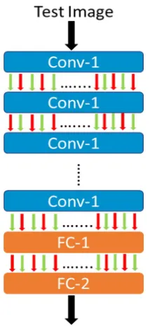
Figure 3.1 Illustration of how weight damage (red) is introduced into the network architecture.
The first step of our investigation introduces faults in the network nodes by randomly
dropping weights (setting them to zero). We consider six different architectures that
have been very effective: AlexNet, VGG16, ResNet50, GoogleNet, SqueezeNet and
YOLO. The weights are taken from the pre-trained model [52] and then fine-tuned [53]
for classification in all the six networks. Fig. 3.1 represents the weights being dropped
at every convolution layer except for the fully connected(FC) layer. The dropping of
3.3.1.1 Dropping weights using in-built function
Keras drops the weights by invoking a dropout layer in keras.layers. This function sets
the random fraction of the weights to zero and drops the weights randomly. The
dropout layer drops particular weights for a particular iteration, but for the next
iteration, different set of random weights are dropped. This is not what out experiment
requires but instead, if a particular weight has been dropped it should remain dropped
for all iterations. Furthermore, the dropout layer in keras works only while training
but it does not work while testing, which is a big setback for the nature of our
experiments. Most of our work is while testing, as we will be observing how the
network performs while the weights have been damaged.
To overcome the above shortcomings, a permanent drop layer is used. This function
invokes the kernel of the keras by using the Lambda function, where we set the flag for
dropout during testing and the same weights are dropped for one following session of
Tensorflow as Keras is working as a frontend of Tensorflow. The permanent drop
function which invokes kernel layers in Keras for dropping.k refers to keras’s backend.
drop function ignores the parameter and considers it to have 0 while forward
propagation and backward propagation.
3.3.1.2 Dropping weights manually
Dropping weights manually refers to zeroing of weights by invoking each layer’s
parameters. For example if a network has five layers, we call each layer’s parameters
and set the weights to zero by randomly selecting the position of the weights that has
to be set to zero.
Figure 3.2 Toy example of weights (a) Represents weights before drop and (b) Represents weights after drop
which gives a random number from zero to the size of the tensor of weights. Random
function generator used here is a library in python which can be called by importing a
random class which has randomint() method with parameters lowest to the highest
number. This function puts all the values in a tuple and shuffles. The first number in
the tuple is given as the output. Then we traverse to that position of the network and
set that weight to zero which can be seen in Fig. 3.2. This step is repeated for all the
layers in the network. The percentage of dropped weights in all the layers remains the
same. For example, in a network with 2 hidden layer, we first go to the 1st convolution
layer and set 50% of weights to zero. Then we repeat the procedure on the 2nd
convolution layer where again the percentage of dropped weights is 50%.
After dropping the weights, the actual weight file needs to be updated, so we use a
function called set_weights in keras. Next we use save_weights to .h5 file which will
be re-used.
3.3.2 Resilience with faults at a single convolution layer
In this experiment, the network weights are dropped successively at each
so at each layer weights are dropped at varying degrees, from 0% to 100% as shown in
Figure 3.3. The effects of dropping weights at different layers were similar. Since the
last convolution layer which precedes the classifier is the most important, we consider
dropping only the weights in the last layer for this experiment. The procedure for
dropping weights is as described in Section 3.3.1.
Figure 3.3 Illustration of how weight damage (red) is introduced into the network architecture
Finding the fitness of weights in the network requires ranking mechanism for each
filter’s importance. There are different ranking mechanisms including [54]. In Keras
we don’t have enough liquidity in modifying the layers and hence we use Pytorch
which gives full access to each layer and allows modifications. Hence this part of the
thesis is performed in Pytorch which is built on torch framework. The ranking
mechanism used is Taylor Ranking.
3.3.3.1 Taylor Ranking
Taylor Ranking criteria does pointwise multiplication of activation in each batch with
its gradient, where activations are the output features from the convolution layer. The
same process is repeated for all the activations in that convolutional layer. Then we
sum all the dimensions except for the dimension of the output. This will give the rank
of each filter in the network and it can be dropped by zeroing the weights [55].
𝑣𝑎𝑙𝑢𝑒 = + 𝐹) 𝑔)
),- ………... (3.1)
In Equation (3.1) value gives the point wise multiplication of activation (F) and the
gradient (g) which is then summed to the batch size i.e. value will have a dimension of
(batch_size) x (dim(filter)) x (number of filter). By normalizing in the direction of the
filter we will have a rank filter of dimension 1 x (number of filter) as can be seen in
Equation (3.2).
For example in VGG16 batch size is 32, output from the activations has a dimension of
256 and the spatial dimension of the network is 112x112 and hence the dimension of
the gradient will be 32x256x112x112. When the gradient and activation gets, pointwise
multiplied and normalized (averaging) with the dimension of the filter, the output will
be a vector with ranks of size 256, each corresponding to a filter.
3.4 Self-Healing by Re-training
In this Section we explore whether partially damaged DCNNs have the ability to
self-heal and recover their performance by retraining. We address this question in two
steps. First, we retrain the network on the entire dataset using Resilient propagation
(Rprop). Rprop is a learning heuristic for supervised learning in feedforward artificial
neural networks, where the learning rate is adapted for each of the parameters. The
combined with dropout. Thus, we expect that it will work well when the network is
subjected to faults because this resembles dropout. Furthermore, Rprop is faster than
standard gradient descent back-propagation. This increase in training speed can be
used for efficient retraining. Retraining was done using Keras with tensorflow at the
background. After the weights were dropped at each stage, the network with Rprop as
the optimizer to obtain the testing accuracy. While retraining, we carefully inspected
the dropped weights to make sure they don't change. We used a permanent drop by
calling the core layers of keras. A permanent drop is meant to drop weights during
training and testing. There are different methods through which the network is
re-trained.
3.4.1 Re-training with AdaGrad
AdaGrad [56] or adaptive gradient allows the learning rate to adjust dependent on
parameters. It performs bigger updates for rare parameters and little updates for
continuous one. Because of this, it is appropriate for sparse data, for example Natural
Language Processing. Another favorable attribute is that it fundamentally disposes of
the need to tune the learning rate. Every parameter has its own learning rate that is
learning rate is very small to the point that the framework quits learning [57]. The
equation is shown below.
𝑤
)>-= 𝑤
)−
@AB CDB CDE
∗ 𝑔
G………. (3.3)
𝑔
G= ∇𝐽(𝑤
))
……….. (3.4)
In Equation (3.3) 𝑤)>- and 𝑤) refers to the parameters at time step i+1 and i
respectively. In the Equation (3.4), degradation of learning rate increases with every
iteration. ∇𝐽 𝑤G is the objective function which we are trying to reduce. This method
would take too long to train as it keeps adding all the past gradients to reduce the
learning rate. There comes a point where the learning rate is so low that the parameters
stop learning.
3.4.2 Re-training with Adadelta
AdaDelta [58] is an expansion of AdaGrad that tries to lessen the forceful,
discarding the past squared gradients it recursively calculates the decaying average of
the past squared gradients [57].
w
K>-= 𝑤
)−
LMN ∇O BPELMN AQ B
∗ 𝑔
G……….. (3.5)
𝑅𝑀𝑆 𝑔
U G= 𝐸 𝑔
U+ ∈
……….. (3.6)
𝑅𝑀𝑆 ∇𝜃
U G= 𝐸[∇𝜃
U]+ ∈
……...……….. (3.7)
Where RMS refers to root mean squares, 𝐸 𝑔U is the decaying average over past
squared gradients. 𝐸[∇𝜃] is the decaying average of the squared parameters. ∈ is the
smoothing term to avoid division by zero. From the above equation, instead of keeping
the information from all the past gradients but only keeps the past squared gradients.
3.4.3 Re-training with Rprop
Rprop [59] refers to resilient back propagation and is a local adaptive learning scheme,
performing local batch training with multi layered neural network. The fundamental
princinple of Rprop is to remove the impact of size of the derivative in each weight
weight updates. This process requires no parameter tuning. The learning and
adaptation are only affected by the sign of the partial derivative. Learning is equally
spread over the network [59].
∆w
]=
+∆v
]
, if dθ > 0
−∆v
], if dθ > 0
0 , if dθ = 0
……… (3.8)
The above equation is the updating rule for Rprop where ∆𝑣G refers to the Momentum
and d𝜃denotes the sum of gradient in a particular batch. This is a method that helps
accelerate SGD in the relevant direction.
3.4.4 Re-training with ADAM optimizer
Adaptive Moment Estimation (ADAM) [60] is another technique that registers adaptive
learning rates for every parameter. This method includes decaying average of past
squared gradients like Adadelta and RMSprop, but also includes decaying average of
running down a slant, ADAM acts like a substantial ball with friction, which along
these lines inclines toward level minima in the rough surface [57].
𝑚
G= 𝛽
-+ 1 − 𝛽
-∗ 𝑔
G………. (3.9)
𝑣
G= 𝛽
U+ 1 − 𝛽
U∗ 𝑔
G……… (3.10)
∆𝑚
G=
eB-fgE
...………... (3.11)
∆𝑣
G=
hB-fgQ
…...……… (3.12)
𝑤
G>-= 𝑤
G−
@∆hB>∈
∗ ∆𝑚
G…..……….. (3.13)
Where 𝑚G refers to past squared gradient and 𝑣Gis the decaying average of the past. 𝛽
-and 𝛽U refers to decay rates. The authors propose default values of 0.9 for β1, 0.999
for β2, and 10fi for ϵ. The authors show that ADAM optimizer works best for all the
training mechanism. ADAM optimizer has been the most used optimization algorithm
for gradient descent.
We prepare ARprop, that combines two well used optimizing algorithms, ADAM and
Rprop. The best feature of Rprop is the way it updates the weights using Manhattan
Rule [42] that makes it faster than any other optimizing algorithm including ADAM
optimizer. We use ADAM optimizer’s learning rate decay method and update the
weight using Manhattan rule by keeping the momentum of the gradients. So the
equation used is:
∆w
]=
+∆p
]
, if dθ > 0
−∆p
], if dθ > 0
0 , if dθ = 0
……… (3.14)
Where p is ADAM’s learning rate decaying method.
𝐩 =
𝛈∆𝐯𝐭>∈
∗ ∆𝐦
𝐭……… (3.15)
The other method that was tried was using AdaGrad with Rprop which makes it faster
but after a certain decay of learning rate, the network stops learning and results are not
Figure 3.4 Network Pruning flow diagram
3.5 Pruning
Pruning refers to deleting or eliminating the parts of the network without sacrificing
performance. This is done by reducing the size of the parameters by eliminating the
weights i.e. dropping the weights. In our example, we follow a procedure to prune
VGG16 and GoogleNet architecture to the size of SqueezeNet by using manual drop of
weights without considering the fitness of the weights. The flow diagram of this
In Fig. 3.4 we follow the same procedure as described in this chapter. The network is
transfer learned for MSCOCO dataset. Then the network goes though the dropping of
weights, as SqueezeNet consists of 1.2M parameters VGG16 must be reduced from 7M
parameters to 1.2M and hence, resulting in 82% reduction in the number of its
parameters. Similarly GoogleNet has 5.6M parameter so it is reduced by 78% to reach
the size of SqueezeNet.
Next step is retraining the healthy part of the network. The ADAM optimizer, because
of its exponential decay and momentum decay, gives the best result for retraing after
50% of weights have been dropped but it takes considerably more time than its
competitors.
Advantages of pruning a network includes less computational capacity required while
testing or predicting, hence the results can be faster. Memory usage is reduced thus
pruning can be good for computational time and space. Disadvantage of pruning the
Chapter 4
Results
This chapter describes how the each of CNN’s acts when subjected to failure followed
by how fast each of these networks can heal itself with training. This chapter also has
results of pruning VGG16 and GoogleNet.
4.1 Resiliency with faults across the network
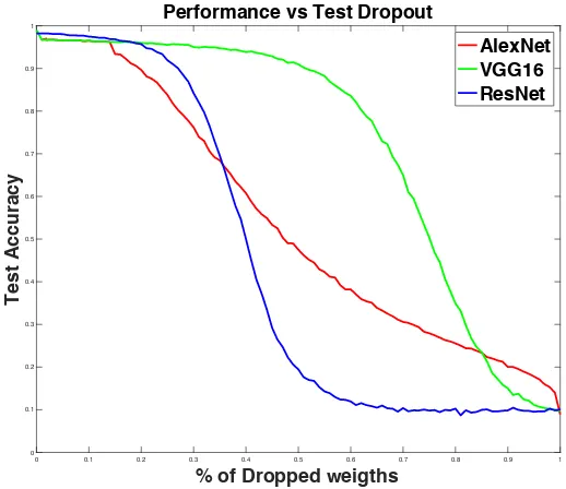
Figure 4.1 shows the result of test accuracies after the weights have been dropped for
to 100%. Our results indicate that AlexNet is the least resilient of the three networks as
it only has five layers and fewer parameters compared to the others. At just 20% of
dropped weights the test accuracy reduces to 40%. On the other hand, VGG16 is the
most resilient. With almost 50% of the weights dropped the network still maintains
accuracy close to 80%. For ResNet50 the accuracy falls suddenly when approximately
30% of weights are dropped.
Figure 4.1 Accuracy vs Percent of Dropped Weights across the full network in AlexNet, VGG16 and ResNet
Even though ResNet has more layers when compared to VGG16, it is less resilient. This
0 0.1 0.2 0.3 0.4 0.5 0.6 0.7 0.8 0.9 1
% of Dropped weigths
0 0.1 0.2 0.3 0.4 0.5 0.6 0.7 0.8 0.9 1
Test Accuracy
Performance vs Test Dropout
we explored the effects of filter size and found that networks with smaller filter size are
more resilient.
ResNet was introduced to tackle the problem of redundancy in deep convolutional
neural network by using residual blocks or skip connections. This reduces the
redundancy in the network. The network is found to be resilient when its weights are
dropped. ResNet, with the help of residual blocks, already drops or skips parameters
that can be considered as unimportant or redundant. For this reason ResNet remains
less resilient when compared to VGG16, even though ResNet has more number of
parameters.
Each of these experiments have been run 3 times and all the results were similar. So, all
these experiments are performed for the fourth time and results were noted down and
plotted as a graph. For the cases of 50% and 25% of faults the experiments are
performed for 6 times and then the results have been averaged out.
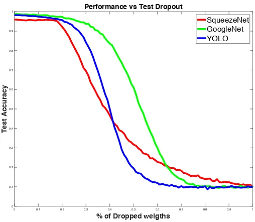
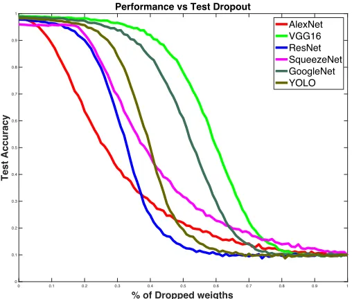
Fig. 4.2, shows the results of performance after the weights have been dropped in
SqueezeNet, GoogleNet and YOLO. The percent of weights dropped was varied from
0% to 100%. Our results indicate that SqueezeNet is the least resilient of the three
size to 1x1 instead of 3x3 filters and it has fewer parameters compared to the other
[image:65.612.179.433.172.393.2]network.
Figure 4.2 Accuracy vs Percent of Dropped Weights across the full network in SqueezeNet, GoogleNet and YOLO.
At just 30% of dropped weights the test accuracy reduces to 40%. On the other hand,
GoogleNet is the most resilient network because it has the most number of parameters
which excludes residual blocks and containing of redundant layers.
YOLO is a very popular convolutional neural network. Because of residual block in the
network it faces the same problem as ResNet and starts to show decline in performance
0 0.1 0.2 0.3 0.4 0.5 0.6 0.7 0.8 0.9 1
% of Dropped weigths
0 0.1 0.2 0.3 0.4 0.5 0.6 0.7 0.8 0.9 1
Test Accuracy
Performance vs Test Dropout
GoogleNet on the other hand is the most resilient out of YOLO and ResNet because of
more trainable parameters and does not include residual blocks similar to VGG16
[image:66.612.178.434.201.423.2]model.
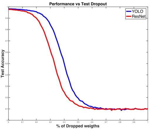
Figure 4.3 Accuracy vs Percentage of dropped weights across the full network comparing ResNet and YOLO
Fig. 4.3 shows the comparison of two similar networks i.e. ResNet and YOLO as both
have residual blocks which means it may not redundant layers which we were trying
to remove from the network, But, because YOLO has more parameters compared to
ResNet and the residual blocks are only for 2 convolution layer as described in Chapter
2. Yolo performs better than ResNet.
0 0.1 0.2 0.3 0.4 0.5 0.6 0.7 0.8 0.9 1
% of Dropped weigths
0 0.1 0.2 0.3 0.4 0.5 0.6 0.7 0.8 0.9 1
Test Accuracy
Performance vs Test Dropout
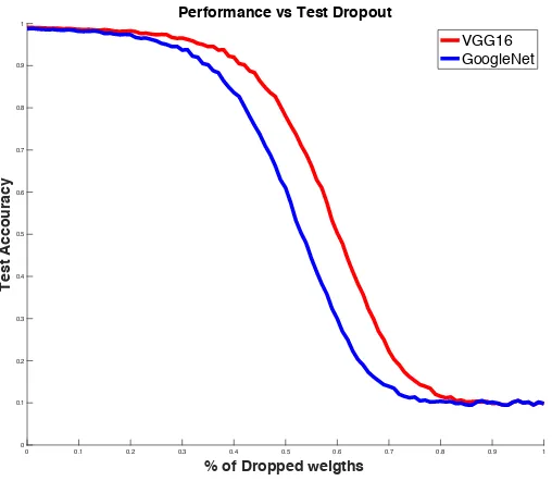
Figure 4.4 ccuracy vs Percentage of dropped weights across the full network comparing VGG16 and GoogleNet
Fig. 4.4 shows the comparison of VGG16 vs GoogleNet architecture in terms of
resiliency. VGG16 architecture does slightly better compared to GoogleNet which has
almost 10 times the parameters of GoogleNet. Hence 60% drop of weights in these
networks would leave GoogleNet almost with 1 million parameters but the VGG16 still
will be having 60 million parameters.
Fig. 4.4 shows that VGG16 remains as the most resilient of all the architectures and
AlexNet is the least resilient architecture. GoogleNet comes second to VGG16 as can be
0 0.1 0.2 0.3 0.4 0.5 0.6 0.7 0.8 0.9 1
% of Dropped weigths
0 0.1 0.2 0.3 0.4 0.5 0.6 0.7 0.8 0.9 1
Test Accouracy
Performance vs Test Dropout
Figure 4.5 Accuracy vs Percentage of dropped weights across the full network for all the architecture
[image:68.612.180.434.116.332.2]4.2 Resilience with faults at a single convolution layer
Fig. 4.6 shows the performance of AlexNet, VGG16 and ResNet when weights have
been dropped. AlexNet has a gradual drop in accuracy, whereas VGG16 does well until
60% of weights are dropped and has a sudden drop in accuracy after that. ResNet's last
layer acts the same way as it did when the weights were dropped throughout the
network. Our experiments illustrate that DCNNs start losing performance in a similar
manner whether faults are introduced across the entire network Fig. 4.3 or just at a
0 0.1 0.2 0.3 0.4 0.5 0.6 0.7 0.8 0.9 1
% of Dropped weigths
0 0.1 0.2 0.3 0.4 0.5 0.6 0.7 0.8 0.9 1
Test Accuracy
Performance vs Test Dropout
single layer Fig. 4.6. This result indicates that networks have a high level of inbuilt
[image:69.612.177.436.172.396.2]resilience, due to the redundant nature of DCNN architectures.
Figure 4.6 Accuracy vs Percent of Dropped Weights in last convolution layer for AlexNet (red), VGG (green), and ResNet
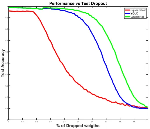
Similar experiment were performed on GoogleNet, YOLO and SqueezeNet where the
weights are dropped at varying degree from 0% to 100% from layer just before its
classifie. For SqueezeNet model the layer before the last convolutional layer is dropped
as the filter size is 1x1 this layer acts as a fully connected layer. With YOLO the last
residual block is where the errors are induced. In GoogleNet we chose the last inception
layer. Figure 4.7 shows the results for SqueezeNet, YOLO and GoogleNet when weight
0 0.1 0.2 0.3 0.4 0.5 0.6 0.7 0.8 0.9 1
% of Dropped weigths
0 0.1 0.2 0.3 0.4 0.5 0.6 0.7 0.8 0.9 1
Test Accuracy
Performance vs Test Dropout
Figure 4.7 Accuracy vs Percent of Dropped Weights in last convolution layer for SqueezeNet (red), YOLO(blue), and GoogleNet(green)
SqueezeNet has a gradual drop in accuracy, whereas GoogleNet does well until 70% of
weights are dropped and has a sudden drop in accuracy after that. The YOLO last layer
acts the same way as it did when the weights were dropped throughout the network
just like ResNet.
Our experiments illustrate that DCNNs start losing performance in a similar manner
whether faults are introduced across the entire network Fig. 4.3 or just at a single layer
Fig. 4.6. This result indicates that networks have a high level of inbuilt resilience.
0 0.1 0.2 0.3 0.4 0.5 0.6 0.7 0.8 0.9 1
% of Dropped weigths
0 0.1 0.2 0.3 0.4 0.5 0.6 0.7 0.8 0.9 1
Test Accuracy
Performance vs Test Dropout
4.3 Resilience with faults across the entire network with fitness
Figure 4.8 Accuracy vs percentage drop in AlexNet, VGG16 and ResNet with fitness
Fig. 4.8 shows the results of AlexNet, VGG16 and ResNet when weights were dropped
considering the fitness of the weights. The percent of weights dropped was varied from
0% to 100% starting from least fit to most fit based on Taylor ranking method. Our
results indicate that AlexNet gradually loses its accuracy. On the other hand, VGG16
retains its properties and gives acceptable results even after 60% of dropped weights.
0 0.1 0.2 0.3 0.4 0.5 0.6 0.7 0.8 0.9 1
% of Dropped weigths
0 0.1 0.2 0.3 0.4 0.5 0.6 0.7 0.8 0.9 1
Test Accuracy
Performance vs Test Dropout
Fig. 4.8. ResNet starts losing accuracy at 35% of dropped weights, seen previously
[image:72.612.186.443.202.424.2]because of its residual blocks.
Figure 4.9 Accuracy vs percentage drop in SqueezeNet, GoogleNet and YOLO with fitness
Fig. 4.8 shows the results of SqueezeNet, GoogleNet and YOLO when weights were
dropped considering the fitness of the weights. The percent of weights dropped was
varied from 0% to 100% starting from least fit to most fit. Our results indicate that
SqueezeNet gradually looses its accuracy as it is the smallest network of all, while
YOLO just like ResNet remains the same as in Section 4.2 because of the residual block.
On the other hand, GoogleNet retains its properties and gives acceptable results even
0 0.1 0.2 0.3 0.4 0.5 0.6 0.7 0.8 0.9 1
% of Dropped weigths
0 0.1 0.2 0.3 0.4 0.5 0.6 0.7 0.8 0.9 1
Test Accuracy
Performance vs Test Dropout
after 50% of dropped weights, as can be seen in Fig. 4.9, as it has large number of
parameters and hence it shows it can be pruned well to match the size of the other
network.
4.4 Network Self-Healing by Retraining
We retrained each of the three networks after introducing faults ranging from 0% to
100% across the entire DCNN. In all cases, we found significant recovery of accuracy
after retraining. This type of retraining is a form of self-healing that utilizes the
surviving connections after parts of the network have been damaged.
4.4.1 Retraining with AdaGrad Optimizer
All the three networks AlexNet, VGG16 and ResNet show significant improvement
after retraining seen in the Fig. 4.10. Even though VGG16 does well while the weights
have been dropped in Fig. 4.5, ResNet does remarkably well while re-training mainly
because of residual layers or skip connections, The ResNet network, which had skipped
re-Figure 4.10 Performance recovery by retraining (self-healing) after weights are dropped throughout the AlexNet, VGG16, ResNet network.
Fig. 4.11 shows that retraining improves in the next three architecture, out of which
YOLO performs remarkably well compared to GoogleNet and SqueezeNet up until
60% of the weights have been corrupted. This is because of the residual layer present
in the architecture. After 60% of dropped weights the network suddenly shows a
significant drop in the accuracy as can be seen in the
![Figure 2.5 ResNet Architecture [42]](https://thumb-us.123doks.com/thumbv2/123dok_us/32809.2591/30.612.248.365.103.638/figure-resnet-architecture.webp)