rsos.royalsocietypublishing.org
Research
Cite this article:Grimes DR, Fletcher AG, Partridge M. 2014 Oxygen consumption dynamics in steady-state tumour models.
R. Soc. open sci.1: 140080.
http://dx.doi.org/10.1098/rsos.140080
Received: 3 June 2014 Accepted: 30 July 2014
Subject Areas:
biophysics/medical physics/radiation biophysics
Keywords:
mathematical modelling, hypoxia, oxygen
Author for correspondence:
David Robert Grimes
e-mail: davidrobert.grimes@oncology.ox.ac.uk
Electronic supplementary material is available at http://dx.doi.org/10.1098/rsos.140080 or via http://rsos.royalsocietypublishing.org.
Oxygen consumption
dynamics in steady-state
tumour models
David Robert Grimes
1
, Alexander G. Fletcher
2
and
Mike Partridge
1
1Cancer Research UK/MRC Oxford Institute for Radiation Oncology, Gray Laboratory,
University of Oxford, Old Road Campus Research Building, Off Roosevelt Drive, Oxford OX3 7DQ, UK
2Wolfson Centre for Mathematical Biology, Mathematical Institute, University of
Oxford, Andrew Wiles Building, Radcliffe Observatory Quarter, Woodstock Road, Oxford OX2 6GG, UK
1. Summary
Oxygen levels in cancerous tissue can have a significant effect on treatment response: hypoxic tissue is both more radioresistant and more chemoresistant than well-oxygenated tissue. While recent advances in medical imaging have facilitated real-time observation of macroscopic oxygenation, the underlying physics limits the resolution to the millimetre domain, whereas oxygen tension varies over a micrometre scale. If the distribution of oxygen in the tumour micro-environment can be accurately estimated, then the effect of potential dose escalation to these hypoxic regions could be better modelled, allowing more realistic simulation of biologically adaptive treatments. Reaction–diffusion models are commonly used for modelling oxygen dynamics, with a variety of functional forms assumed for the dependence of oxygen consumption rate (OCR) on cellular status and local oxygen availability. In this work, we examine reaction– diffusion models of oxygen consumption in spherically and cylindrically symmetric geometries. We consider two different descriptions of oxygen consumption: one in which the rate of consumption is constant and one in which it varies with oxygen tension in a hyperbolic manner. In each case, we derive analytic approximations to the steady-state oxygen distribution, which are shown to closely match the numerical solutions of the equations and accurately predict the extent to which oxygen can diffuse. The derived expressions relate the limit to which oxygen can diffuse into a tissue to the OCR of that tissue. We also demonstrate that differences between these functional forms are likely to be negligible within the range of literature estimates of the hyperbolic oxygen constant, suggesting that the constant consumption rate approximation suffices for modelling oxygen dynamics for most values of OCR. These approximations also allow the rapid identification of situations where hyperbolic
2
rsos
.ro
yalsociet
ypublishing
.or
g
R.
Soc
.open
sc
i.
1
:1
40080
...
consumption forms can result in significant differences from constant consumption rate models, and so can reduce the computational workload associated with numerical solutions, by estimating both the oxygen diffusion distances and resultant oxygen profile. Such analysis may be useful for parameter fitting in large imaging datasets and histological sections, and allows easy quantification of projected differences between functional forms of OCR.
2. Introduction
It has been known since the pioneering work of Gray and co-workers in the 1950s [1] that well-oxygenated tissue responds better to radiotherapy and chemotherapy than by up to a factor of 3 relative to tumours with extensive hypoxia. This relative boosting effect of oxygen on cell-kill is often quantified by the oxygen enhancement ratio (OER), which is of fundamental importance in radiotherapy [2]. The prognostic influence of hypoxia has led to the concept of dose painting [3,4] in radiotherapy, which proposes that hypoxic regions of a tumour could be given an increased dose to mitigate their inherent radioresistance. Imaging modalities such as positron emission tomography (PET) can be coupled with hypoxia binding tracers such as 18F-fluoromisonidazole to allow the non-invasive estimation of hypoxia in vivo[3]. Although this approach is promising, the spatial resolution remains prohibitively low [5], as PET imaging is physically constrained to a millimetre-scale resolution, while oxygen tension is known to vary significantly over tens of micrometres [6–9], owing to the relatively short oxygen diffusion distances in tissue.
To maximize the potential advantages of a dose painting approach to treatment outcome, it is vital that the underlying oxygen distributions are well understood. Mathematical modelling of oxygen transport at micrometre scales is therefore required to estimate oxygen distributions. In continuum formulations, oxygen is assumed to diffuse through tissue while simultaneously being consumed by the respiring cells. Models of this type have been developed for spherical geometries to describe the oxygen tension in multicellular tumour spheroid (MCTS) growth [10–12] and cylindrical geometries for blood vessel perfusion modelling [8,9,13,14]. This approach has been widely used in various tissue geometries and situations [8–11,15–20] to estimate the oxygen dynamics through a tissue. Several functional forms of the oxygen consumption rate (OCR) have been proposed. In some formulations, it is treated as a constant [8,9] while elsewhere the OCR is assumed to vary with oxygen tension, typically obeying a rectangular hyperbolic relationship, similar in form to Michaelis–Menten kinetics or the Langmuir adsorption isotherm. This particular functional form has been shown to be a good approximation in a variety of tissues, both healthy and cancerous [21–24]. A typical hyperbolic reaction rate is given by
νmaxs
s+Km, (2.1)
wheresis the substrate concentration,νmaxis the maximum reaction rate andKmis substrate level where νis halfνmax.
For cellular oxygen consumption, this model is phenomenological, and its sigmoidal form is intended to capture the observation that the OCR in a given tissue is typically lower under hypoxic conditions than under normoxia. From a biological perspective, such dynamics may be explained by the observation that under hypoxic conditions, expression of proteins such as HIF-1 can lead to downregulation of mitochondrial oxygen consumption, as well as affecting cell cycling [25]. The nonlinear form of (2.1) renders reaction–diffusion equations involving hyperbolic kinetics analytically intractable in general, and so they must be solved numerically.
The form of equation (2.1) suggests that the relative magnitude of the constant Km for oxygen
has a distinct effect on the shape of the consumption rate curve. The literature to date indicates that this constant for oxygen is quite low compared with typical oxygen tension in a vessel, typically Km1 mm Hg [26–28]. This may suggest only small predicted differences between the two consumption
3
rsos
.ro
yalsociet
ypublishing
.or
g
R.
Soc
.open
sc
i.
1
:1
40080
...
availability, allowing oxygen to diffuse deeper into the respiring tissue than in the constant case. Thus, if all other parameters are kept the same, the oxygen diffusion distance in the hyperbolic model will be always greater than for the constant consumption rate case. Under what circumstances this difference may be significant in a given situation is an open question, and part of the motivation for this work.
Previous literature has outlined how oxygen diffusion distance can be analytically derived for the constant consumption rate case in the case of cylindrical [8] and spherical [10] geometries, and to date numerical approaches have been used when considering non-constant kinetics, owing to the analytic intractability of the problem [29]. The significant drawback of such approaches is that the diffusion boundaries must be specified by the user, rendering the process uncertain and making direct comparison between constant oxygen consumption models and hyperbolic kinetic models difficult. Despite the small literature estimates ofKmfor oxygen, there may be cases where significant differences emerge between
constant consumption and M–M case. It would be beneficial to have a simple method of quantifying the effects of both constant OCR and hyperbolic consumption rate forms, and a specifically a method for estimating the predicted oxygen diffusion distance in the hyperbolic case explicitly. Such a method would also have to be capable of explicitly relating OCR to the oxygen diffusion distance. In this work, we derive analytical approximations for hyperbolic-type models in both spherical and cylindrical geometry, and contrast these to constant consumption models. We show how oxygen diffusion distance is governed by OCR, and we show how the models derived can be used to obtain a value for the oxygen diffusion distance and rapid estimation of the expected oxygen profile. As the oxygen tension and associated boundaries can be estimated analytically, this can reduce computational workload when modelling systems of such elements or performing image analysis on vessel sections. We present results of this analysis for key quantities of interest such as expected diffusion distance and oxygen distribution and discuss the implications for oxygen modelling at a micrometre scale.
3. Methods and models
3.1. Spherical symmetry
We adopt a continuum modelling approach, deriving a reaction–diffusion equation governing the spatio-temporal dynamics of oxygen in an avascular tissue. Adopting spherical polar coordinates, we suppose that the centre of the MCTS is located atr=0. Since the average doubling time of cells in an MCTS is much longer than the typical time scale of oxygen diffusion across the spheroid, we make the simplifying assumption that the spheroid radius, denoted byro, is constant over the time scale of measurement.
We initially suppose that the spheroid is sufficiently large that a central anoxic region exists where the oxygen concentration is zero. We denote the radius of this anoxic region byrn, so that oxygen partial
pressure is zero in the region 0≤r≤rn, andrnis the boundary to which oxygen can penetrate fromro.
For convenience, we letrc=ro−rndenote the width of the viable rim of the tissue. We further assume
the MTCS is suspended in a well-mixed growth medium [10,30].
We assume that spherical symmetry is preserved, as illustrated infigure 1, and we letp(r,t) denote the partial pressure of oxygen at a distancerfrom the centre of the MCTS at timet. We consider changes in oxygen partial pressure due to two processes: Fickian diffusion into and within the MCTS, and cellular consumption. We also make the simplifying assumption that the diffusion coefficient of oxygen, denoted byD, is spatially invariant. We leta(p) denote the rate of cellular consumption of oxygen, which may depend on the local oxygen partial pressure. It can readily be shown that for typical literature values of the oxygen diffusion constantD that oxygen diffusion through an MCTS occurs on a time scale of seconds and a steady-state approximation is therefore acceptable, under whichpsatisfies the reaction–diffusion equation
0=D r2
d dr
r2dp dr
−Ωa(p) (3.1)
in the regionrn<r<ro, whereΩ=3.0318×107mm Hg kg m−3arises from Henry’s law as outlined in
previous work [10]. Although one could readily define a constant that subsumesa(p) andΩ, we will keep them separate in this work to reflect their physical meaning—specificallya(p) is the oxygen consumption rate in SI units of volume of oxygen per unit mass per unit time. If the two terms are subsumed into a resultant termΩa(p), then this yields consumption in units of oxygen partial pressure per unit time. To close this system, we must impose appropriate boundary conditions. We impose the regularity condition p(rn)=0 at the anoxic edge and assume that the exterior medium is well mixed and that oxygen is in
4
rsos
.ro
yalsociet
ypublishing
.or
g
R.
Soc
.open
sc
i.
1
:1
[image:4.522.110.417.44.183.2]40080
...
(a)
100 µm
O2in ro
rn rc
(b)
Figure 1.(a) Spherical geometry: a cross section of a tumour spheroid of radiusro. Oxygen partial pressure atroispoand oxygen partial
pressure falls to 0 atrn, the radius of the anoxic region. (b) A cross section of a DLD-1 colorectal spheroid with same regions visible [10].
the Dirichlet boundary conditionp(ro)=po. It is important to note thatrn, the anoxic radius, is not known a prioribut can be derived from first principles, as outlined below.
3.1.1. Constant consumption rate
If the OCR is taken to be constant then it is possible to derive a closed-form analytic solution to the model [10]. In this case, oxygen consumption is a constant so thata(p)=ao. The exact solution is given
analytically by
p(r)=po+ aoΩ
6D
r2−r2o+2r3n
1 r −
1 ro
=aoΩ
6D
r2+ 2r
3
n r −3r
2
n
(3.2)
forrn≤r≤ro. It can further be shown [10] that the maximum radius that oxygen can penetrate before
the formation of an anoxic core is given by
rl=
6Dpo
Ωao. (3.3)
It is important to note thatrnis not knowna prioriand needs to be calculated. In equation (3.2), the anoxic
radiusrnis undetermined and can be explicitly calculated [10] to give
rn=ro
1 2−cos
arccos(1−2r2
l/r2o)−2π
3
. (3.4)
For spheroids sufficiently small to have no central anoxia,rn=0 and a similar analysis can be performed.
3.1.2. Hyperbolic consumption rate
In the hyperbolic case, there is no exact analytical solution to equation (3.1). The general approach taken in the literature has been to use numerical methods to estimate the local partial pressure [11]. A drawback of this approach is the lack of a closed-form expression for the boundary of the anoxic radius,rn. This differs from that in the constant model, as the reduced OCR in the hyperbolic formulation
yields a longer diffusion distance. Denoting this modified anoxic radial distance byr∗n, we can establish a phenomenological approximation which captures the behaviour of the function and satisfies the conditions thata(p)=0 at the anoxic edgernwith a maximum value fora(p) atro. Close to the interface
between oxygenated and hypoxic regions, the oxygen curve falls to zero with a zero gradient, which can be readily approximated by a quadratic parabola-like fit. If we defineaoas the maximum OCR, then a
suitable approximation fora(p) is given by
a(p)= aop(r) p(r)+Km ≈
ao(r−r∗n)2
(r−r∗n)2+kr, (3.5)
where
kr=(ro−r∗n)2 Km
5
rsos
.ro
yalsociet
ypublishing
.or
g
R.
Soc
.open
sc
i.
1
:1
[image:5.522.146.368.45.255.2]40080
...
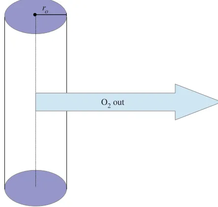
O2 out
ro
Figure 2.Schematic diagram of a Krogh-type vessel model in cylindrical geometry, with vessel radiusro.
Substituting (3.5) into (3.1) with the same boundary conditions as the constant consumption rate case, p(r∗n)=0 andp(r∗n)=0, we obtain the analytic solution
p(r)=aoΩ 6D
r2−3r∗n2+2r ∗
n3−6krr∗n
r +6kr−3
krπr∗n+6
krr∗narctan
√
kr r−r∗n
+ (6 √
krr∗n2−6kr3/2) arctan ((r−r∗n)/
√
kr)
r +
6krr∗n r −3kr
ln
(r−r∗n)2+kr kr
. (3.7)
To estimate r∗n in this case, (3.8) is solved subject to p(ro)=po. From this, r∗n can be found to any
required degree of precision from the resulting expression, allowing determination of this boundary. It is important to note that oxygen can diffuse further in the hyperbolic formulation, and subsequently the anoxic region is decreased relative to the constant consumption case so thatr∗n≤rn. In the case of
spheroids sufficiently small to have no central anoxia,r∗n=0.
3.2. Cylindrical symmetry
Cylindrically symmetric reaction–diffusion equations are often encountered in Krogh-type models to simulate oxygen flow from a blood vessel [8,9,13] under the reasonable assumption that vessels secrete oxygen perpendicular to their walls. In these situations, they present a reasonable approximation of a length of blood vessel running through a tumour. Such a situation is illustrated infigure 2. In this case, the steady-state oxygen distribution satisfies
0=D r
d dr
rdp dr
−a(p)Ω (3.8)
for all 0≤r≤rc, wherercis the diffusion limit from the vessel.
3.2.1. Constant consumption rate
With a constant consumption rate,ao, an exact solution is possible. For a vessel of radiusrowith boundary
conditionsp(rc)=p(rc)=0 andp(ro)=po, the solution to (3.8) is given by
p(r)=po+ aoΩ
4D
r2−r2o−2r2cln r ro
. (3.9)
Unlike the spherically symmetric case, there is no corresponding analytical expression for the diffusion distancerc but this can be readily estimated using root-finding methods when equation (3.9) is equal
6
rsos
.ro
yalsociet
ypublishing
.or
g
R.
Soc
.open
sc
i.
1
:1
40080
...
3.2.2. Hyperbolic consumption rate
Analysis analogous to the spherical geometry can be applied in the hyperbolic case, with the caveat that the substitution term is modified, as in this case diffusion is out from the vessel and must be zero at the radiusr∗c. In this case, oxygen should diffuse further from the vessel than in the constant consumption rate case. This approximation is given by
a(p)= aop(r) p(r)+Km
ao(r∗c−r)2
(r∗c −r)2+lr, (3.10)
where
lr=(r∗c−ro)2Km
po. (3.11)
Solving (3.8) subject to the boundary conditionsp(r∗c)=p(rc∗)=0 andp(ro)=poyields an expression that
is analytically tractable, but unwieldy. The first derivative of the solution is given by
p(r)=aoΩ 2D
r+2r∗c
√
lrarctan ((r∗c−r)/
√
lr)−lrln((r∗c−r)2/lr)−r∗c2 r
. (3.12)
To findr∗c, the modified diffusion distance, equation (3.12) is integrated with respect torsubject top(r∗c)= 0. Equation (3.12) can be solved analytically, producing a long expression which is not shown here for the sake of brevity. The full solution and code is supplied in the electronic supplementary material for reference. The resulting form is then evaluated with conditionp(ro)=poso thatr∗c may be found to any
desired degree of accuracy.
3.3. Simulations and comparison with numerical solutions
In both geometries, the oxygen distributions resulting from both models were simulated with the maximum consumption rate parameter a varying over an order of magnitude so that 2.5×10⁻⁷≤
a≤1.5×10⁻⁶m3kg−1s−1, corresponding to the range 7.50–45.45 mm Hg O2s−1. For the spherical geometry, the external partial pressure was taken as 100 mm Hg. In the cylindrical geometry, both ‘arterial’ (100 mm Hg) and ‘venous’ (40 mm Hg) source partial pressures were considered and vessel radius was fixed at ro=5µm. These values were chosen as illustrations of the typical case, but in
tumours chaotic vasculature often means significant variation in these values and can result in lower oxygen partial pressures [31], so for the cylindrical case a chaotic partial pressure of 20 mm Hg was also simulated. A value for the diffusion constant close to that of water (D=2×10⁻⁹m2s−1) [8,9] was also used.
For each set of simulation parameters, the oxygen tension profile and diffusion length (anoxic radius in the spherical geometry, diffusion distance in the cylindrical geometry) were compared and the differences between both models for the given parameter set computed. The analytical approximations were contrasted with the numerical solutions to gauge how well they described the underlying behaviour of these models. As the value ofKm in the literature is typically≤1 mm Hg [24,26], a value
of 1 mm Hg was used in these simulations. To examine the sensitivity of the model to this parameter, simulations using values of 0 mm Hg≤Km≤10 mm Hg were examined.
4. Results
4.1. Validity of the analytical approximation
7
rsos
.ro
yalsociet
ypublishing
.or
g
R.
Soc
.open
sc
i.
1
:1
[image:7.522.152.371.453.620.2]40080
...
280 300 320 340 360 380 400 420 440 460 480 500
0 20 40 60 80 100
distance from spheroid centre (mm)
partial pressure (mm
Hg)
(a)
(b) (c)
0 20 40 60 80 100 120
20 40 60 80 100
distance from vessel centre (mm) distance from vessel centre (mm)
partial pressure (mm
Hg)
20 40 60 80
0 10 20 30 40
partial pressure (mm
Hg)
Figure 3.Comparisons of the approximation solution (solid line) with numerical solution (dashed line) for (a) a 500µm spheroid
(r∗n=281.62µm andpo=100 mm Hg), (b) a vessel of radiusro=5µm (r∗c =113.12µm,po=100 mm Hg, typical arterial pressure)
and (c) a vessel of radiusro=5µm (rc∗=81.36µm,po=40 mm Hg, typical venous pressure). For examples here,a=5×
10−7m3kg−1s−1andD=2×10⁻⁹m2s−1.
20 40 60 80 100
0 0.2 0.4 0.6 0.8 1.0
partial pressure (mm Hg)
ao
fraction
Figure 4.Comparison of the variation of relative oxygen consumption with oxygen partial pressure for the hyperbolic (dashed line) form
(P/(P+Km)) and the approximation (solid line) derived in this work, outlined in equation (3.5).
8
rsos
.ro
yalsociet
ypublishing
.or
g
R.
Soc
.open
sc
i.
1
:1
[image:8.522.61.470.73.385.2]40080
...
Table 1.Comparison of anoxic radii (rnandr∗n) and average difference in oxygen partial pressure (¯p) for constant and hyperbolic
consumption rate models in spherical geometry.
a(m3kg−1
s−1) r
o(µm) rn(µm) rn∗(µm) rn(µm) ¯p(mm Hg)
2.5×10⁻⁷ 500 204 153 51 0.85±0.86
. . . .
750 487 445 42 0.42±0.65
. . . .
1000 747 708 40 0.29±0.55
. . . .
5×10⁻⁷ 500 312 282 30 0.46±0.67
. . . .
750 572 545 28 0.27±0.53
. . . .
1000 827 800 27 0.19±0.45
. . . .
7.5×10⁻⁷ 500 351 328 23 0.35±0.60
. . . .
750 608 586 22 0.21±0.47
. . . .
1000 860 839 22 0.15±0.40
. . . .
1×10⁻⁶ 500 374 354 20 0.29±0.55
. . . .
750 628 609 19 0.17±0.43
. . . .
1000 880 861 19 0.13±0.37
. . . .
1.25×10⁻⁶ 500 388 371 17 0.25±0.51
. . . .
750 642 625 17 0.15±0.41
. . . .
1000 893 877 17 0.11±0.35
. . . .
1.5×10⁻⁶ 500 399 383 16 0.22±0.49
. . . .
750 652 636 15 0.14±0.39
. . . .
1000 903 888 15 0.10±0.33
. . . .
consistent. This indicates that the analytical approximation describes the function behaviour well in both geometries.
4.2. Comparison of constant and hyperbolic consumption rate models
Table 1 shows the estimated difference in boundary location between both models for a spherical geometry in the domain r∗n≤r≤ro. In all cases, oxygen penetrates deeper into the spheroid in the
hyperbolic situation, with these models having a decreased anoxic radius relative to the constant consumption model. Typically, this difference,rn, is of the order of tens of micrometres as shown in
table 1. Despite the increased oxygen penetration and reduced anoxic radius in the hyperbolic model however, the oxygen profile is largely consistent between both models for spherical geometry. An example of this is illustrated infigure 5a, where the average difference between both profiles is only 0.35±0.60 mm Hg in the regionr∗n≤r≤ro. Even in the relatively small region of interestr∗n≤r≤rn, with
greatest possible differences between both models, the mean difference is only 1.01±0.61 mm Hg. When the entire spheroid (0≤ r≤ro) is considered, differences between both models are effectively negligible,
being typically<0.5 mm Hg.
Similar trends are seen in the case of a cylindrical geometry, as shown intable 2. For the typical example illustrated infigure 5b, the average difference between the two models was 2.17±1.25 mm Hg over the entire profile, and a mean difference of 0.13±0.12 mm Hg in the region rc≤r≤r∗c. For all
simulated cylindrical profiles, the difference in this region is negligible. The difference in diffusion limit rc is relatively small in this geometry at around 10µm. However, over the entire region 0≤r≤rc,
differences between the constant consumption and hyperbolic consumption rate models are more pronounced in the cylindrical geometry.
Simulations of the hyperbolic model in both geometries were run with various values of Km to
investigate what effect this had on the expected oxygen profile. WhenKm=0 mm Hg, the hyperbolic
9
rsos
.ro
yalsociet
ypublishing
.or
g
R.
Soc
.open
sc
i.
1
:1
[image:9.522.109.414.43.545.2]40080
...
250 300 350 400 450 500
0 10 20 30 40 50 60 70 80 90 100
distance from spheroid centre (mm)
partial pressure (mm
Hg)
Km= 0 mm Hg (constant consumption)
Km= 1 mm Hg
Km= 5 mm Hg
Km= 10 mm Hg
(a)
0 20 40 60 80 100 120 140
10 20 30 40 50 60 70 80 90 100
distance from radial centre (mm)
partial pressure (mm
H
g)
(b)
Figure 5.Comparing the constant and Michaelis–Menten consumption rate models for (a) spherical geometry (ro=500µm) and
(b) cylindrical geometry (ro=5µm). In both cases,D=2×10⁻⁹m2s−1anda=5×10⁻⁷m3kg−1s−1. WhenKm=0 mm Hg,
the hyperbolic model reduces to the constant consumption case. Increased values ofKmresult in longer oxygen diffusion distances and
higher overall oxygen profiles.
between the constant and hyperbolic consumption cases increases with oxygen penetrating deeper and an increased overall oxygen profile. This behaviour is shown infigure 5witha=5×10⁻⁷m3kg−1s−1. At Km=10 mm Hg, an order of magnitude above literature values, oxygen diffuses approximately
55% further through the spheroid than in the constant consumption case. In the cylindrical case at Km=10 mm Hg, the diffusion distance is 30% greater than in the constant consumption case. This
significantly changes the oxygen profile in both geometries as well as the diffusion distance with markedly different values expected for different values of Km. However, as literature values to date
10
rsos
.ro
yalsociet
ypublishing
.or
g
R.
Soc
.open
sc
i.
1
:1
[image:10.522.57.470.72.388.2]40080
...
Table 2.Comparison of diffusion-limited radii (rcandrc∗) and average difference in oxygen partial pressure (¯p) for constant and
hyperbolic consumption rate models in cylindrical geometry (ro=5µm).
po(mm Hg) a(m3kg−1s−1) rc(µm) rc∗(µm) rc(µm) ¯p(mm Hg)
100 (arterial pressure) 2.5×10⁻⁷ 137 152 15 2.11±1.17
. . . .
5×10⁻⁷ 102 113 11 2.14±1.23
. . . .
7.5×10⁻⁷ 86 95 9 2.17±1.25
. . . .
1×10⁻⁶ 77 85 8 2.18±1.27
. . . .
1.25×10⁻⁶ 70 77 7 2.18±1.30
. . . .
1.5×10⁻⁶ 65 72 6 2.19±1.30
. . . .
40 (venous pressure) 2.5×10⁻⁷ 93 109 15 1.20±0.77
. . . .
5×10⁻⁷ 70 81 11 1.31±0.80
. . . .
7.5×10⁻⁷ 60 69 9 1.32±0.82
. . . .
1×10⁻⁶ 53 61 8 1.32±0.84
. . . .
1.25×10⁻⁶ 49 56 7 1.33±0.84
. . . .
1.5×10⁻⁶ 45 52 7 1.31±0.86
. . . .
20 (chaotic pressure) 2.5×10⁻⁷ 70 86 16 0.84±0.56
. . . .
5×10⁻⁷ 53 64 11 0.89±0.58
. . . .
7.5×10⁻⁷ 45 55 10 0.89±0.59
. . . .
1×10⁻⁶ 41 49 8 0.90±0.60
. . . .
1.25×10⁻⁶ 37 45 8 0.89±0.61
. . . .
1.5×10⁻⁶ 35 42 7 0.89±0.62
. . . .
be very close to that of the constant consumption rate case. Consequently, it is unlikely that this issue would ever be a significant factor when oxygen is the substrate but may be an issue for applying these dynamics to substances other than oxygen.
5. Discussion
While the differences in oxygen profile between the constant and hyperbolic consumption rate models are relatively small, the increased oxygen diffusion distance in the hyperbolic case may have an impact when estimating the extent of the hypoxic region. In the regions of difference between the constant and hyperbolic rate models (r∗n≤rnin the spherical case andrc≤r∗c in the cylindrical case), oxygen tension
is typically extremely low (≤1 mm Hg). This may have radiobiological significance, since OER falls to unity under tensions below 2.5 mm Hg, rendering such areas of tumour more radioresistant than the adjacent well-oxygenated regions [5]. However, the oxygen profile between the two models diverges only at very low oxygen tension, where both have increased radioresistance and should as a consequence have practically identical radio-response in most situations.
In spherical geometry, the divergence between the constant and hyperbolic consumption model is generally relatively minor, as can be seen intable 1. There are however situations where this is not the case; for example, spheroids with low consumption rates and a radius of less than 500µm, such as the first entry intable 1for a spheroid with radius 500µm and OCR of 2.5×10⁻⁷m3kg−1s−1. In this case, the difference betweenrnandr∗ncan exceed 25%, and similarly parameter combinations exist that can
yield such differences between the models. Even in these cases, the oxygen profiles for both formulations are broadly similar, differing only by very small values (1 mm Hg) in the domainr∗n<r<rn. In the
spherical case, projected differences decrease markedly for higher consumption rates and larger spheroid radii. Although the model predictions between both constant and hyperbolic consumption forms tend to yield similar oxygen profiles for realistic estimates ofKm, it might be possible to use stained spheroids
11
rsos
.ro
yalsociet
ypublishing
.or
g
R.
Soc
.open
sc
i.
1
:1
40080
...
location of the stained boundary in both models, maximal at p0.8 mm Hg. In both spherical and cylindrical geometries, the projected differences are typically≈10µm, which could allow discrimination between the models if the effective average consumption rate was accurately known. Although this could, in principle, be tested on stained spheroid sections, a difficulty arises due to the fact that the projected difference in staining boundary between the constant and hyperbolic consumption models for the same maximal consumption rateais of the same order of magnitude as the uncertainties in estimating the stained boundary [10], rendering direct comparison extremely difficult. Conversely, this implies that at current experimental resolution, the differences between the two models are negligible if maximal value ofacan be accurately deduced. This suggests that the constant OCR model is a suitable model for this geometry regardless of whether the OCR is governed by hyperbolic kinetics or not.
In cylindrical geometry, differences between the constant and hyperbolic consumption rate models were small but still more pronounced than in the spherical case. It is important to note that differences between the two models in cylindrical geometry may be considerably less than that presented here as the analytical approximation systematically overestimates the oxygen profile. Hence, it follows that differences between the constant and hyperbolic consumption rate models are even less than the values reported here. More experimental data are required to investigate this further. The models derived in this work for the cylindrical geometry are Krogh-type models, which have been commonly used to model vessel oxygenation and produce results in good agreement with clinical data [6,8,9]. This approach is not by any means the sole method of estimating oxygen diffusion, and other authors have used numerical methods, including Green’s function methods [14] to solve the reaction–diffusion equations for vessel geometry. A drawback of this method is the difficulty in assigning appropriate boundary conditions [29], a difficulty which appears to some extent in all numerical approaches to oxygen modelling. One advantage of the models proposed in this work is that the boundaries for oxygen diffusion can be readily estimated, circumventing this issue and allowing the establishment of explicit relationships between the OCR and the resultant oxygen diffusion distance. In this work, the illustrative examples show the simplest case of vessels with a constant value forpoalong the length. One limitation
of the cylindrical model is that is does not take blood flow or number of erythrocytes in the capillary into account; this could have a significant effect, as the oxygen partial pressure may decrease markedly along a vessel length. If the variation rate of oxygen pressure along the vessel length can be estimated with the relevant perfusion parameters, then it should be possible to extend the simple model presented here to consider this factor.
To gauge sensitivity to the parameterKm, simulations were run from zero to an order of magnitude
above literature values (0≤Km≤10 mm Hg). Values ofKmfar above literature values greatly increased
the diffusion differences between both geometries, and increased the overall oxygen profile significantly. As Km tended to zero, hyperbolic consumption rate models in both geometries reduced to constant
consumption models. As literature values are typicallyKm≤1 mm Hg for oxygen, the effects of higher
values can likely be neglected.
Whether constant OCR or the hyperbolic approximation models are used, the effect ofaoon oxygen
diffusion distance is important and worthy of discussion. Intuitively, we might expect that higher values of maximum consumption rate ao mean that oxygen is depleted rapidly and as a consequence the
oxygen diffusion distance is diminished. The simulations in this work reiterate this in both geometries; in the spherical configuration, increasingaocorresponded to decreasing values for the viable spherical
rimrcand increased values for the hypoxic radiusrn. In cylindrical vessel-like geometry, increasingao
acted to reduce the diffusion distancerl, as illustrated infigure 6. Unlike many numerical approaches,
the relationship between ao and diffusion distance is explicitly derived in this work. This analysis
suggests that OCR has a marked effect on tumour hypoxia in both vascular and avascular situations— for the former, high values of ao would act to reduce the distance oxygen can travel in the tissue,
potentially increasing the prevalence of hypoxic regions. In the avascular case, high values ofaowould
result in increased central anoxia. While beyond the scope of this work, this aspect is worthy of further investigation.
12
rsos
.ro
yalsociet
ypublishing
.or
g
R.
Soc
.open
sc
i.
1
:1
[image:12.522.152.370.38.208.2]40080
...
0 5 10 15
200 300 400 500 600
OCR (×10−7m3kg−1s−1)
dif
fusion distance
rl
(
m
m)
Figure 6.The variation of diffusion limitrlwith OCRao, illustrated for a spheroid with constant OCR as detailed in equation (3.3).
grasped by the consideration that OCR falls with decreasing oxygen tension in such models and as a result oxygen can penetrate further at low oxygen levels than in a comparable constant consumption case. This analysis suggests that such differences are usually minor and not typically resolvable through clinical means, but also that there are situations where a measurable difference between both approaches could arise. In the formulation established in this study, the explicit relationship between maximal OCRaand the diffusion distances in all cases can be estimated from first principles, allowing rapid quantification of oxygen boundaries in all cases.
6. Conclusion
This analysis suggests that since the effectiveKm constant for oxygen consumption is so small, only
minor differences in diffusion limit (10µm) and local oxygen partial pressure (p≤1 mm Hg in spherical geometry,p2 mm Hg in cylindrical geometry) would be expected between the constant and hyperbolic consumption rate models for the typical range of literature values ofKm. There are also
cases where differences between both forms can be significant, and the forms outlined in this work allow rapid first principles estimate of the respective oxygen profiles and diffusion distance for both constant consumption rate and hyperbolic consumption rate model forms in spherical and cylindrical geometry.
In general, the simpler constant consumption form can be used in both spherical and cylindrical geometries for most situations. The models outlined also allow quick identification of situations where both models are expected to produce significantly different results, and suggestions even in these limited situations the oxygen profiles for both approaches are broadly similar. In oxygen modelling situations where hyperbolic kinetics are required, the analytical steady-state approximations outlined in this work could be used readily, allowing rapid estimation of the oxygen diffusion limit and projected oxygen profile.
Data accessibility.The full solution of equation (3.12) can be found in Mathematica Format uploaded as supplementary
material.
Funding statement.D.R.G. and M.P. are funded by Cancer Research UK and the Medical Research Council. A.G.F. is
supported by the EPSRC and Microsoft Research, Cambridge through grant no. EP/I017909/1 (www.2020science.net).
References
1. Gray L, Conger A, Ebert M, Hornsey S, Scott O. 1953 The concentration of oxygen dissolved in tissues at the time of irradiation as a factor in radiotherapy.
Br. J. Radiol.26, 638–648. ( doi:10.1259/0007-1285-26-312-638)
2. Dale R, Jones BD. 2007Radiobiological modelling in radiation oncology, 1st edn. London, UK: British Institute of Radiology.
3. Bentzen S, Gregoire V. 2011 Molecular-imaging-based dose painting—a novel paradigm for radiation therapy prescription.Semin. Radiat. Oncol. 21, 101–110. (doi:10.1016/j.semradonc.2010.10.001)
4. Das S, Haken R. 2011 Functional and molecular image guidance in radiotherapy treatment planning optimization.Semin. Radiat. Oncol.21, 111–118. (doi:10.1016/j.semradonc.2010. 10.002)
5. Hall E, Giaccia A. 2006Radiobiology for the radiologist, 6th edn. Philadelphia, PA: Lippincott Williams and Wilkins.
6. Grobe K, Vaupel P. 1988 Evaluation of oxygen diffusion distances in human breast cancer xenographs using tumour specificin vivodata: role of various mechanisms in the development
of tumour hypoxia.Int. J. Radiat. Oncol. Biol. Phys. 15, 691–697. (doi:10.1016/0360-3016(88) 90313-6)
7. Olive P, Vikse C, Trotter M. 1993 Measurement of oxygen diffusion distance in tumour cubes using a fluorescent hypoxia probe.Int. J. Radiat. Oncol. Biol. Phys.22, 397–402. (doi:10.1016/0360-3016(92) 90840-E)
8. Tannock I. 1972 Oxygen diffusion and the distribution of cellular radiosensitivity in tumours.
13
rsos
.ro
yalsociet
ypublishing
.or
g
R.
Soc
.open
sc
i.
1
:1
40080
...
9. Thomlinson R, Gray L. 1955 The histological structure of some human lung cancers and the possible implications for radiotherapy.Br. J. Cancer 9, 539–549. (doi:10.1038/bjc.1955.55) 10. Grimes DR, Kelly C, Bloch K, Partridge M. 2014 A
method for estimating the oxygen consumption rate in multicellular tumour spheroids.J. R. Soc. Interface11, 20131124. (doi:10.1098/rsif.2013.1124) 11. Kelly C, Muschel KHR. 2012 3D tumour spheroids as a
model to assess the suitability of [18f]FDG-pet as an early indicator of response to PI3K inhibition.Nucl. Med. Biol.39, 986–992. (doi:10.1016/j.nucmedbio. 2012.04.006)
12. Mueller-Klieser W. 1984 Method for the determination of oxygen consumption rates and diffusion coefficients in multicellular spheroids.
Biophys. J.46, 343–348. (doi:10.1016/S0006-3495 (84)84030-8)
13. Hill AV. 1928 The diffusion of oxygen and lactic acid through tissues.Proc. R. Soc. Lond. B104, 39–96. (doi:10.1098/rspb.1928.0064)
14. Secomb T, Hsu R, Dewhirst M, Klitzman B, Gross J. 1993 Analysis of oxygen transport to tumor tissue by microvascular networks.J. Radiat. Oncol. Biol. Phys. 25, 481–489. (doi:10.1016/0360-3016(93)90070-C) 15. Burton A. 1966 Rate of growth of solid tumours as a
problem of diffusion.Growth30, 157–176. 16. Greenspan HP. 1972 Models for the growth of a solid
tumor by diffusion.Stud. Appl. Math.52, 317–340. 17. Roose T, Chapman S, Maini P. 2007 Mathematical
models of avascular tumor growth.SIAM Rev.49, 179–208. (doi:10.1137/S0036144504446291)
18. Sherratt JA, Chaplain MAJ. 2001 A new mathematical model for avascular tumour growth.
J. Math. Biol.43, 291–312. (doi:10.1007/s00285 0100088)
19. Venkatasubramanian R, Henson MA, Forbes NS. 2006 Incorporating energy metabolism into a growth model of multicellular tumor spheroids.
J. Theor. Biol.242, 440–453. (doi:10.1016/j.jtbi. 2006.03.011)
20. Ward JP, King JR. 1997 Mathematical modelling of avascular-tumour growth.Math. Med. Biol.14, 39–69. (doi:10.1093/imammb/14.1.39) 21. Buerk DG, Saidel GM. 1978 Local kinetics of oxygen
metabolism in brain and liver tissues.Microvasc. Res.16, 391–405. (doi:10.1016/0026-2862(78) 90072-9)
22. Longmuir IS, Martin DC, Gold HJ, Sun S. 1971 Nonclassical respiratory activity of tissue slices.
Microvasc. Res.3, 125–141. ( doi:10.1016/0026-2862(71)90017-3)
23. McGoron A, Nair P, Schubert R. 1997 Michaelis– Menten kinetics model of oxygen consumption by rat brain slices following hypoxia.Ann. Biomed. Eng.25, 565–572. (doi:10.1007/BF026 84195)
24. Wilson DF, Erecińska M, Drown C, Silver IA. 1979 The oxygen dependence of cellular energy metabolism.
Arch. Biochem. Biophys.195, 485–493. (doi:10.1016/ 0003-9861(79)90375-8)
25. Papandreou I, Cairns RA, Fontana L, Lim AL, Denko NC. 2006 HIF-1 mediates adaptation to hypoxia by actively downregulating mitochondrial oxygen
consumption.Cell Metab.3, 187–197. (doi:10.1016/ j.cmet.2006.01.012)
26. Bloch K. 2012 Structural and bioenergetic changes in tumour spheroids during growth. DPhil thesis, University of Oxford, Oxford, UK.
27. Rumsey WL, Schlosser C, Nuutinen EM, Robiolo M, Wilson DF. 1990 Cellular energetics and the oxygen dependence of respiration in cardiac myocytes isolated from adult rat.J. Biol. Chem.265, 15 392–15 402.
28. McElwain DLS, Ponzo PJ. 1977 A model for the growth of a solid tumor with non-uniform oxygen consumption.Math. Biosci.35, 267–279. (doi:10.1016/0025-5564(77)90028-1) 29. Secomb TW, Hsu R, Park EYH, Dewhirst MW. 2004
Green’s function methods for analysis of oxygen delivery to tissue by microvascular networks.Ann. Biomed. Eng.32, 1519–1529. (doi:10.1114/ B:ABME.0000049036.08817.44)
30. Carlsson J, Yuhas J. 1984 Liquid-overlay culture of cellular spheroids.Recent Results Cancer Res.95, 1–23. (doi:10.1007/978-3-642-82340-4_1) 31. Secomb TW, Hsu R, Ong ET, Gross JF, Dewhirst MW.
1995 Analysis of the effects of oxygen supply and demand on hypoxic fraction in tumors.Acta Oncol. 34, 313–316. (doi:10.3109/02841869509093981) 32. Koch C, Evans S, Lord E. 1995 Oxygen dependence of