Power gain analysis and control of nonlinear systems

(1)

P o w er G ain A n a ly sis an d C o n tro l

o f

N o n lin ea r S y ste m s

Peter M. Dower

B.E. (Hons) Computer Engineering

University of Newcastle, Australia

April 1998

A thesis submitted for the degree of Doctor of Philosophy

of The Australian National University

Department of Engineering

(2)

D e c la r a tio n

These doctoral studies were carried out with supervision from Dr. Matthew R. James of the Department of Engineering, Faculty of Engineering and Information Technology, The Australian National University. Advisory support was provided by Dr. Michael Green, also of the Department of Engineering, Faculty of Engineering and Information Technology, and Professor Brian Anderson of the Department of Systems Engineering, Research School of Information Sciences and Engineering, The Australian National University.

The work contained in this thesis, except where explicitly stated, is original research whose major portion has been done by the author. The work has not been submitted for a degree at any other university or institution.

Most of the research contained in this thesis has been published or submitted to journals and conferences as listed below.

J o u r n a l P a p e rs:

[Jl] P.M. Dower, M.R. James, “Dissipativity and Nonlinear Systems with Finite Power Gain”, to appear, Int. J. Robust and Nonlinear Control, 1998.

C o n fe r e n c e P a p ers:

[Cl] P.M. Dower, M.R. James, “Finite Power Gain Analysis of Nonlinear System s”, IEAust Control 95 Conference, Melbourne, Australia, vol 1, pp.79-83, 1995. [C2] P.M. Dower, M.R. James, “State Feedback Finite Power Gain Control for Non

linear System s”, 1996 IEEE Conference on Decision and Control, Kobe, Japan, 1996.

(3)

D e c la r a t io n

[C3] P.M. Dower, P.G. Dupuis, M.R. James, “Numerical Schemes for the Finite Power Gain Problem”, 1997 IEEE Conference on Decision and Control, San Diego Calif., USA, 1997.

[04] P.M. Dower, M.R. James, “Power Gain Control for Linear Systems with Actuator Nonlinearities”, IEAust Control 97 Conference, Sydney, Australia, 1997.

[C5] P.M. Dower, M.R. James, “Stability of Nonlinear Systems with Worst Case Power Gain Disturbances”, Submitted to 1998 IEEE Conference on Decision and Con trol, Tampa Florida, USA, 1998.

Canberra, April 1998.

(4)

A c k n o w le d g e m e n ts

T his thesis would still be p a rt of a large th in g w ith leaves if it w asn’t for th e encour

agem ent, s u p p o rt, an d above all, patience of my supervisor M a tt Jam es. For this I owe

m any th an k s. I would also like to th a n k P aul D upuis for some very useful discussions

and for his ho sp itality during my visit to Brown U niversity, USA. M any th an k s also

to Bill M cEneaney an d Bill H elton for providing ad d itio nal guidance, and to P e ta r

Kokotovic for his h o sp itality du rin g my visit to U CSB, USA.

In a d d itio n , I would like to th an k my advisors, M ichael G reen and B rian A nderson,

for providing useful feedback on my work and for providing encouragem ent. M any

th an k s also to th e ad m in istrativ e staff in th e D e p a rtm en t of System s E ngineering, a n d

later, th e D e p a rtm en t of Engineering, ANU.

Profuse acknow ledgem ents and votes of th an k s also for th e s u p p o rt of th e C oo p era

tive R esearch C enter for R o b u st and A daptive System s, not to m ention th e A u stralian

Com m onw ealth G overnm ent, who paid for my food and beer.

T h an k s finally to th e m any people I have m et along th e way, for m aking th e trip

(5)

A b s tr a c t

In th is thesis, a th eo ry of power gain analysis is developed for a large class of nonlin

ear dynam ical system s. T his th eo ry provides techniques for analysing system s which

exhibit in tern al power generation (such as lim it cycle system s) which are generally n o t

tre a ta b le using s ta n d a rd £2-gain analysis (or W o o ) techniques.

In th e absence of disturb ances, th e stability of nonlinear system s w ith power gain is

investigated. A sufficient stab ility based condition is developed for a sy stem to exhibit

power gain. A n a tu ra l generalization of th e concept of dissipativity, called power dis-

sipativity, is developed for nonlinear system s w ith power gain, requiring th e existence

of a power bias / storage function solution pair of a dissipation inequality. A num ber

of can d id ate power bias / storage function pairs are th e n proposed, including revised

definitions of available storage (an infinite horizon available storage and a super avail

able storage) an d required supply. T he a tte n d a n t p a rtia l differential eq u atio n s are also

presented. T h e analysis th e n proceeds w ith these revised definitions of available storage

and required supply in order to develop an analogous ordering of storage functions for

power dissipative system s. T he stab ility of nonlinear system s in th e presence of th e

worst case d istu rb an c e is th e n analysed, uncovering a w ealth of new system behaviour,

including th e b ifu rcatio n of equilibria.

T he scope of th is thesis is th en broadened to include th e ap p lication of power gain

analysis to th e p roblem of s ta te feedback controller synthesis. P a rtic u la r a tte n tio n is

paid to th e form ulation of an optim al control problem which, if solvable, provides th e

recipe for a s ta te feedback controller which m inim izes th e lim it cycle b ehaviour of th e

nonlinear system in closed loop. T his theory is th e n applied to a class of linear system s

w ith a c tu a to r n o nlinearities.

(6)

v i A b s t r a c t

power gain analysis techniques.

Verification of th e power gain p ro p erty requires th e existence of a power bias / sto r

age function p a ir which satisfies the dissipation inequality. A lthough such pairs are by

them selves difficult to find, th e analysis provides us w ith a nu m b er of useful can d id ate

pairs, defined as variatio nal problem s. Since explicit solutions of such v ariational p ro b

lems are rare, th e im p o rta n t issue of com puting approx im atio ns for th e c an d id ate power

bias / storage function pairs is addressed. The finite difference m ethod s p resen ted rely

heavily on sim ilar existing m ethods developed for sto chastic control problem s.

Finally, th e richness of behaviour of explicit n onlinear system s w ith pow er gain is

investigated, revealing a real d ep artu re from th e know n behaviour of nonlinear system s

w ith finite 'H0O norm . A pplying num erical techniques, the c a n d id ate power bias /

storage fun ctio n p airs which arise in th e theory of power gain analysis are com puted.

T h e sta b ility of nonlin ear system w ith power gain is investigated in th e absence of

d istu rb an c e s, an d in th e presence of th e worst case power gain d istu rb an ce. System s

such as sim ple as scalar linear system s w ith o u tp u t s a tu ra tio n are investigated, along

(7)

C o n te n ts

D eclaration

A cknow ledgem ents iii

A bstract v

N o ta tio n and A bbreviation s xvii

1 Introduction 1

1.1 Analysis of Nonlinear Systems with Energy G a i n ... 1

1.2 Energy Dissipative S y s te m s ... 2

1.3 Analysis of Nonlinear Systems with Power G a in ... 5

1.4 Power Dissipative S ystem s... 6

1.5 Optimal State Feedback Power Gain Control ... 10

1.6 Thesis Outline ... 11

1.7 Summary of C ontributions... 11

2 Continuous T im e Power Gain A nalysis 13 2.1 Introduction... 13

2.2 Class of S y s te m s ... 13

2.3 The £2 and T V sp aces... 18

2.4 The Power Gain I n e q u a lity ... 24

2.5 Finite Time Maximum Energy Retrieval from Nonlinear Systems . . . . 30

2.5.1 Definition and Some General P r o p e r tie s ... 30

2.5.2 V (x ,T ) and the Power Gain I n e q u a lity ... 32

2.5.3 Dynamic Programming ... 34

(8)

v iii C o n te n ts

2.5.4 Behaviour of Near Optimal T ra je c to rie s ... 38

2.5.5 Two Point Boundary Value Problem In terp retatio n ... 47

2.6 The Available Power of Nonlinear System s... 50

2.7 Power Dissipative Nonlinear S y stem s... 65

2.8 The Super Available Storage ... 73

2.9 The Super A -Storage... 79

2.10 The Infinite Horizon Available S to ra g e ... 82

2.11 The Infinite Horizon A -S to ra g e ... 94

2.12 Minimal Energy Supply for Systems with Fixed Initial and Final States on a Finite Time H o r iz o n ... 95

2.13 The Infinite Horizon Required S u p p l y ... 97

2.14 Stability of the Worst Case D y n a m ic s ...104

3 C o n tin u o u s T im e P ow er G ain C ontrol and A p p lica tio n s 107 3.1 In tro d u ctio n ... 107

3.2 Class of S y s te m s ...109

3.3 State Feedback Power Gain Control ...109

3.4 Linear Systems with Actuator Nonlinearities ... I l l 3.4.1 Introduction ... I l l 3.4.2 Power Gain Control using a Linear C ontroller... 114

3.4.3 Power Gain Control using a Nonlinear C o n tro ller...122

4 N u m e r ic a l M eth o d s: F in ite D ifferen ces 129 4.1 In tro d u ctio n ...129

4.2 Fundamental Finite Horizon C o m p u ta tio n s ... 130

4.3 A Centered Method for (Aa, V b ) ... 131

4.4 Accelerating Convergence of the Value Function... 137

4.5 Accelerating Convergence of the Available P o w e r ...140

4.6 A Bisection Method for (Aa, V b ) ... 145

4.7 A Bisection Method for (Aa, V a) ... 149

4.8 A Centered Method for V£r ( £ , x ) ... 151

(9)

C o n te n ts ix

5 E x a m p le s 155

5.1 Static N o n lin earities...155

5.2 Linear S y s te m s ...157

5.3 Affine S y s t e m s ...159

5.3.1 General R esu lts... 159

5.3.2 Scalar Affine Systems without D istu rb an ces... 167

5.3.3 Scalar Affine Systems with D isturbances... 169

5.4 A Linear System with Saturating O utput . . . ’... 176

5.5 A Cubic System without D istu rb an ces... 192

5.6 A Locally Cubic System with D is tu rb a n c e s ...193

5.7 A 2-dimensional Circular Limit Cycle S y s te m ... 199

5.7.1 System D ynam ics... 199

5.7.2 The Power Gain P r o p e r ty ... 200

5.7.3 Treatment as a 1-dimensional System ... 201

5.7.4 Treatment as a 2-dimensional System ... 209

5.8 A 2-dimensional Non-circular Limit Cycle S ystem ...214

5.9 The Lorentz A ttr a c to r ... 221

6 C o n c lu s io n s 231 6.1 C onclusions...231

(10)

L ist o f F ig u re s

1.1 Input/O utput View of System E ... 1

1.2 W( x) Approximation for a Limit Cycle S y s te m ... 9

1.3 A Worst Case Trajectory and the Contours of a W ( x) Approximation . 9 1.4 Closed Loop System E = (G, K) ... 10

2.1 Behaviour of the integral E V{T) = |u(s)|2 ds... 20

2.2 Finite horizon average power with two cluster p o i n t s ... 21

2.3 Input/O utput View of E ... 24

2.4 Set Ordering K^b s C B p C Br ... 42

2.5 Periodic trajectory x s(-) due to the switching disturbance vs( • ) ... 56

2.6 Gain j ß versus Quadratic Coefficient ß (Remark 2.7.11)... 72

2.7 Separating the optimal trajectory by fixing an intermediary state . . . . 96

3.1 Systems Analysed in Chapter 2 ... 107

3.2 Closed Loop System E = ( G, K) 108

3.3 An Unstable Linear System with Deadzone N onlinearity... 112

3.4 Controlling a Linear System with Actuator N o n lin earity ... 113

3.5 Actuator Nonlinearity recast as Plant U n c e r ta in ty ... 114

3.6 Feedback Interconnection of Two S y s te m s ...115

3.7 Shifted Deadzone Actuator N o n lin earity ...120

3.8 Stability for the Unstable Linear System with Shifted Deadzone Actuator N onlinearity... 121

3.9 Optimal Power Gain Controller for Gain < 2 (Example 3 .4 .9 ) ...124

3.10 Actuated Optimal EV-g&in Control ü(x) (Example 3 . 4 . 9 ) ...125

3.11 Value Function Approximation V(x) (Example 3 .4 .9 )... 125

(11)

x ii L ist o f F ig u res

3.12 Optimal JFP-gain Controller u{x) (Example 3.4.10)... 126

3.13 Value Function V(x) (Example 3 .4 .1 1 )... 127

3.14 Optimal Trajectory, Optimal Control, and Worst Case Disturbance (Ex ample 3 .4 .1 1 ) ... 128

4.1 Simplex N Sx(x) in G x for R 2 ... 132

4.2 Comparison between Schemes using Interpolation Times St{x) and St ■ 140 4.3 Typical Convergence of X6a k ... 141

4.4 Block Diagram for the Centered Schemes ...141

4.5 Accelerated Convergence of Xsa k... 142

5.1 The Available Power XZ (2.84) for Example 5 .3 .7 ... 167

5.2 Numerical ODE Solution Approximation to V( x , T ) — XaT for Scalar Affine System ( 5 .5 2 ) ...172

5.3 Numerical ODE Solution Approximation to V / { £ , x , T ) + XaT (£ äs —2.15) for Scalar Affine System ( 5 .5 2 ) ...173

5.4 Comparison between PDE solutions and Infinite Horizon Value Func tions for Scalar Affine System ( 5 . 5 2 ) ...174

5.5 Comparison between the Infinite Horizon Fixed Initial State Required Supply V^(£,a:), £ ~ —2.15, and the Normalized Infinite Horizon Avail able Storage Vb(x) for Scalar Affine System ( 5 . 5 2 ) ... 175

5.6 Super Available Storage Va(x) (2.149) for Scalar Affine System (5.52) . 175 5.7 Admissible power biases for E with a = —1, 6 = c = e = l ...177

5.8 Available power for increasing e with a = — 1, b = c — e = 1 ... 178

5.9 Convergence of Centered Finite Difference Approximations for Vi(x) and V^(£, re), £ = 0 (Example 5 .4 .1 )...179

5.10 Comparison between Centered Finite Difference Approximation Vf,(x) and the Stabilizing Solution V- (x) (5.60) (Example 5 .4 .1 ) ...180

5.11 Comparison between Worst Case Disturbances for Vb(x) and VL(x) (Ex ample 5 .4 .1 )... 180

5.12 Evolution of the finite difference approximation of the infinite horizon available storage Vi(x) (Example 5.4.1)... 181

(12)

List o f F igu res x iii

5.14 Approximations for T4(x), V^.(£,x) (£ = 0), and W{ x) (Example 5.4.1) . 182 5.15 Worst Case Trajectories of Vi(x) tend to the minimum of W(x) (Example

5.4.1) ... 184

5.16 Worst Case Trajectories of V^(£, x), £ = 0, tend to the minimum of W( x) (Example 5 .4 .1 ) ...184

5.17 The super available storage Va(x) and the Infinite Horizon Available Storage V\,{x) (Example 5.4 .1 )... 185

5.18 Approximate Worst Case Disturbances for Va(x) and V&(x) (Example 5.4.1) ... 185

5.19 The super available storage Va(x) at the boundary of the level set (Ex ample 5 .4 .1 )... 186

5.20 Convergence of Finite Difference Approximation for Va(x) (Example 5.4.1)186 5.21 Convergence of Centered Finite Difference Approximations for V&(x) and V ^(£,x), £ = 0 (Example 5 .4 .2 )... 187

5.22 Comparison between Centered Finite Difference Approximation for Vj>(x) and the Stabilizing PDE Solution V_(x) (Example 5 .4 .2 )...188

5.23 Comparison between Worst Case Disturbances for V&(x) and VL(x) (Ex ample 5 .4 .2 )... 188

5.24 Approximations for V&(x), V^(£,x) (£ = 0), and W( x ) (Example 5.4.2) . 189 5.25 Worst Case Trajectories of V&(x) tend to the minimum of W(x) (Example 5.4.2) 190 5.26 Worst Case Trajectories of F6{(£,x) (£ = 0) tend to the minimum of W( x) (Example 5 .4 .2 ) ...190

5.27 Bifurcation in the minimum of W ( x ) ... 191

5.28 Bifurcation in the minimum of W { x )... 191

5.29 A-storage for decreasing A ...193

5.30 Drift a{x) (5.66) for the Locally Cubic System (5 .6 5 )... 194

5.31 a(x) • x for the Locally Cubic System ( 5 .6 5 ) ...194

5.32 The Available Power Aa for the Locally Cubic System (5.65)...196

5.33 Functions V^x), V^(£, x), and W( x) for Locally Cubic System (5.65) . . 197

(13)

x iv List o f F igu res

5.35 Worst Case Trajectories for V^(£,x) (£ = 0), tend to the minimum of W(x) for Locally Cubic System ( 5 .6 5 ) ...198 5.36 Verification th at Vb(x) solve the PDE (2.179) for Locally Cubic System

(5.65) ... 199 5.37 Behaviour of System (5.71) in the Absense of Disturbances ...200 5.38 Stabilizing Solutions V_(x) corresponding to power bias A for A —A* E [0,1]202 5.39 Available Power A^ (5.79) for the 2D Circular Limit Cycle System . . . 202 5.40 Stabilizing and Anti-stabilizing Solutions of the PDE ( 5 .7 7 ) ... 203 5.41 SIMULINKtm Model for the System (5.70) with Worst Case Disturbance 204 5.42 Simulation Results for System (5.70) with Worst Case Disturbance . . . 204 5.43 Evolution of the Available Power Approximation Xsafc... 205 5.44 Finite Difference Approximation for Vb{r) — Vj(r o ) ... 207 5.45 Finite Difference Approximation for the Worst Case Disturbance for V&(r)207 5.46 Finite Difference Approximation for V ^(f, r) — V^(£, r o ) ...208 5.47 Finite Difference Approximation for the Worst Case Disturbance for

V l ( i , r )...208 5.48 Finite Difference Approximation for Vb(x) — Vj(xq) ...209 5.49 Finite Difference Approximation for the Worst Case Disturbance for

Vb(x) - Vb(x0)...210

f f

5.50 Finite Difference Approximation for V^.(£,x) — V^(£’xo ) ...211 5.51 Finite Difference Approximation for the Worst Case Disturbance for

Vb{ ( i , x ) - V f . ( i , x 0) ...211 5.52 Finite Difference Approximation for W^(x) — W ^ (x o )...212 5.53 Contours of the W^(x) — W^(xq) Approximation and the Expected Worst

Case T rajecto ry ...212 5.54 A Normalized Comparison between 2-dimensional Finite Difference Com

putations and the 1-dimensional PDE S o lu tio n s...213 5.55 Behaviour of System (5.81) (/i = 5) in the Absense of Disturbances and

the Confining Annulus ( 5 . 8 2 ) ...215 5.56 Infinite Horizon Available Storage Vb(x) (2.169) for the Non-circular

(14)

L ist o f F ig u r e s x v

5.57 Infinite Horizon Fixed Initial State Required Supply V^(£, 2) (2.199)

with £ = 0, for the Non-circular Limit Cycle System (5.81) (/i = 5) . . . 217

5.58 W( x) (2.211) for the Non-circular Limit Cycle System (5.81) (// = 5) . . 218

5.59 The Worst Case Trajectory and the Contours of W( x ) (2.211) for the Non-circular Limit Cycle System (5.81) {fi = 5 ) ... 218

5.60 Available Power Approximation A^ for the Non-circular Limit Cycle System (5.81) {fi = 5) ... 219

5.61 Super Available Storage Approximation V£k for the Non-circular Limit Cycle System (5.81) {fi = 5 ) ... 220

5.62 An Unforced Trajectory of the Non-circular Limit Cycle System (5.81) {fi = 5) and the Zero Set of Va{ x )...220

5.63 Dynamics for the Unforced Lorentz Attractor (5.84) [v = 0 ) ...221

5.64 The Super Available Storage 1 4(2 1,2 2,2 3) for 2 3 = 0 ...222

5.65 The Super Available Storage 1 4(2 1, 2 2,2 3) for 2 3 = 5 ... 222

5.66 The Super Available Storage 1 4(2 1, 2 2,2 3) for 2 3 = 1 0 ... 223

5.67 The Super Available Storage 1 4(2 1,2 2,2 3) for 2 3 = 1 5 ... 223

5 .6 8 The Super Available Storage 1 4(2 1, 2 2,2 3) for 2 3 = 20 ... 224

5.69 The Super Available Storage 1 4(2 1,2 2,2 3) for 2 3 = 25 ... 224

5.72 The Infinite Horizon Available Storage 1 4(2 1,2 2,2 3) for 2 3 = 0 ...226

5.73 The Infinite Horizon Available Storage 1 4(2 1,2 2,2 3) for 2 3 = 5 ...226

5.74 The Infinite Horizon Available Storage 1 4(2 1,2 2,2 3) for 2 3 = 10 . . . . 227

(15)

N o ta tio n a n d A b b re v ia tio n s

N o ta t io n

T his section describes th e n o tatio n th a t is used th ro u g h o u t th is thesis.

R d enotes th e real line, w hilst R n denotes n-dim ensional euclidean space. |xj refers

to th e n-dim ensional euclidean norm of x. For x, y E R n , x • y is th e euclidean inner p ro d u ct of x and y. B[xo\r] { B{xq\t)) refers to the closed (open) ball of cen ter xq and radiu s r in R n .

R nxm d e n i e s th e space of n x m m atrices w ith real entries. If M E R nxm , th e n

M ZJ denotes th e entries of m atrix M corresponding to th e i th row and j th colum n. M '

refers to th e tran sp o se. If M is stable, th e n all eigenvalues of M lie in th e open left half of th e complex plane. Unless otherw ise sta te d , \ M\ refers to th e m atrix suprem um norm of M . T h a t is, th e \M\ is th e m axim um singular value of M .

A fun ctio n V : R n —¥ R m aps values in R n to values in R . If V E C1 ( R n , R ) (or ju s t C 1), th e n V is differentiable. S7x V ( x ) refers to th e g rad ient of V,

where x = [x\ \ x2\--- |x n]'. T his m ay be a b b rev iated to Vx . T he argm in of V is a set given by arg m inxGRn{U (x)} = {x E R n : U (x) < V ( y ) forall y E R n }. A rgm ax is defined sim ilarly. T he lower sem icontinuous envelope of V is w ritten as V*, w here V*(x) = lim in fz_).x {U (z)}. T he norm alization of V is d eno ted by V ( x ) = V { x ) —

infxeRn V(x).

A signal v : R —» R p is a function which m aps tim es to vectors, v E ^2([0 ,T], R p) if

T

|i;(f)|2 dt < 00.

W here th e dim ension of v E R p is clear from th e co n tex t, v E £2([0, T], R p) m ay be

dv_

I

dv_

I. . . I

dv

d x \ I 8x2 ' 'd x n 5

(16)

x v iii N o t a t io n an d A b b r e v ia t io n s

a b b re v iate d to v E £2(0, T]. If v E £2(0, T], th e £2-norm of v is given by IMl£2[0.T] = y \v{t)\2 dt.

T h e union of £2([0, T ] , R P) spaces for all T > 0 is d en o ted by

£ 2e(Rp) = ut>o{£2([0,T],R^)},

which again m ay be a b b rev iated to £2e[0,T ]. Signal v E £ 2 ( [0, 00), R p) if

< 00.

v E £2([0, 00), R p) m ay be abb rev iated to v E £2- If v E £2, th e Co-norm of v is given by

IH k a = \ j \v{t)\2 dt.

Signal v E F V ( R ? ) if

l im s u p - f — f |v (t)|2dtX < 00.

T —>00 { T Jo J

W here th e dim ension of v E •7r'P (R p) is clear from th e context, th is m ay be w ritte n as

v E T V . If v E T V , th e T V-norm of v is given by

IMIT V = ^ H m s u p j i

jT

|v(t)|2d t | .

T he m inim um of two real valued qu an tities a and 6 is den o ted by a A 6, w hilst th e

m axim um is d enoted by aV b. In d icato r functions are denoted by 1 if 6 evaluates to T R U E,

Xb = \

0 if 6 evaluates to FALSE.

A b b r e v ia tio n s

T h e following ab b rev iatio n s are used in this thesis:

A R E A lgebraic R iccati E q u atio n

DI D issipation Inequality

D P E D ynam ic P rogram m ing E qu atio n O D E O rd in ary D ifferential E q u atio n P D E P a rtia l D ifferential E q u atio n P D I P a rtia l D ifferential Inequality R D E R iccati D ifferential E q u ation H JB H am ilton-Jacobi-B ellm an

(17)

C h a p ter 1

I n t r o d u c t i o n

1.1 A n a ly sis o f N o n lin e a r S y s te m s w ith E n e r g y G ain

Over th e last decade, significant b reak th ro u g h s have been m ade in generalizing con

cepts of linear 'H0O control [44, 13] to include nonlinear system s [38, 23, 1, 26]. T he

fu n dam ental step in th is generalization has been th e in te rp re tio n of th e frequency do

m ain definition of th e "Hoo norm of a system in term s of tim e dom ain energy ( £2-) gain.

W ith th is in te rp re ta tio n has come renewed in terest in th e fields of £2_gain analysis [39],

an d m ore fundam entally, dissipative system s [42, 21, 22].

£2-gain analysis is concerned w ith th e in p u t / o u tp u t analysis of system s w ith finite

£2-gain. T h a t is, system s which satisfy th e inequality

for all in p u ts v, tim es T , and sta te s x, where th e finite gain 7 is fixed, and 2 represents th e o u tp u t. W ith a p p ro p riate d etectab ility p ro p erties, th e £2-gain inequality im plies

th a t th e system m u st be asym ptotically stable in th e absence of inp u ts.

U pon inspection of th e inequality, it is not clear a priori how such an

in p u t / o u tp u t p ro p erty can be established. However, since th e inequality m ust hold E

[image:17.534.224.326.518.550.2]

V Z

Figure 1.1: I n p u t/O u tp u t View of System E

(18)

2 _{C h a p te r 1. I n t r o d u c tio n}

for all in p u ts, th e problem of testin g for £ 2-gain can be reform ulated in term s of

a finite horizon calculus of v ariations problem . By application of sta n d a rd dynam ic

program m ing techniques [28, 17], th e finite horizon value function

m ay be co m p u ted by m eans of an associated n o n statio n ary p a rtia l differential equation.

Existence of a finite nonnegative function ß(x) such th a t

holds for all sta te s x a n d tim es T clearly implies th a t th e ^2-gain inequality holds. T he finite horizon value function V ( x , T ) can be in te rp re te d as th e m ost energy th a t can be retrieved from a system , sta rtin g in s ta te z , in a finite tim e interval [0,T].

Not suprisingly, it follows th a t F ( z , T ) is nondecreasing in T. Hence, as th e finite

horizon value function V ( x , T) is uniform ly boun ded above by /3(z), it is clear th a t an infinite horizon lim it of th e finite horizon value function V ( x , T ) m u st exist an d also be b o un d ed above by ß( x) . Analysis of these infinite horizon functions is th e essence of dissipative system s theory.

1.2 E n e r g y D is s ip a tiv e S y s te m s

On an a b s tra c t level, dissipative system s theory is concerned w ith th e relationsh ip

betw een energy flow into a n d out from system s, and in tern al stability. One of th e

p ro p erties of dissipative system s is th e ir ability to store energy. T his stored energy,

or storage, represents a finite reservoir of energy to which energy m ay be supplied or from w hich energy m ay be w ith d raw n by the ap plicatio n of in p u ts or d istu rb ances

to th e system . T he level of storage is represented by a storage fu n ction, which is sim ply a nonnegative scalar fun ctio n of the s ta te of th e system . In th e absence of

d istu rb an c e s, finiteness of th e initial storage ensures th a t as energy is delivered to th e

ex tern al enviro n m ent by way of th e o u tp u t and by way of energy dissipation, th e storage m ust even tually decay to zero. W ith suitable d e te c ta b ility p ro p erties, th is implies th a t

th e s ta te of th e system m u st itself decay to the origin. In th is way, dissipative system s

can be show n to be internally stable [42, 21, 22].

Form ally, a system is energy dissipative (or ju s t sim ply dissipative) w ith gain 7 if a finite n onnegative storage function can be found which satisfies th e dissipation

V ( x , T )

(19)

1.2 E n ergy D issip a tiv e S y stem s 3

inequality

Jo

for all d istu rb an ces v, all tim es T , and all sta te s x, w here r is th e supply rate. Since V

is a m easure of th e stored energy and r is a m easure of th e ra te of energy supply to th e system , clearly th e dissipation inequality is an energy balance relatio nsh ip. T he notion

of energy dissipation is em bodied by th e fact th a t th is balance holds w ith inequality

ra th e r th a n equality. In applying dissipative system s th eo ry to /V g a in analysis, th e

supply ra te is chosen n a tu ra lly to be r ( v , z ) = 72|u|2 — |z |2.

N ote th a t for dissipativity to be of use, it is im perative t h a t th ere is a link b e

tween d issipativity and th e ^2-gain property. C om paring th e Z^-gain inequality and

th e dissipation inequality, th e existence of a nonnegative storage fu nctio n implies im

m ediately th a t th e /^2-gain inequality holds. F urth erm o re, using a concept known as

available storage, it can be shown th a t system s w ith finite £ 2 _gain m u st be dissipative. A ssum ptions regarding th e d etectab ility of a system also ad m its tre a tm e n t of any s to r

age function as a Lyapunov function. A pplication of L aSalle’s P rinciple th en im plies

asy m p to tic sta b ility for dissipative system s. Hence, d issip ativ ity plays an im p o rta n t

role in ensuring th a t a system w ith ^2-gain is internally stable.

A lthough a storage function V characterizes th e dissipativeness of a system , it is generally non-unique. W ith o u t a recipe, th e problem of finding a can d id ate storage

function can be difficult. However, th is problem can be avoided by defining th e concepts

of available storage and required supply [42]. As th e n am e suggests, th e available storage

Va(x) of a system is defined uniquely to be th e m ost energy retrievable from th a t system , sta rtin g in a p a rticu la r sta te , by th e application of any d istu rb an ce over any

tim e horizon. T h a t is,

N ot suprisingly, th e available storage is th e lim iting function as T —» oo of th e finite horizon value fun ctio n V ( x ,T ) . T h a t is,

T he required supply Vr (x) is th e least energy required to achieve a final s ta te x, s ta rtin g

Va(x) = sup sup

(20)

4 C h a p te r 1. I n t r o d u c tio n

from a s ta te of zero storage, over any tim e horizon. T h a t is,

Vr {x) = inf inf { [ [7 2|v (s )|2 - |z ( s ) |2l ds : x ( —T) = 0, z(0 ) = x X .

T > 0 v e C 2[ - T . 0 \ { J _ T l

J

As w ith th e available storag e, th e required supply can be shown to be the infinite

horizon lim it of a finite horizon value function.

T he available storage a n d required supply necessarily satisfy th e dissipation inequal

ity. Hence, finiteness of e ith e r im m ediately im plies dissipativeness. So, th e variational

definitions of available storage and required supply n a tu ra lly give rise to a prescrip tion

for dissipativeness: com p ute eith er Va(x) or Vr ( x), test for finiteness.

A lthough th e available storage and required supply have explicit definitions, these

definitions are still v ariatio n al, and as such, difficult to com pute. However, by con

sidering a differential form of th e dissipation inequality, a verification result for dissi

pativeness follows. T h a t is, th e existence of a solution V of a corresponding p a rtia l differential inequality

H( x , W ( x ) ) < 0

implies (by in teg ratio n ) th a t V is a solution of th e dissipation inequality. F u rth erm o re, th e available storage an d required supply play a special role in th e solution of th e

corresponding p a rtia l differential equation: Va(x) is th e stabilizing solution, w hilst Vr (x)

is th e antistabilizing solution. For linear system s, this p a rtia l differential eq uatio n reduces to th e algebraic R iccati equation, for which solutions techniques exist. However,

for nonlinear sy stem s, num erical ap proxim ation techniques are often required in order

to com pute solutions of th e p a rtial differential equation.

In th e integral form of th e dissipation inequality, the stabilizing and an tistabilizing

p ro perties of th e available storage an d required supply are m anifested in th e way th a t

th ey d elim it all possible storage functions for a system . T h a t is, any storage function

V necessarily satifies th e inequality

Va(x) < V( X) < Vr (x).

Hence, th e available storage is th e m inim al storage function, w hilst th e required supply

(21)

1.3 A n a ly s is o f N o n lin e a r S y s t e m s w it h P o w e r G a in 5

1.3 A n a ly sis o f N o n lin e a r S y s te m s w ith P o w e r G ain

A sym p to tic sta b ility of d etectable system s w ith th e £2-ga hi p ro p erty im m ediately im

tre a te d directly w ith £2-ga hi cinalysis or energy dissipative techniques. Hence, a large

class of system s w ith very interesting dynam ics, including for exam ple lim it cycle and

chaotic system s, are n o t am enable to analysis using these existing techniques [38, 39].

A lthough such system s do n o t exhibit ^2-gain, m any ex hib it (finite) power (T V - )

gain. T he power gain p ro p erty in itself represents a very sim ple generalization of th e C-2

-gain inequality. T he only difference betw een th e two p ro p erties is an ad d ition al linear

te rm in T on th e RHS of th e power gain inequality. T h a t is, a system exhibits T V-gain < 7 if there exists two nonnegative functions A and ß which satisfy th e inequality

for all d istu rban ces v, all tim es T, and all sta te s x. T he coefficient of the linear T

term , A(x), is referred to as th e power bias of the system . By inspection of th e power gain inequality, th is power b ias term facilitates th e presences of nonzero steady s ta te

o u tp u ts in th e absence of distu rb ances. T h a t is, th e power delivered by lim it cycle

behaviour for exam ple can be accounted for w ith th e A( x ) T term .

U nder an assu m p tio n of exponential sta b ility outside a co m pact set, a large class of

nonlinear system s (including m any lim it cycle system s) can be shown to exhibit T V

-gain. Conversely, u n d er su itab le d etectab ility assum ptions, system s w ith T V-gain can be shown to be stable in th e sense th a t tra jec to rie s u n p e rtu rb e d by distu rb an ces te n d

to a com pact set. In th e case where th e power bias is zero (A(x) = 0), these resu lts

n a tu ra lly recover th e corresponding sta n d a rd £2-gain analysis results.

As w ith the £2-ga in pro p erty, it is possible to reform ulate th e power gain inequality

in term s of th e finite horizon value function V ( x , T ) . T h en , th e power gain inequality becomes

function V ( x , T ) need no longer be uniform ly b ou nd ed above for all T. Indeed, it is follows from th e above inequality th a t system s w ith power gain m ay have a finite

horizon value functio n V ( x , T ) which grows linearly (or sublinearly) w ith T. However, plies th a t system s w ith nonzero steady s ta te distu rb an ce free behaviour can no t be

V ( x , T ) < \ ( x ) T + ß ( x ) .

(22)

since V ( x , T ) is rep resen tativ e of th e m ost energy th a t m ay be retrieved from a system , it follows n a tu ra lly th a t a concept of th e m ost power deliverable by a system m ay be

developed. T h is m axim al power generation, called th e available power Aa , is defined sim ply as th e infinite horizon linear grow th of th e energy retrieved. T h a t is,

By applying th is definition of available power to th e power gain inequality, it is a p p a re n t

th a t th e available power represents a lower bo u n d for any power bias for th e system .

F u rth erm o re, u n d e r ap p ro p riate reachability assum ptions, th e power gain is n a tu ra lly

ind ep en d en t of th e in itial s ta te x. Consequently, b o th th e available power and any adm issible power bias are usually considered to be ind epend ent of x.

For system s w ith ^2-gain, th e available power m ust be zero. T h is follows from th e

fact t h a t such system s do n o t have th e ability to generate energy internally. However,

for system s which do n o t possess th e C^-gzari prop erty , th e available power is typically a nonnegative fu n ctio n of th e gain 7. F u rtherm ore, th e “w orst case” distu rb an ce which

excites th e m axim um pow er generation of a system (and thereb y defines th e available

power) d epends explicitly on th e ra te of change of th e available power w ith respect to

gain. T h a t is,

w here v* is th is w orst case distu rb an ce for gain 7, and || • ||jpp is a power sem inorm . By inspection, th e w orst case distu rb an ce v* can only have nonzero power if th e available power is decreasing w ith gain. T h is illu strates fu rth e r th a t th e available power is

indeed a p ro p e rty of system s for which power signals, ra th e r th a n energy signals, are

im p o rta n t.

1 .4

P o w e r D is s ip a tiv e S y s te m s

An im p o rta n t p ro p e rty of system s w ith nonzero available power is th e ability of such

system s to gen erate power in th e absence of disturbances. C learly such system s cann ot

be energy dissipative, as th is in tern al power generation would im ply infinite energy

storage. Hence, a generalization of energy d issipativity is required in order to cope

(23)

1 .4 P o w e r D is s ip a t iv e S y s te m s 7

For system s w ith power gain, th e power bias A can be regarded as an ap pro x im ation

of th e in tern al power generation of a system . W ith th is in m ind, a sim ple g eneration

of dissip ativ ity is obtain ed by adding th e in tern al power generation to th e supply ra te ,

yielding r(v, z) = 72|v |2 — \z\2 -f A. Hence, a system is power dissipative if there exists a finite nonnegative power bias / storage function p air such th a t

V ( x ) + [ [y2\v(s)\2 - \ z ( s ) \ 2 + \] ds> V ( x ( T ) ) Jo

for all d isturbances v, tim es T , and s ta te s x. It is not difficult to show th a t power d issip ativ ity an d power gain are equivalent concepts. However, a notab le d e p a rtu re

from energy dissipative system s th eo ry is t h a t a power bias / storage function pair

m u st be found in order verify power dissipativeness. Since such pairs are nonunique,

th e app roach is again to propose and verify c an d id ate solutions to th e dissipation

inequality.

An obvious choice for a can did ate power bias / storage function pair is th e available

power / available storage pair. However, th e energy dissipative definition of available

storage is n o t suitab le, since it is infinite for nonzero available power. Hence, a gener

alization of available storage is required. One possibility is th e super available storage,

Va{x) = sup { V( x ,T ) — AaT} ,

T > 0

w here V ( x , T) is th e same finite horizon value function defined in /^ -g a in analysis. A lthough th e pair (Aq, ^ ) does satisfy th e dissip ation inequality for power dissipative

system s, it m u st be stressed th a t th e sup er available storage is not th e only possible

generalization. To see th is, recall th a t in /^2-gain analysis, Aa = 0. Hence, m onotonicity

of V ( x , T ) guarantees th a t replacing th e sup rem um w ith a lim it (as T —» oo) in th e definition of available storage for energy dissipative system s has no effect. However, for

Aa > 0, th e m onotonicity of V ( x , T) is lost, giving rise to an a ltern ativ e generalization called th e infinite horizon available storage,

Vb(x) = lim sup { V(x, T) — AaT} .

T —J-oo

N ote t h a t th e p air (Aa , Vj,) also satisfies th e d issipatio n inequality.

Since b o th Va(x) and V&(x) are valid generalizations of available storage, th e two are disting u ish ed by noting th a t Va(x) > Vb(x) (hence th e nam e “su p e r” available sto rage).

Im p o rta n tly , th e super available storage m ay be in te rp re te d as th e value fu nctio n

(24)

th e sup er available storage is a solution of the variational inequality

m ax ( - A a -f H ( x , V V ^ x ) ) ,- V a{x)) = 0.

In c o n tra st, it can be concluded th a t th e infinite horizon available storage is a solution

of the P D E

- \ a + H ( x , V V b(x)) = 0.

C learly for Aa = 0, b o th differential equations reduce to th e well know n H am ilton-

Jacobi-B ellm an equatio n associated w ith /^ -g a in analysis [38].

N ote t h a t w ith regard to utility, we find th a t the super available storage is useful for

analysing sta b ility in th e absence of d isturbances, w hilst th e infinite horizon available

storage is useful for analysing stab ility in the presence of th e worst case power gain

d istu rb an ce.

In keeping w ith th e generalizations th u s far, th e required supply for system w ith

power gain m ay also be defined. Given th a t the required supply was defined in [42]

as th e least energy required to move from a s ta te of m inim um storage to a s ta te x, we define a generalization of th e required supply to be th e infinite horizon fixed initial

s ta te requ ired supply,

= lim in f inf ( / [t2Ms) |2 - k ( s ) |2 + Aa] ds : x { - T ) = £ ,z (0 ) = x X ,

T-¥

o o v£ C 2[ - T ,0]

{ J - T

J

w here £ is chosen to be a m inim izing s ta te of th e infinite horizon available storage

Vb(x).

T he definition of required supply along w ith th a t of th e infinite horizon available

storage leads to one of th e fun d am en tal differences betw een /^2-gain analysis and power

gain analysis. One of th e featu res of system s w ith /^2-gain is th a t th e equilibrium

of th e sy stem rem ains u nchanged regardless of w h ether th e system is in th e presence

of th e w orst case distu rb an ce or no disturban ce. However, system s w ith power gain

can ex h ib it q u ite difference behaviour from when th e system is free of d istu rb an ces to

w hen th e w orst case power gain distu rb an ce is applied. T ypical b ehaviour includes th e

shifting of equilibria, th e b ifu rcatio n of equilbria, th e change in shape a n d size of lim it

cycles, etc. T his change in behaviour is reflected in th e fact th a t m inim um of V&(x) no

longer corresponds to th e ste a d y s ta te worst case dynam ics of th e system . However,

by defining th e function

(25)

1 .4 P o w e r D is s ip a tiv e S y s te m s 9

w here £ G a rg m in ^ p « {V&(x)}, we find th a t W{ x ) decreases along forw ard tim e w orst case tra je c to rie s corresponding to th e stabilizing P D E solution V&(x).

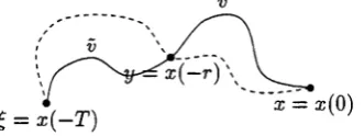
Figure 1.2: W( x ) A pproxim ation for a L im it Cycle System Worst C a se Trajectory

C ontours of W(x)

F igure 1.3: A W orst Case T rajecto ry and th e C ontours of a W( x ) A pproxim ation F u rth erm o re, W{ x ) also decreases along reverse tim e w orst case tra jec to rie s cor responding to th e an tistabilizing PD E solution E ^ ( £ ,x ) . Hence, th e argm in of W( x )

forms an invariant set to which b o th forw ard and reverse tim e worst case tra jec to rie s

are a ttra c te d . Consequently, worst case tra jec to rie s te n d to s ta te s for which Vf>(x) a n d

V ^ (£ ,x ) have equal gradients (w ith respect to x, if th ey ex ist), ra th e r th a n to any

m in im a of either function. Note th a t in th e ^2-gain analysis case it is th e zero avail

able power th a t guarantees th a t the sta te s of com m on gradient and com m on m in im a

(26)

1.5 O p tim a l S ta t e F ee d b a ck P o w er G ain C o n tr o l

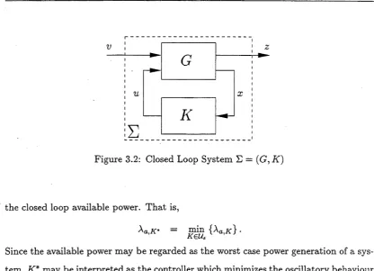
A closed loop system consisting of a plant G and a controller K is an example of a system with an input and output. Consequently, the input / output system (G :K) may be analysed using the power gain analysis techniques outlined thus far.

Figure 1.4: Closed Loop System E = (G , K)

Since the controller K modifies the behaviour of system (G , K), it is reasonable to expect th at different choices of controller K may yield different levels of internal power generation, and hence different values of available power. Thus, we may associate with system (G , K) the available power Aa, K , which is dependent on the choice of controller

K. Furthermore, since the available power is always bounded below by zero, 0 < min{Aa.^} < \ a. K,

K

for any controller K. Hence, it is feasible to define an optimal state feedback power gain control problem which involves finding an optimal controller K* such th at

Aa.K* = min {Au.k} ■

As the available power Aa, K may be interpreted as a measure of the worst case nonzero steady state behaviour of system ( G, K) , it is clear th at the optimal state feedback controller is desirable in that it seeks to minimize the closed loop “oscillatory” behaviour of the system. Indeed, if the nonlinear state feedback "H^-control problem is solvable, then the optimal state feedback power gain control problem will yield the optimal state feedback /H(X) controller K* with Xa,K* = 0 and the closed loop (G ,K*) asymptotically stable.

[image:26.534.168.354.229.350.2]

(27)

1.6 T h e s is O u tlin e 11

can be found by computing the solution of a corresponding Hamilton-Jacobi-Isaacs equation [16].

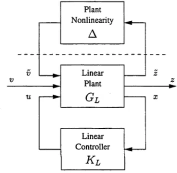
Using this method of solution, the synthesis of optimal state feedback power gain controllers for a class of linear plants with actuator nonlinearities is considered. Typ ically, we find that the optimal controller attem pts to invert the actuator nonlinearity in the spirit of Inverse Control [40].

1.6 T h e s is O u tlin e

The following list summarizes the chapter by chapter content of this thesis:

C hapter 2 The theory of power gain analysis is developed for a large class of nonlinear

dynamical systems.

C hapter 3 The analysis ideas of Chapter 2 are broadened further to investigate the

applicability of power gain analysis to the problem of state feedback controller synthesis.

C hapter 4 The issue of computing appoximations for the candidate power bias /

storage function pairs proposed in Chapter 2 is addressed.

C hapter 5 The richness of behaviour of explicit nonlinear systems with power gain is

investigated, revealing a real departure from the known behaviour of nonlinear systems with finite ZVgain.

C hapter 6 The contributions of this thesis are summarized. Further work in this new

research area is detailed.

1 .7

S u m m a r y o f C o n tr ib u tio n s

The principal contributions of this thesis are listed below.

• Generalization of the C2-gain inequality to the power gain inequality.

• Analysis of the stability of nonlinear systems with power gain, in the absence of disturbances.

(28)

• In te rp re ta tio n of th e power gain inequality using a finite horizon calculus of vari

atio n s problem .

• T h e concept of available power for nonlinear system s w ith power gain.

• G eneralization of energy dissip ativ ity to power dissipativity, th ereb y including

nonlinear system s w ith power gain.

• C oncepts of available storage a n d required supply for nonlin ear system s w ith

power gain.

• A nalysis of th e sta b ility of nonlinear system s w ith power gain, in th e presence of

th e w orst case d istu rb an ce.

• F o rm ulation of th e op tim al s ta te feedback power gain control problem , w ith a p

plicatio n to linear system s w ith a c tu a to r nonlinearities.

(29)

C h a p te r 2

C o n tin u o u s T im e P o w e r G a in

A n a ly s is

2.1 I n tr o d u c tio n

M any nonlinear system s, such as lim it cycles system s, exh ibit internal power generation

which is m anifested in th e persistence of o u tp u ts in the absence of distu rb ances. Since

such system s produce an infinite am ount of energy, tre a tm e n t using s ta n d a rd energy

gain analysis techniques is not possible.

In ord er to overcome th is lim itation in th e theory, we propose a generalization of

energy gain to include system s w ith power gain. B y developing concepts such as power

dissipativity, a theo ry of power gain analysis is established.

2 .2

C la ss o f S y s te m s

T h ro u g h o u t this ch ap ter, we are concerned w ith th e analysis of nonlinear of th e form

w here rr(0) = x E R n is th e initial sta te , x(t) E R n is th e sta te a t tim e t, v(t) E R p is th e d istu rb an c e , and z(t) E R 9 is th e o u tp u t. To sim plify n o tatio n , th e unpenalized will be w ritte n as <p(t, to, xq', v), where xo is th e initial s ta te corresponding to th e initial tim e to, t is th e cu rren t tim e, and v is the d istu rb an ce. W here the initial sta te , initial

x(t) = a(x(t)) + b(x(t))v(t), z ( t) = h ( x ( t))

(2.1)

ru n n in g cost will be d enoted by c(x) = \h(x)\2. T he flow or tra je c to ry of system E

(30)

14 C h a p te r 2. C o n tin u o u s T im e P o w e r G a in A n a ly s is

tim e, and d istu rb an ce are clear from th e context, this will be a b b re v iate d to x(t).

A nu m ber of definitions of reach ab ility of th e s ta te space of system s are required.

D e f in it io n 2 .2 .1 (C o m p le t e R e a c h a b ility ) A subset X of the state space of system

E is completely reachable if for any x' ,x" E X , there exists a time horizon 0 < T < oo

and a disturbance v E £2(0, T\ such that <p(T, 0, x'\ v) = x" with cp(t, 0, x'\ v) E X for allf E [0, T~\.

D e f in it io n 2 .2 .2 (U n ifo r m C o m p le te R e a c h a b ility ) A subset X of the state space of system E is uniformly completely reachable if there exists a finite nonnegative map ping Txy : I xI - 4 R and a mapping ux<y(s) : I x I x R - } R p such that for any x,

y £ X , E T2[0, 5 0, x, vX y) y, and Tx,y , 11222[0.^7V, bounded

on compact subsets of X x X .

T he following definition of local uniform reachability is a generalization of t h a t found

in [2].

D e f in it io n 2 .2 .3 (L o c a l U n ifo r m R e a c h a b ility ) The state space of system E is defined to be locally uniformly reachable if for each x' E R n , there exists a 5 > 0, and continuous functions a \ : [0,5) —> R ~ and a2 : [0,5) —» R ~ where aq(0) = 0 = <*2(0),

such that for any x" E R n with \\x" — x'\\ < 5, there exists finite time T > 0 and a disturbance v E £2[0,T ] such that ip(T,0,x']v) = x" and

IMl£2[0,T] < <*i(|x" - s ' l ) , (29)

T < Cl2(\x" - x'\).

W here necessary, th e class of system s E is fu rth e r restricted by th e following as

sum ptions.

( A l ) a, 5, a n d c are continous functions.

(A 2 ) T he s ta te space is C om pletely Reachable (D efinition 2.2.1).

(A 3 ) T he s ta te space is U niform ly C om pletely Reachable (D efinition 2.2.2).

(A 4 ) T he s ta te space is Locally U niform ly Reachable (D efinition 2.2.3).

(A 5 ) |a (x ) — a (p )| < L \\x — y\ for all xgy E R ” .

(31)

2.2 C la s s o f S y s t e m s 15

(A7) a{x) • x < — C \ \ x\2 + C2, for all x E R n, where C\ > 0, C2 > 0. (A8) a(x) ■ x > —C3|x|2 — C4, for all x E R n, where C3 > 0, C4 > 0.

(A9) Ib(x) — b(y)| < L2\x — y\ for all x,y G R 7'.

(A10) |fr(x)| < L3 for all x G R n.

( A l l ) |c(x) - c(y)\ < L4\x - y\ for all x,y G R n .

(A12) 0 < c(x) < L5(l + |^ |2) for all x G R n.

(A13) c(x) > L6(|x|2 - y) for all x G R n, where Lq > 0, y > 0.

(A14) c(x) —> 00as |x| —> 00.

(A15) The level sets of c(-) are compact.

When required for the proof of particular results, these assumptions will be cited indi vidually. Note th at some of the above assumptions follow from others, but are listed individually for clarity.

The continuity and Lipschitz assumptions (Al) and (A5) are required for existence of solutions to the differential equation (2.1).

Proposition 2.2.4

(i) A ssum ptions (A l) and (A5) im ply assumption (A6). (ii) A ssum ptions (A l) and ( A l l ) im ply assumption (A12). (Hi) A ssum ption (A6) implies assumption (A8).

Proof: Applying assumption (A5),

|a(x)| = \a(x) - a(y) + a(y)\ < |a(x) — a(y)| + |a(y)| < Li\x - y\ + \a(y)\

< m ax (L i,|a(y )|) (1 + \x — y|).

Continuity assumption (Al) implies that for any y G R n , |a(y)| < 00. Choosing y — 0

(32)

Also,

a(x) ■ x > —|a(ar)||x| > —L i ( l + |x |)|x

using assu m p tio n (A6) and th e fact th a t \x\2 — 2\x\ + 1 > 0. B u t, this is ju s t assu m p tio n

(A8). Hence, assu m p tio n (A6) implies (A8), which proves (Hi). ■

A ssu m p tio n (A7) is a stab ility assu m p tio n th a t ensures the existence of an a ttra c tin g

set for th e u n p e rtu rb e d dynam ics of system (2.1).

A ssum ptions (A9) an d (A10) are Lipschitz a n d boundedness assum ptions resp ec

tively, an d consequently independent.

A ssum p tio n (A13) provides a lower b ound for th e growth of th e unpenalized ru n n in g

cost for th e system . A ssu m p tion (A14) ensures th a t th e sta te of th e system cannot te n d

to oo while incurring only a finite unpenalized running cost, w hilst assu m p tio n (A15)

ensures t h a t sequences of sta te s w ith uniform ly bounded unpenalized ru n n in g cost are

confined to a closed a n d b o u n d ed set. A ssum ptions (A14) and (A15) m ay b e regarded

as effectively d e te c ta b ility assum ptions.

P r o p o s it io n 2 .2 .5

(i) Assumption (A13) implies assumption (A14). (ii) Assumption (A13) implies assumption (A15).

(Hi) Assumptions ( A l) and (A14) imply assumption (A15).

P r o o f: T h e proof of (i) is im m ediate. To prove (ii), define th e level sets

Kl = {x e R n : c(x) < L} , (2.3)

Ml = {x € R" : U ( \ x \ 2

(33)

2.2 C lass o f S y ste m s 17

Finally, suppose that assumption (A14) holds. That is, c(x) —> oo as jm| —> oo. So, given M > 0, there exists X > 0 such that

Hence, applying the definition of Km (2.3), x G Km implies th at |x| < X . That is, Km Q B[0; X]. Now, choose any L such that infx€Rn {c(x)} < L < M. x G Kl implies

that c(x) < L < M . Hence, Kl Q Km Q ß[0;X ]. T hat is, Kl is a bounded set. Suppose th at assumption (Al) holds, so that c(-) is continuous. Then, Kl is closed by definition. Hence, Kl is compact. So, this demonstrates th at Kl is compact for any

L < M , where M is fixed arbitrarily large. That is, assumption (A15) holds.

So, assumptions (Al) and (A14) imply (A15), proving (iii). ■

If the disturbance appears explicitly in each component of the state equation of system (2.1), intuitive it is expected that the state space of the system will be reachable. The following simple result states that indeed the three defined forms of reachability hold (Definitions 2.2.1, 2.2.2, and 2.2.3).

T heorem 2.2.6 Suppose that system S satisfies assumption (A6) with state equation

of the form

where b G R is a nonzero constant. Then, reachability assumptions (A2), (A3), and

(A4) hold.

Proof: Let M be any compact subset of the state space of system S, Rn. Let x,

y G M, and define the trajactory

|arI > X =$■ c{x) > M.

Contrapositively,

c{x) < M =$■ \x\ < X.

x = a(x) + bv

(2.4) Clearly x(0) = x and x(y/\y — x\) = y. So, define

T (x,y ) = V|j/ - x|. (2.5)

(34)

so th a t

v { x , y , s ) y - x — a \ x + y - x

V \ y ~ c

(2.6)

V \ y ~ x\

T h a t is, v { x , y , s ) drives th e system from s ta te x to y in tim e T { x , y ) . Now, applying th e trian gle ineq u ality and assu m p tio n (A6),

\ v ( x , y , s ) I < — y - x

s iii

*

h

V\y

-V\y ~ x

+ a \ x + y - x

V\y - :

1 + \x\2 + y/ \ y — x\ s

V\y

- x \ + L i ( l + \ x\2 + \ x - yI) : L { x , y ) ,

for all s G [0 ,T (x ,y )]. Clearly L ( x , y) is uniform ly b o un ded on com pact sets. Hence,

\\v(x>y,-)\\2

c2

^

L(x,y)2V\y - x\ <

° ° ? (2-7)

T { x , y ) = y/ \ y - x\ < oo, (2.8) for all z , y G M . Inequalities (2.7) and (2.8) im m ediately im ply assu m p tio n (A2). Since these inequalities hold for any x, y in any com pact set M C R n , th e s ta te space of E m ust also be uniform ly com pletely reachable, (A3). F u rtherm o re, (2.7) an d (2.8)

define th e continuous functions a?i and c*2 in th e inequality (2.2) of D efinition 2.2.3.

Hence, th e s ta te space of E is also locally uniform ly reachable, (A4). ■

2 .3

T h e

C

2

an d

T V

sp a c e s

Conventional 'Hoc th eo ry is concerned w ith th e analysis of system s w ith resp ect to an

in p u t / o u tp u t energy ( £2-) gain property. C onsequently, th e fu n d am en tal n orm ed

linear space is th e £ 2 function space.

D efinition 2.3.1 The norm || • \\c2 is defined to be the energy of a signal. That is,

v(s)|2 dsj>. (2-9)

The space £ 2 is defined to be the space of all signals with finite £ 2 norm. That is,

£ 2 = {u : R K p I |M|£2 < 00} . (2.10)

As power gain analysis of system s will be concerned w ith the analysis of system s w ith

(35)

2.3 The £2 and T V spaces 19

sem i-norm ed linear T V (finite power) function space (see P ro po sition 2.3.5 for a proof of the sem inorm p ro p erty ).

D e fin itio n 2 .3 .2 The sem inorm || • \\jrj) is defined to be the average power o f a signal. That is,

\ Mt v = y ^ i m s u p j i ^ |u(s)|2 d s j . (2.11)

The space T V is defined to be the space o f all signals with fin ite T V sem inorm . That is,

T V = {v :R —» R£ I IMIjf-p < 00} . (2.12) R e m a r k 2 .3 .3 W ith regard to th e definitions of th e £2 and T V spaces, it is im p o rta n t to note th e use of a lim it in (2.9) and a lim it superior in (2.11). Since the integral

f Q |i;(s) |2 ds in (2.9) is a nondecreasing function of th e horizon T , clearly th e use of a lim it in (2.9) is sufficient to ensure th a t th e £2 norm is well defined. However,

th e fraction ^ |u (s) |2 ds in (2.11) does n o t enjoy th e same m onotonicity property. Hence, a sequence {Tk} which ten d s to infinity m ay resu lt in m ultiple clu ster points of th is fraction, resu ltin g in an undefined lim it (see E xam ple 2.3.4). To avoid this, a

lim sup is used in th e definition of th e sem inorm (2.11), thereby cap tu rin g a tight u p per

b o und for th e power of th e signal. ◄

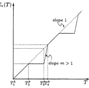
E x a m p le 2 .3 .4 In th is exam ple, a signal v G T V is c o n stru c te d such th a t PV(T ) := f 0T lv (s )l2ds evaluated along th e u nb ounded increasing sequence {Tk} has two cluster points.

Define E V( T) := f 0 ||u (s )||“ ds. Suppose th a t initially PV( T) is increasing tow ards an u p p er cluster point. For PV(T ) to have a second cluster p o in t, clearly PV( T) m ust decrease. Since PV{ T) = E-pr~ an d E V( T) is nondecreasing for all T , th is requires th a t

E V( T) increase a t a ra te slower th a n T . So, for th e purpo se of th is exam ple, choose v

co n stan t in some interval, as illu strate d in Figure 2.1.

In order to have two cluster points of th e sequence Pv (Tk), th e d u ratio n T3 — m ust be sufficiently large such th a t PV( T) a tta in s a c o n sta n t lower b o u n d , for exam ple