Octupolar invariants for compact binaries on quasicircular orbits

This is a repository copy of

Octupolar invariants for compact binaries on quasicircular

orbits

.

White Rose Research Online URL for this paper:

http://eprints.whiterose.ac.uk/98000/

Version: Published Version

Article:

Nolan, P., Kavanagh, C., Dolan, S.R. orcid.org/0000-0002-4672-6523 et al. (3 more

authors) (2015) Octupolar invariants for compact binaries on quasicircular orbits. Physical

Review D (PRD), 92 (12). 123008. ISSN 1550-7998

https://doi.org/10.1103/PhysRevD.92.123008

eprints@whiterose.ac.uk https://eprints.whiterose.ac.uk/

Reuse

Unless indicated otherwise, fulltext items are protected by copyright with all rights reserved. The copyright exception in section 29 of the Copyright, Designs and Patents Act 1988 allows the making of a single copy solely for the purpose of non-commercial research or private study within the limits of fair dealing. The publisher or other rights-holder may allow further reproduction and re-use of this version - refer to the White Rose Research Online record for this item. Where records identify the publisher as the copyright holder, users can verify any specific terms of use on the publisher’s website.

Takedown

If you consider content in White Rose Research Online to be in breach of UK law, please notify us by

Octupolar invariants for compact binaries on quasicircular orbits

Patrick Nolan,1 Chris Kavanagh,1Sam R. Dolan,2 Adrian C. Ottewill,1Niels Warburton,3,1 and Barry Wardell1,4 1_{School of Mathematical Sciences and Complex & Adaptive Systems Laboratory,}

University College Dublin, Belfield, Dublin 4, Ireland

2_{Consortium for Fundamental Physics, School of Mathematics and Statistics, University of Sheffield,}

Hicks Building, Hounsfield Road, Sheffield S3 7RH, United Kingdom

3_{MIT Kavli Institute for Astrophysics and Space Research, Massachusetts Institute of Technology,}

Cambridge, Massachusetts 02139, USA

4_{Department of Astronomy, Cornell University, Ithaca, New York 14853, USA} (Received 13 August 2015; published 23 December 2015)

We extend the gravitational self-force methodology to identify and compute newO_{ðμÞtidal invariants} for a compact body of massμon a quasicircular orbit about a black hole of massM≫μ. In the octupolar sector we find seven new degrees of freedom, made up of 3_þ3 conservative/dissipative ‘_electric’ invariants and3_þ1‘_magnetic’_{invariants, satisfying}1_þ1and1_þ0trace conditions. We express the new invariants for equatorial circular orbits on Kerr spacetime in terms of the regularized metric perturbation and its derivatives; and we evaluate the expressions in the Schwarzschild case. We employ both Lorenz gauge and Regge-Wheeler gauge numerical codes, and the functional series method of Mano, Suzuki and Takasugi. We present (i) highly-accurate numerical data and (ii) high-order analytical post-Newtonian expansions. We demonstrate consistency between numerical and analytical results, and prior work. We explore the application of these invariants in effective one-body models and binary black hole initial-data formulations.

DOI:10.1103/PhysRevD.92.123008 PACS numbers: 95.30.Sf, 04.20.-q, 04.25.dg

I. INTRODUCTION

The prospect of ‘_{first light}’ _{at gravitational wave}

detectors has spurred much work on the gravitational two-body problem in relativity. It is now a decade since the first (complete) simulations of binary black hole (BH) inspirals and mergers in numerical relativity (NR)[1]. Such simulations have revealed strong-field phenomenology, such as ‘_superkicks’ _{[2], and have provided template}

gravitational waveforms. Yet, it may be argued, numerical relativity has also highlighted the‘_unreasonable

effective-ness’ _{of both post-Newtonian (PN) theory [3], and the}

effective one-body (EOB) model [4].

BH-BH binaries, and their waveforms, are described by parameters including the masses M, μ, spins, orbital parameters, etc. The parameter space expands for BH-neutron star (NS) binaries—a key target for detection in 2016[5]—_{as tidal interactions also play an important role}

[6,7]. Semianalytic models, such as the EOB model, allow for much finer-grained coverage of parameter space than would be possible with (computationally expensive) NR simulations alone. In addition, effective models can bring physical insight[8–10]. Forreal-timedata analysis it may be necessary to blend effective models with surrogate/ emulator models[11–13]and careful analysis of modeling uncertainties [14].

By design, the EOB model[15–19]incorporates under-determined functional relationships, which are‘_calibrated’

with PN expansions and numerical data. Recently, it was shown that invariant quantities computed via the

gravitational self-force (GSF) methodology [20–22] can be used for exactly this purpose[16,23–27]. In fact, as the GSF methodology is designed to provide highly-accurate strong-field data in the extreme mass-ratio regime[28,29], it provides complementary constraints to PN and NR approaches, which excel in the weak-field and comparable mass-ratio regimes, respectively[30]. Thus, new GSF data, nominally limited in scope to the extreme-mass ratio regime,μ=M≪1, may immediately be applied to enhance models of comparable-mass inspirals, required for data analysis at, e.g., Advanced LIGO[5].

In recent years, a growing number of invariant quantities, associated with geodesic orbits in black hole spacetimes perturbed through linear order O_{ðμ=MÞ, have been} extracted from GSF theory. For quasicircular orbits on Schwarzschild, these include (i) the redshift invariant [31,32], (ii) the shift in the innermost stable circular orbit [33], (iii) the periastron advance (of a mildly eccentric orbit) [33,34], (iv) the geodetic spin-precession invariant [26,35,36], (v) tidal eigenvalues [27,37,38], (vi) certain octupolar invariants [27,38]. Recently, (i) has been com-puted for eccentric orbits [34,39], and (i)–(ii) have been

computed for equatorial quasi-circular orbits on Kerr spacetime[40].

In 2008, the GSF redshift invariant at O_{ðμ=MÞ was} compared against a post-Newtonian series at 3PN order (i.e., O_ðv6_=c6

Þ) [31]. Many further PN expansions have followed for invariants (i)–(vi) at very high PN orders

(GSF) and analytical (PN) approaches has developed, enabling precise comparisons of high-order coefficients [36,37,41–43]. Such comparisons are invaluable in quality assurance, as they have been used to correct small errors in both GSF calculations [37] and PN expansions [36]. Furthermore, in the“_{experimental mathematics}”_approach

[41,44], high-order PN coefficients may be extracted in closed (transcendental) form from exquisitely-precise numerical GSF calculations.

The purpose of this paper is to classify and compute GSF invariants at “_octupolar” _{order, i.e., featuring three}

deriv-atives of the metric, or equivalently, first derivderiv-atives of the Riemann tensor. This sector has been previously considered by Johnson-McDanielet al.[45]and Bini & Damour[27], among others [46–49]. Our intention is to provide a complementary analysis which extends recent GSF work on the dipolar (spin precession) and quadrupolar (tidal) sectors. We aim for completeness, by (i) seeking a complete basis of octupolar invariants, (ii) providing both numerical GSF data and high-order PN expansions at O_ðμ=MÞ.

In outline, the route to obtaining invariants is straightfor-ward: (1) in the GSF formulation, the motion of a small compact body is associated with a geodesic in a regularly-perturbed vacuumspacetime [50,51]; (2) the electric tidal tensorE_{abof the regularly-perturbed spacetime defines an} orthonormal triad at each point on the geodesic; (3) the covariant derivative of the Riemann tensorRabcd;eresolved in this triad gives a set of well-defined scalar quantities

fχig; (4) the functional relationshipsχiðΩÞ, whereΩis the circular-orbit frequency, are free of gauge ambiguities; (5) we define the“_invariants”Δ_χiðΩ_{Þto be the}O_ðμÞparts of the differences χiðΩ;μÞ−χiðΩ;μ¼0Þ.

The article is organized as follows. In Sec. II, we introduce electric and magnetic tidal tensors of octupolar order; decompose in the“electric quadrupole”triad; exam-ine the “_background” _(μ¼0) quantities; and apply per-turbation theory to derive invariant quantities through O_ðμ_Þ. In Sec. III we describe various computational approaches for obtaining the regular metric perturbation hR

aband its associated invariants. In Sec.IVwe present our results, primarily in the form of tables of data and PN series. In Sec.Vwe outline two wider applications of our work. We conclude with a discussion of progress and future work in Sec. VI.

Conventions: We set G_¼c_¼1 and use the metric signature_þ2. In certain contexts where the meaning is clear we also adopt the convention that M¼1. General coor-dinate indices are denoted with Roman letters a; b; c;…, indices with respect to a triad are denoted with letters i; j; k;…_{, and the index 0 denotes projection onto the}

tangent vector. The coordinates _ðt; r;θ;ϕ_Þ denote general polar coordinates which, on the background Kerr space-time, correspond to Boyer-Lindquist coordinates. Covariant derivatives are denoted using the semi-colon notation, e.g., ka;b, with partial derivatives denoted with

commas. Symmetrization and antisymmetrization of indi-ces is denoted with round and square brackets, () and [], respectively. Calligraphic tensors (e.g.E_ab,B_ab) are sym-metric in their indices and tracefree.

II. FORMULATION

A. Fundamentals

1. Tidal tensors

We begin by considering a circular-orbit geodesic in the equatorial plane of the regularly-perturbed vacuum Kerr spacetimegabwith a tangent vectorua. From the Riemann tensorRabcd(equal to the Weyl tensorCabcdin vacuum) we can construct electric-type and magnetic-type“

quadrupo-lar”_tensors,

E_ab¼Racbduc_ud_{; ð2:1Þ}

B_ab¼R

acbducud; ð2:2Þ

whereRabcd¼ 1 2εab

ef_R

efcd. We may also construct“ octu-polar” _tensors,

Eabc¼Radbe;cudue; ð2:3Þ

Babc¼Radbe;cudue: ð2:4Þ

The quadrupolar tensors are symmetric (E_ab¼E_ba, B_ab¼B_{ba), tracefree (}Ba

a¼0 in general, Eaa¼0 in vacuum) and transverse (E_abub

¼0_¼B_abub_{). The} octu-polar tensors are symmetric, and traceless in the first two indices (as Rabcd ¼Rcdab and Rab¼Rcacb¼0) in vac-uum. By contracting the Bianchi identity (or its dual) Rabcd;eþRabde;cþRabec;d¼0, we observe that the octu-polar tensors are also traceless on the latter pair of indices, Eabb¼0¼Babb, in vacuum. Note however that the octupolar tensors are not symmetric in the latter pair of indices, in general.

2. Tetrad components

Let us now introduce an orthonormal tetrad_fea

0¼ua; eαig on the worldline and define tetrad-resolved quantities in the natural way, so that

χi0j…¼χabc…eaiubecj…; ð2:5Þ

where χabc… is any tensor and i; j; k∈f1;2;3g. The

Eij0; Ei½jkŠ; and Eijk≡EðijkÞ; ð2:6Þ

and similarly in the magnetic sector.

Note that E_{ij is real and symmetric, and thus its} eigenvalues are real and its eigenvectors are orthogonal. Thus, we may select our triad ei

a to coincide with the electric-quadrupolar eigenbasis. In other words, we choose the triad in whichE_{ij is diagonal. We choosee}a

2 to be the vector orthogonal to the equatorial plane.

3. Equatorial symmetry

For circular equatorial orbits, the reflection-in-equatorial plane symmetry implies that many components are iden-tically zero. Namely,

E_12¼E_23¼B_11¼B_13¼B_22¼B_33¼0; ð2:7Þ

E112¼E222¼E233¼E123¼0; ð2:8Þ

B111¼B122¼B133¼B113¼B223¼B333¼0; ð2:9Þ

with all permutations of these indices also zero.

B. Classification of octupolar components

Now we consider the three types of terms (2.6) sepa-rately, and show that Eij0, Bij0 and Ei½jkŠ, Bi½jkŠ may be derived from dipolar and quadrupolar terms, whereas E_ijk≡E_ðijk_Þ, Bijk≡B_ðijk_Þ encode new information at

octupolar order.

1. Eij0and Bij0

For circular orbits, we have ub_ea

1;b¼ωea3, ubea2;b¼0 andubea_3;b¼−ωea1, where ωis the precession frequency with respect to proper time, defined by parallel transport observed from the electric eigenbasis (cf. Refs. [35,37]). As the quadrupolar eigenvalues are time-independent on circular orbits, the only nontrivial components are

E130¼ωðE11−E33Þ; B120¼−ωB23;

B230¼ωB12: ð2:10Þ

2. Ei_½jk_Š and Bi_½jk_Š

By virtue of the Bianchi identity,

Ea_½bc_Š¼− 1 2u

e

ðud_R

dabcÞ;e; Ba_½bc_Š¼− 1 2u

e

ðud_R dabcÞ;e:

ð2:11_Þ

We now (i) project onto the tetrad, (ii) use that B_ij¼ 1

2ϵjklR0ikl and Eij ¼−12ϵjklR0ikl, and (iii) recall that the tetrad components in the electric frame are constants for circular orbits. Thus all components are zero except

E2_½23_Š¼E1_½31_Š¼ 1

2ωB23; ð2:12Þ

E3_½31_Š¼E2_½12_Š¼− 1

2ωB12; ð2:13Þ

B1_½12_Š¼B3_½23_Š¼ 1

2ωðE11−E33Þ; ð2:14Þ

and permutations thereof.

3.E_{ijk and} B_ijk

In general, E_{ijk and} B_{ijk each have ten components} satisfying 3 trace conditions, i.e., seven independent components each. For circular orbits, 4 electric and 6 magnetic components are zero, respectively, leaving 6 and 4 nontrivial quantities satisfying 2 and 1 nontrivial trace conditions. In other words, there are 10 quantities we may calculate (given below), satisfying 3 nontrivial trace con-ditions; thus, 7 new independent degrees of freedom at octupolar order.

4. Additional invariants

Other octupolar quantities may be written in terms of the set identified above. For example, a relevant quantity in EOB theory [see Ref.[27], Eq. (D10)] isK3_þ≡EabcEabc, which may be expressed as

K3_þ¼E2111þE 2

333þ3ðE 2 122þE

2 133þE

2 311þE

2 322Þ

−6E2

130; ð2:15Þ

whereE_130¼1 3E130.

C. Circular orbits: Background quantities

Below we give the values of the tidal quantities for circular equatorial geodesics on the unperturbed Kerr spacetime, i.e., for test-masses (μ_¼0). Here, the orbital radius isr0and the orbital frequency isΩ¼

ffiffiffiffiffi M

p

=ðr3=20 þ a ffiffiffiffiffi

M

p

Þ where a is the Kerr spin parameter and a >0 (a <0) for prograde (retrograde) orbits.

The tangent vectorua _{and electric-eigenbasis triad have} the components[52]

ua _{¼ ½U;0;0;ΩUŠ; ð2:16aÞ}

ea 1¼ ½0;

ffiffiffiffiffiffi

Δ₀

p

=r0;0;0Š; ð2:16bÞ

ea

2¼ ½0;0;1=r0;0Š; ð2:16cÞ

ea

3 ¼−ϵabcdubec1ed2; ð2:16dÞ

whereU¼ ffiffiffiffiffi M

p

=ðΩ_r3=2

υ2_≡1−3M=r 0þ2a

ffiffiffiffiffi M

p

=r3=20 : ð2:17Þ

The spin precession rate is ω_¼ ffiffiffiffiffiffiffiffiffi Mr0

p

=r2 0.

1. Quadrupolar components

The (nontrivial) quadrupolar components are

E_11¼M r3 0

−3MΔ0 υ2r5

0

; ð2:18aÞ

E_22¼−2M

r3 0

þ3MΔ0

υ2_r5 0

; _ð2:18b_Þ

E_33¼M r3 0

; ð2:18cÞ

B_12¼−3M

3=2 ffiffiffiffiffiffi_Δ 0

p

ð1−a= ffiffiffiffiffiffiffiffiffi Mr0

p Þ

r9=20 υ

2 ; ð2:18dÞ

We note thatB_23¼0 on the background.

2. Octupolar components

In the electric sector,

E_{111¼ þ}A_ð6r2

0−9Mr0−12a ffiffiffiffiffiffiffiffiffi Mr0 p

þ15a2

Þ ð2:19Þ

E_122¼−A_ð3r2

0−2Mr0−16a ffiffiffiffiffiffiffiffiffi Mr0 p

þ15a2

Þ ð2:20Þ

E_133¼−A_ð3r2

0−7Mr0þ4a ffiffiffiffiffiffiffiffiffi Mr0 p

Þ; ð2:21Þ

where A_¼ ffiffiffiffiffiffi_Δ 0

p

M=_ðr7 0υ

2

Þ. We note that E_311¼E_322¼ E_333¼0 on the Kerr background.

In the magnetic sector,

B_{211¼ þ}C_ð4r2

0−8Mr0þ7a2Þ

−D_ð4r2

0−7Mr0þ5a2Þ; ð2:22Þ

B_222¼−C_ð3r2

0−6Mr0þ9a2Þ

þD_ð3r2

0−4Mr0þ5a2Þ; ð2:23Þ

B_233¼−C_ðr2

0−2Mr0−2a2Þ

þD_ðr2

0−3Mr0Þ; ð2:24Þ

where C_¼2M3=2_=ðr13=2 0 υ

2

Þ and D_¼3aM=ðr7 0υ

2

Þ. Note that B_123¼0 on the Kerr background.

The“_derived”_{quantitiesEij0,Ei½jkŠ, etc., may be easily}

calculated using Eq. (2.10), Eq. (2.12)–(2.14) and

Eq. (2.19)–(2.24). For example, in the Schwarzschild

(a¼0) case, using Eq. (2.15)yields

K3_þ¼ 6M2

ð1−2M=r0Þð15r02−46Mr0þ42M2Þ r10

0 ð1−3M=r0Þ2

:

ð2:25Þ

D. Circular orbits: Perturbation theory

Here we seek expressions for the octupolar quantities in the regular perturbed spacetimeg¯abþhRab, whereg¯abis the Kerr metric in Boyer-Lindquist coordinates, and hR

ab¼ O_{ðμÞ is the} “_regular” _{metric perturbation defined by}

Detweiler and Whiting [50]. We work to first order in the small massμ, neglecting all terms atO_ðμ2

Þ, and noting that the regular perturbed spacetime is Ricci-flat.

We take the standard two-step approach[31,32,37]. For a given geodesic quantityχ(e.g.E₁₁₁), we first compareχon a circular geodesic in the perturbed spacetime withχ on a circular geodesic of the background spacetime at the same coordinate radiusr_¼r0. Then, noting thatr0itself varies under a gauge transformation atO_ðμ_Þ, we apply a correc-tion to compareχ on two geodesics which share the same orbital frequencyΩ.

Following the convention of Ref. [37], we use an

“_overbar”_{to denote}“_background”_{quantities, so that barred}

quantities such as u¯a _{are assigned the same coordinate} values as in Sec.II C. We useδto denote the difference at O_ðμ_Þ, i.e.,δeai ≡eai −e¯ai. AtOðμÞ,δmay be applied as an operator with a Leibniz rule δ_ðAB_{Þ ¼ ð}δA_ÞB_þAδB. In general, such differences are gauge-dependent. To obtain an invariant difference, we introduce the “

frequency-radius” _{rΩ via}

Ω_¼pffiffiffiffiffi_M=ðr3=2_{Ω þa}pffiffiffiffiffi_{MÞ: ð2:26Þ}

Then, we write

χ_ðrΩÞ−χ¯ðrΩÞ ¼Δχðr0Þ þOðμ2Þ: ð2:27Þ

Here χ¯_ðrΩÞ has the same functional form as χ on the

background spacetime, withr0replaced byrΩ. AsΔχis at

O_{ðμÞ, we may parametrize}Δ_{χusing the}O_ðμ0

Þbackground radiusr0, rather thanrΩ, asr0−rΩ¼OðμÞ. Such

relation-ships,Δ_{χðr0Þ, are invariant within the class of gauges in} which the metric perturbation is helically symmetric (implying thatu¯c_hR

ab;c ¼0 at the relevant order).

1. Perturbation of the tetrad

We may write the variation of the tetrad legs in the following way,

δua

¼β00u¯aþβ03e¯a3; ð2:28aÞ

δea

i ¼βi0u¯aþ X

3

j_¼1

with the coefficientsβab¼OðμÞto be determined below. First, we note thatβ00 andβ03 may be found by recalling key relations previously established in GSF theory for equatorial circular orbits on Kerr spacetime [31,53], namely,

δut ¯ ut ¼

1

2h00− ¯

Ω

2 ffiffiffiffiffi r0 M r

ðr2

0þa2−2a ffiffiffiffiffiffiffiffiffi Mr0 p

ÞF~r; ð2:29Þ

δuϕ ¯ uϕ ¼

1 2h00−

1 2Mðr

2

0−2Mr0þa ffiffiffiffiffiffiffiffiffi Mr0 p

ÞF~r: ð2:30Þ

Hereh00≡hRabu¯au¯b, andF~r≡μ−1Fr¼OðμÞis the (spe-cific) radial self-force given by

~ Fr¼

1

2u¯ a_u¯b∂h

R ab ∂r

_r

¼r0

: ð2:31Þ

Hence we have β00¼12h00 and β03¼−12 ffiffiffiffiffiffiffi r0Δ₀

M q

~ Fr. The diagonal coefficients βii follow from the normalization condition,_ðg¯abþhRabÞðe¯ai þδeaiÞðe¯bjþδebjÞ ¼δij. That is,

βii¼−12hii, where hii¼h R

abe¯aie¯bi (no summation over i

implied). From orthogonality of legs 0 and 3, we have

β30¼β03þh03 whereh03¼hRabu¯ae¯b3. By similar reason-ing,β10¼h01 andβ31þβ13þh13¼0. To eliminate the residual rotational freedom in the triad atO_{ðμÞ, we now} impose the condition that the triad is aligned with the electric eigenbasis, i.e., thatE_{ijis diagonal in the perturbed} spacetime (so that, e.g., E_13¼0). From this condition it follows that

β13¼ð

δR_Þ1030−E¯11h13 ¯

E₁₁−E¯₃₃ ; ð2:32Þ

β31¼

−_ðδRÞ1030þE¯33h13 ¯

E₁₁−E¯₃₃ ; ð2:33Þ

where

ðδR_Þ1030¼δRabcde¯a1u¯be¯c3u¯d: ð2:34Þ

2. Perturbation of octupolar components

Here we present results for the perturbation of the (symmetric tracefree) octupolar components E_ijk and B_ijk. The electric components are

δE_{111¼ ð}δ∇RÞ_ð10101_Þþ

h00− 3

2h11

¯

E_111þ2β03R¯10131; ð2:35aÞ

δE_{122¼ ðδ∇RÞ}

ð10202_Þþ

h00− 1

2h11−h22

¯

E_122þ2β03R¯10232; ð2:35bÞ

δE_{133¼ ð}δ∇RÞ_ð10303_Þþ

h00− 1

2h11−h33

¯

E_133þ2β03R¯10333þ 2

3β30ω¯ð ¯

E₁₁−E¯_{33Þ; ð2:35cÞ}

δE_{113¼ ð}δ∇RÞ_ð10103_Þþ 2

3β10ω¯ð ¯

E₁₁−E¯_{33Þ þ}β31E¯111þ2β13E¯133; ð2:35dÞ

δE_{223¼ ðδ∇RÞ}

ð20203_Þþβ31E¯122; ð2:35eÞ

δE_{333¼ ðδ}∇RÞ_ð30303_Þþ3β31E¯133; ð2:35fÞ

where

ðδ∇R_Þði0j0k_Þ¼δRabcd;eu¯bu¯de¯ð a i e¯cje¯

e_Þ

k; ð2:36Þ

¯

R_i0j3k¼R¯_abcd;eu¯ðb_e¯dÞ 3e¯ð

a i e¯cje¯

e_Þ

k: ð2:37Þ

The magnetic components are

ðδB_{Þ211¼ ð}δ∇RÞ20101þ

h00−h11− 1

2h22

¯

ðδB_{Þ222¼ ð}δ∇RÞ20202þ

h00− 3 2h22

¯

B_222þ2β03R¯20232; ð2:38bÞ

ðδB_{Þ233¼ ðδ∇RÞ} 20303þ

h00−

1

2h22−h33

¯

B_233þ2β03R¯20333þ 2 3β30ω¯

¯

B_{12; ð2:38cÞ}

ðδB_{Þ123¼ ðδ∇RÞ}

10203þβ13B¯233þβ31B¯211þ 1

3β10ω¯ ¯

B_{12; ð2:38dÞ}

where

ðδ∇RÞ_ði0j0k_Þ ¼δRabcd;eu¯bu¯de¯ð a i e¯cje¯

eÞ

k; ð2:39Þ

¯

R_i0j3k¼R¯_abcd;eu¯ðb_e¯dÞ 3e¯ð

a i e¯cje¯

e_Þ

k: ð2:40Þ

3. Invariant relations

As noted above, the coordinate radius of the orbit, r¼r0, is not invariant under changes of gauge [i.e., coordinate changes atO_ðμ_Þ]. On the other hand, the orbital frequencyΩis invariant under helically symmetric gauge transformations. Following Eq. (2.27), we may therefore express the functional relationship betweenχ∈_fE_111;…_g

andΩ_{as follows,}

χ_ðrΩÞ ¼χ¯ðrΩÞ þΔχðr0Þ þOðμ2Þ; ð2:41Þ

whererΩis the frequency-radius defined in Eq.(2.26), and

Δ_{χ ¼}O_ðμ_Þ. Note that χ¯_ðrΩÞ denotes the “test-particle”

functions defined in Sec.II Cevaluated atrΩ. By definition,

we haveΔΩ_¼0. At O_ðμÞ,

Δ_χ¼δχ−δΩdr0 dΩ¯

dχ¯ dr0

; _ð2:42_Þ

or, making use of Eq. (2.29) and (2.30) and

δΩ₌Ω¯ _¼δuϕ_=u¯ϕ_−δut_=u¯t_,

Δ_{χ ¼δχ}− 1

3Mr 3 0υ

2_F~ r

dχ¯ dr0

: ð2:43Þ

In summary, Δ_{χ defined by Eq. (2.43), Eq. (2.35) and} Eq. (2.38) are the invariant quantities which we will compute in the next sections.

4. Further quantities

In Sec.II Bwe wroteEij0,Ei_½jk_Š,Bij0,Bi_½jk_Šin terms of quadrupolar tidal components, and the spin precession scalar ω. If required, one may deduce the variation of these components by applyingΔ_{as a Leibniz operator. For} example, starting with Eq. (2.10),

ΔE_130¼Δ_ωðE¯₁₁−E¯_{33Þ þ}ω¯_ðΔE₁₁−ΔE_{33Þ: ð2:44Þ}

Numerical data for the variation in the quadrupolar com-ponentsΔE_11;…_;ΔB_21;…_{is given in Table I of Ref.[37].}

We may computeΔωfrom the redshift and spin-precession invariants,Δ_UandΔ_ψ, using

Δ_ω¼ω¯

¯ UΔU−

¯

UΩ Δ¯ _{ψ; ð2:45Þ}

together with the data in Table III of Ref.[37].

Similarly, the variationΔ_K3þ, for example, can be found by applyingΔ_{in this manner to Eq.(2.15). This can then be} related to the quantityδˆK3_þ, whose post-Newtonian expan-sion was given to7.5PN in Ref.[27]. Noting that K3_þ≡

Γ4_K 3_þ and

Γ_¼ 1

ffiffiffiffiffiffiffiffiffiffiffiffiffiffiffiffiffiffiffiffiffi 1−3M=r0 p

1_þ1

2h00þOðμ 2

Þ

; _ð2:46_Þ

we then have a relation between the first-order perturbations,

Δ_K3þ

¯ K3_þ ¼

ˆ

δK3_þþ2h00: ð2:47Þ

III. COMPUTATIONAL APPROACHES

In this section we outline our methods for computing the octupolar invariants for a particle of massμon a circular orbit of radius r0 in Schwarzschild geometry. Our approaches break into two broad categories: (i) numerical integration of the linearized Einstein equation in either the Regge-Wheeler (RW) or Lorenz gauge and (ii) analytically solving the Regge-Wheeler field equations as a series of special functions via the Mano-Suzuki-Takasugi (MST) method. In both cases we decompose the linearized Einstein equation into tensor-harmonic and Fourier modes and solve for the resulting decoupled radial equation. In this section, and subsections that follow,landmare the tensor-harmonic multipole indices, ω is the mode frequency and we work with standard Schwarzschild coordinates

ðt; r;θ;φ_Þ. For this section let us also define f≡f_ðr_{Þ ¼} 1−2M=r. We shall also use a subscript “₀” _{to denote a}

quantity evaluated at the particle. Finally, note that for a circular orbit about a Schwarzschild black hole the par-ticle’_{s (specific) orbital energy and angular-momentum are}

E0¼

r0−2M ffiffiffiffiffiffiffiffiffiffiffiffiffiffiffiffiffiffiffiffiffiffiffiffi r0ðr0−3MÞ

p ; L0¼r0

ffiffiffiffiffiffiffiffiffiffiffiffiffiffiffiffiffi M r0−3M s

; _ð3:1_Þ

respectively.

For calculations in the RW gauge there is a single

“master” radial function, _Ψlmω, to be solved for each tensor-harmonic and Fourier mode [54,55]. For circular orbits the Fourier spectrum is discrete and given by ω≡

ωm¼mΩ where Ω¼

ffiffiffiffiffiffiffiffiffiffiffi M=r3 0 q

is the azimuthal orbital

frequency. Consequently, we label the RW master function with only lm subscripts hereafter. The full metric pertur-bation can be rebuilt from the Ψlm’s and their derivatives [56]. Forl≥2the ordinary differential equation that Ψlm obeys takes the form

_d2

dr2 þ ½

ω2m−Ulðrފ

Ψlm¼S1δðr−r0Þ þS2δ0ðr−r0Þ;

ð3:2_Þ

where r is the radial “_tortoise” _{coordinate given by}

dr=dr¼f−1 _{and U}

ðrÞ is an effective potential. The effective potential used depends on whether the

perturbation is odd or even parity. For the odd/even parity modes, equivalently lþm¼odd=even, the potential is given by

Uo lðrÞ ¼

f r2

l_ðl_þ1_Þ−6M

r

; _ð3:3_Þ

Ue lðrÞ ¼

f r2

Λ2

2λ2

λ_þ1_þ3M r

þ18M

2

r2

λ_þM

r

;

ð3:4Þ

respectively, where λ_{¼ ð}lþ2_Þðl−1_Þ=2 and _Λ¼λ_þ

3M=r0. The form of the source terms, Si, also differs for the even and odd sectors. Explicitly, the odd sector sources take the form[57]

So

1¼−

2pf0L0

λlðlþ1_ÞXϕðθ;ϕÞ; ð3:5Þ

So

2¼

2pr0f20L0

λl_ðl_þ1_Þ Xϕðθ;ϕÞ: ð3:6Þ

For the even sector, we have

Se

1¼ pqE₀ r0f0Λ

_L2 0 E2 0

f2

0Λ−ðλðλþ1Þr 2

0þ6λMr0þ15M2Þ

Y

lmðθ;ϕÞ− 4pL2

0f 2 0 r0E0

ðl−2_Þ!

ðl_þ2_Þ!Yϕϕðθ;ϕÞ; ð3:7Þ

Se

2¼ ðr 2

0pqE0ÞYlmðθ;ϕÞ; ð3:8Þ

where we have defined the following expressions for convenience:

Xϕðθ;ϕÞ ¼sinθ∂θYlmðθ;ϕÞ; ð3:9Þ

Yϕϕðθ;ϕÞ ¼

∂_ϕϕþsinθcosθ∂_θþlðlþ1Þ 2 sin

2_θ

×Ylmðθ;ϕÞ ð3:10Þ

p_¼8πμ r2

0

; q_¼ f

2 0

ðλþ1_ÞΛ: ð3:11Þ

For the radiative modesl≥2,m≠0we will construct homogeneous solutions to Eq.(3.2)either numerically or as a series of special functions, as outlined in the subsections below. For the static (l≥2, m¼0) modes, closed-form analytic solutions to the homogeneous RW equation are known. In the odd sector these can be written in terms of standard hypergeometric functions:

~

Ψol0−¼x−l−12F1ð−l−2;−lþ2;−2l; xÞ ð3:12Þ

~

Ψol0þ ¼xl2F1ðl−1; lþ3;2þ2l; xÞ; ð3:13Þ

where hereafter an overtilde denotes a homogeneous solution, a “_þ” _{superscript denotes an outer solution}

(regular at spatial infinity, divergent at the horizon), a

“−” _{denotes an inner solution (regular at the horizon,}

divergent at spatial infinity) andx_¼2M=r. In practice, we need only solve the simpler odd sector field equations, and construct the even sector homogeneous solutions via the transformation[56]:

~ Ψelm ¼

1

λ_þλ2

3iωM

λ_þλ2

þ9M

2

ðr−2M_Þ r2

ðrλ_þ3MÞ

~ Ψolm

þ3Mfd ~ Ψolm

dr

: _ð3:14_Þ

Note this equation holds for both static and radia-tive modes.

a“_matching”_{procedure with the jump in the field and its}

derivative across the particle governed by coefficients S₁ andS_{2. Suppressing even/odd notation, we define} match-ing coefficients as follows:

D lm¼

1 Wlm

_S 1 f0þ

2MS₂

r2 0f20

Ψ∓lm−

S₂

f0 ∂_rΨ∓_lm

; _ð3:15_Þ

with the usual Wronskian defined as Wlm¼ f0ðΨ~

−

lm∂rΨ~þlm−Ψ~þlm∂rΨ~

−

lmÞ. Finally we construct the inho-mogeneous solutions via

Ψ

lmðrÞ ¼DlmΨ~lmðrÞ: ð3:16Þ

where the D_lm’s are constants for all values ofr.

To complete the metric perturbation in the RW gauge we use thel_¼0andl_¼1results of Zerilli[58]. Detweiler and Poisson expressed these contributions succinctly for circular orbits [59]. For the monopole and static dipole we have

hl¼0

tt ¼2μE0 ₁

rþ f r0−2M

Θ_{ðr−r0Þ; ð3:17Þ}

hl¼0 rr ¼

2μE0

rf2 Θðr−r0Þ; ð3:18Þ

hlt¼φ1;m¼0¼−2μL0sin2θ _r2_=r3

0 r < r0 1=r r > r0

; _ð3:19_Þ

where Θ is the Heaviside step function and all other components are zero. The l¼1, m¼1 mode does not contribute to our gauge invariant quantities so we will not give the explicit expression for the nonzerohtt,htr andhrr components of this mode (but as a check we use the expressions, given as Eqs. (5.1)–(5.3) in Ref.[59], to check

that the contribution from this mode to our invariants is identically zero).

As well as working in the RW gauge we also make a computation in the Lorenz gauge. Our code is a

Mathematica reimplentation of that presented by Akcay [60]and as such we refer the reader to that work for further details.

A. Numerical computation of the retarded metric perturbation

For our RW gauge calculation, as discussed above, analytic solutions are known for the monopole, dipole and static (m¼0) modes. This only leaves the radiative modes (l≥2, m≠0) to be solved for numerically. Our numerical routines are implemented inMathematicawhich allows us to go beyond machine precision in our calculation with ease. Given suitable boundary conditions near the black hole horizon and at a sufficiently large radius (we discuss below how we choose these radii in practice), we useMathematica’s NDSOLVEroutine to solve for the inner

and outer solutions to the homogeneous Regge-Wheeler equation (3.2). Inhomogenous solutions are then con-structed by imposing matching conditions of these func-tions at the location of the orbiting particle.

1. Numerical boundary conditions

In order to construct boundary conditions, we use an appropriate power law ansatz for _ΨRW in the asymptotic regions close to spatial infinity and the horizon, given by

~

Ψ∞RWðrÞ∼eiωr X

n_þ

n_¼0 an

ðωr_Þn; ð3:20Þ

~

ΨHRWðrÞ∼e−iωr X

n−

n_¼0

bnfðrÞn: ð3:21Þ

Recursion relations for the series coefficients can be found by inserting our ansatz into the homogeneous RW equa-tions, and choosing a maximum number of outer and inner terms nmax¼n gives us initial values for our fields at

these boundaries. Inserting(3.21)and(3.20)into(3.2)for the odd sector, we find the following recursion relations:

an¼ i

2n½ðlðlþ1Þ−nðn−1ÞÞan−1þ2Mωðn−3Þðn−1Þan−2Š; ð3:22Þ

bn ¼ 1

nðn−4iMω_Þ½ðlðlþ1Þ þ2nðn−1Þ−3Þan−1−ðnþ1Þðn−3Þan−2Š: ð3:23Þ

As discussed above we do not need to solve the even sector field equations as we can transform from the simpler odd sector solutions using Eq. (3.14).

For the inner homogeneous solutions, the convergence of the series (3.21) improves with increasing n−, and in

practice we choose n− ¼35. The outer solutions require

useful to add higher order terms. Note for a fixed max value n_þ the series will still converge with increasing r, as expected. After analysing this behavior, we taken_þ¼100 to get the best boundary conditions. Given the boundary expansions as a function ofr, for fixedn, we must then choose a location for our boundary sufficiently close to r_¼ ∞ to give the desired accuracy. Setting the final term in our ansatz to be of order 10−d_{, where d is our} desired number of significant figures, we choose as our boundaries:

r∞¼ ðan_þ10dÞ1=nþ; ð3:24Þ

rH ¼2Mþ ðbn−10

d_Þ−1=n−_: ð_3:25Þ

The expansions (3.21) and (3.20) give the boundary conditions in terms of an arbitary overall amplitude, specified bya0andb0. As we first construct homogeneous solutions we can set these amplitudes to any nonzero value, and in practice we choosea0¼b0¼1. The amplitudes are then fixed by the matching procedure described above.

2. Numerical algorithm

In this section we briefly outline the steps we take in our numerical calculation in the Regge-Wheeler gauge. The Lorenz-gauge calculation follows a very similar set of steps [60].

(i) For each lm-mode with l≥2 solve the odd sector RW equation, even if l_þm_¼even. For the radia-tive modes (l≥2,m≠0) calculate boundary con-ditions for the homogeneous fields at rH=∞ using

Eqs. (3.21) and (3.20). Using the boundary con-ditions, numerically integrate the homogeneous field equation(3.2)from the boundaries to the particle’_s

orbit at r¼r0. For the static modes (l≥2,m¼0) evaluate the static homogeneous solutions (3.12)–

(3.13) at the particle. Store the values of the inner and outer homogeneous fields and their radial derivatives atr0.

(ii) Forl≥2andlþm¼even transform from the odd sector homogeneous solutions to the even sector homogeneous solutions using Eq. (3.14).

(iii) For all modes with l≥2 construct the inhomo-geneous solutions via Eq. (3.16).

(iv) For the l≥2 modes reconstruct the metric pertur-bation using the formula in, e.g., Refs. [56]. (v) Complete the metric perturbation using the

monop-ole and dipmonop-ole solutions given in Eqs.(3.17)–(3.19).

(vi) Compute the retarded fieldl-mode (summed overm) contributions to the octupolar invariants using the formulas in Appendix A.

(vii) Construct the regularized l-modes using the tensor mode-sum approach described in Ref. [61]. The resulting contributions to the mode-sum accumulate rather slowly as l−2_.

(viii) Numerically fit for the unknown higher-order regu-larization parameters and use these to increase the rate of convergence of the mode-sum with l. This procedure is common in self-force calculations and is described in, e.g., Ref.[62].

(ix) To get the final result sum overland make the shift to the asymptotically flat gauge as discussed in AppendixB.

For r0≥4Mwe set the maximum computedl-mode to belmax¼80. This is sufficient to compute the octupolar

invariants to high accuracy—_{see Sec.IVfor details on the}

accuracy we obtain. For orbits with3M < r0<4Mwe find we need an increasing number ofl-modes to achieve good accuracy in the final results, and for orbits near the light-ring (located atr0¼3M) we setlmax¼130in our code—

see Sec.IV C.

B. Post-Newtonian expansion

The generation of analytic post-Newtonian expansions for the octupolar gauge invariants requires a calculation of the homogeneous solutions of the Regge-Wheeler equation for eachl_{mode. A general strategy for doing this was described}

in[63]. The calculation is broken into three sections: (i) the exact results of Zerilli give thel_¼0, 1 components of the metric—_{see Eqs.(3.17)–(3.19), (ii) certain} “_low-l”_values

calculated using the series solutions of Mano, Suzuki and Takasugi and (iii) “_high-l” _{contributions using a}

post-Newtonian ansatz. In a recent paper [43] this approach was optimized and improved allowing extremely high PN orders to be computed, which otherwise are only accessible by experimental mathematics techniques [41,42,64,65]. In the rest of this section we give a very brief overview of our technique and refer the reader to Ref.[43] for further details.

The analytic MST homogeneous solutions are expressed using an infinite series of hypergeometric functions denotedXin

lm, which satisfies the required boundary con-ditions at the horizon, and a series of irregular confluent hypergeometric functions, Xup_lm, satisfying the boundary conditions as r_→∞. Specifically we can write

Xin

lm∼Btranslm eþiωr; r→−∞

Xuplm∼Ctranslm e

−iωr_{; r} →∞

whereBtrans

lm andCtranslm are the complex constants known as transmission coefficients, so that, with a0¼b0¼1 in Eqs.(3.21) and(3.20), we have the identification

Xin

lm¼Btranslm Ψ~

H

RW ð3:26Þ

Xuplm ¼Ctranslm Ψ~

∞

RW: ð3:27Þ

natural and related small parameters, the frequency

ω_¼mΩ _{and the inverse of the radius, which is related} to the orbital frequencyΩ_byMΩ_¼pffiffiffiffiffiffiffiffiffiffiffiffiffiffiffiffiffi2GM=r3

. A natural way to deal with this double expansion is to instead expand in η_¼1=c, and introduce two auxiliary variables X1¼GM=r, X21=2¼ωr, so that each instance of X1 and X2 must each come with an η2 and are of the same order in the large-r limit. Expanding these solutions to a given PN order in this way amounts to truncating the Xin=up_{infinite series at a finite order. However an in depth}

analysis of the series coefficients and the sometimes subtle behavior of the hypergeometric functions reveals a struc-ture that can be exploited to optimize this truncation order and fine tune the length of the expansion of each term in the series.

A practical difficulty of this approach is that the MST series becomes increasingly large with higherη-order. For each PN ordery∼_r1

Ω∼η

2_{so that to get say 10 PN, we need}

20η powers. Significant further simplifications of these large series can be made rewriting the expansion as, for example,

XinlmðMSTÞ¼eiψ

in

X1

−l−1−P∞

j¼1að6j;2jÞð2X1X2 1=2_η3_Þ2j

×_½1_þη2_Al 2þη

4_Al 4þη

6_Al

6þ Š; ð3:28Þ

where the Ai are strictly polynomials in X1, X2. Since 2X1X21=2¼2GMω, we see that ψ is r-independent allowing it to be essentially ignored as it will drop out with the Wronskian during normalization. We note that the purely even series in η includes some odd powers that appear atl_{-dependent powers, and with these we also get}

extra unaccounted for log terms. For instance, forl_¼2the first odd term is at η13_.

As such, for a large-enoughl_{(dependent on the required}

expansion order), the homogeneous solutions become regular enough to instead use an ansatz of purely even powers as the solution of the RW equation. The details of this are described thoroughly in [43]. Once the homo-geneous solutions of the Regge-Wheeler equation have been obtained, the even-parity solutions can be expressed using Eq. (3.14). This allows us to reconstruct the full metric perturbation, and from there our gauge invariant quantities, entirely from the Regge-Wheeler series solutions.

IV. RESULTS

In this section we present results for the octupolar invariants computed for circular orbits in a Schwarzschild background. More specifically, we present the six electric-type invariants defined in Eqs. (2.35a)–

(2.35f), and the four magnetic-type invariants defined in Eqs. (2.38a)–(2.38d). In Sec. IVA we exhibit numerical

data, and in Sec.IV B we supply post-Newtonian expan-sions. In Sec. IV C we examine the behavior of the invariants in the approach to the light-ring atr¼3M.

A. Numerical data

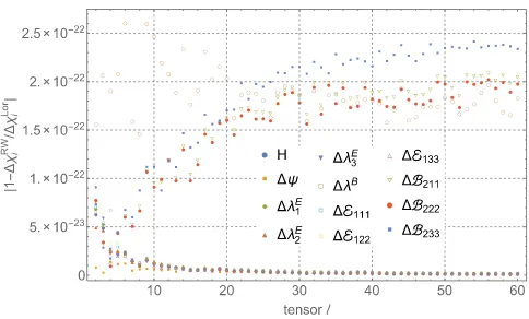
We have employed two independent calculations in the Regge-Wheeler and Lorenz gauges: see Sec.IIIor Ref.[60] for details, respectively. Both codes are implemented in Mathematica, which allows us to go beyond machine precision. We find that the Regge-Wheeler and Lorenz gauge results for retarded field contribution to the invariants agree to around 22–24 significant figures. This high level of

agreement, exemplified in Fig.1, increases our confidence in the validity of the numerical calculation.

In Table I we present sample numerical results for the three conservative electric-type invariants. TableIIprovides the results for the three dissipative electric-type invariants. As the computation of the latter does not involve a regularization step, the dissipative results are considerably more accurate than for the conservative results. Our numerical results for the three conservative and one dissipative magnetic-type invariants are presented in TableIII.

B. Post-Newtonian expansions

As outlined in Sec. III B, we have made a post-Newtonian calculation of the octupolar invariants using a method which builds upon the work of Ref. [43]. This method allows us to take the expansions to very high order. Results at 15th post-Newtonian order are available in an online repository [66]. Here, for brevity, we truncate the displayed results at a relatively low order:

FIG. 1 (color online). Comparison of numerical results com-puted in the RW and Lorenz gauges for a variety of conservative gauge invariant quantities, Δ_{χi, along a circular orbit at}

r0¼10M. We see 22–24 significant digits agreement in the

TABLE I. Sample numerical results for the conservative electric-type octupolar invariants.

rΩ=M ΔE111 ΔE122 ΔE133

4 −6.87640142×10−2 _{5.634572704×10}−2 _{1.24182872×10}−2

5 −1.3622429846×10−2 _{9.45418747546×10}−3 _{4.1682423703×10}−3

6 −5.61141083923×10−3

3.477232505498×10−3 _{2.13417833373×10}−3

7 −2.925643118454×10−3 _{1.701979164325×10}−3 _{1.223663954129×10}−3

8 −1.710986615756×10−3 _{9.592475191788×10}−4 _{7.517390965770×10}−4

9 −1.075500995896×10−3 _{5.890480037652×10}−4 _{4.864529921306×10}−4

10 −7.120764484958×10−4 ₃

.838876753995×10−4 ₃

.281887730964×10−4

12 −3.494517915911×10−4 _{1.847169590917×10}−4 _{1.647348324994×10}−4

14 −1.913146810405×10−4

9.995537359206×10−5 _{9.135930744843×10}−5

16 −1.133949991793×10−4 _{5.879346730837×10}−5 _{5.460153187097×10}−5

18 −7.141332604056×10−5 _{3.682750321689×10}−5 _{3.458582282367×10}−5

20 −4.718352028785×10−5 _{2.423514347706×10}−5 _{2.294837681079×10}−5

30 −9.514915883987×10−6 _{4.835793521499×10}−6 _{4.679122362488×10}−6

40 −3.040712519124×10−6 _{1.538289606495×10}−6 _{1.502422912629×10}−6

50 −1.252723439259×10−6 _{6.321181929625×10}−7 _{6.206052462967×10}−7

60 −6.064208487551×10−7 _{3.054930741569×10}−7 _{3.009277745982×10}−7

70 −3.282027079848×10−7 _{1.651475883984×10}−7 _{1.630551195863×10}−7

80 −1.927657419028×10−7 _{9.691577786310×10}−8 _{9.584996403967×10}−8

90 −1.205253640043×10−7 _{6.055682885677×10}−8 _{5.996853514753×10}−8

100 −7.917190975864×10−8 _{3.975890910078×10}−8 _{3.941300065787×10}−8

500 −1.277421047615×10−10 _{6.392477321681×10}−11 _{6.381733154472×10}−11

1000 −7.991970194046×10−12 _{3.997657790884×10}−12 _{3.994312403162×10}−12

5000 −1.279743808249×10−14 _{6.399252758926×10}−15 _{6.398185323566×10}−15

TABLE II. Sample numerical results for the dissipative electric-type octupolar invariants.

rΩ=M ΔE113 ΔE223 ΔE333

4 1.43018712098924×10−2 _{−6.81363125080514×10}−3 _{−7.48823995908726×10}−3

5 1.69051912392376×10−3

−6.68228419170062×10−4

−1.02229070475370×10−3

6 3.93615041880796×10−4 _{−1.40326772303052×10}−4 _{−2.53288269577744×10}−4

7 1.24851076918558×10−4

−4.16707182592131×10−5

−8.31803586593453×10−5

8 4.78575862364605×10−5

−1.52593581419753×10−5

−3.25982280944852×10−5

9 2.09252624095044×10−5 _{−6.45207930480653×10}−6 _{−1.44731831046978×10}−5

10 1.00921765694192×10−5

−3.03317966765418×10−6

−7.05899690176504×10−6

12 2.90853534249746×10−6 _{−8.42878520552755×10}−7

−2.06565682194470×10−6

14 1.02905687355232×10−6 _{−2.90962875240999×10}−7

−7.38093998311317×10−7

16 4.21307269886127×10−7 _{−1.17032511794287×10}−7 _{−3.04274758091840×10}−7

18 1.92451417988312×10−7

−5.27522804430828×10−8

−1.39699137545229×10−7

20 9.57423553217574×10−8 _{−2.59726822309717×10}−8 _{−6.97696730907857×10}−8

30 6.63075048503344×10−9

−1.74627612621227×10−9

−4.88447435882117×10−9

40 1.00806706036123×10−9 _{−2.61810134057605×10}−10 _{−7.46256926303620×10}−10

50 2.34720446527898×10−10

−6.04700459200130×10−11

−1.74250400607885×10−10

60 7.14698583248068×10−11 _{−1.83158348544703×10}−11 _{−5.31540234703365×10}−11

70 2.61736513652863×10−11

−6.68285229858544×10−12

−1.94907990667008×10−11

80 1.09692221205352×10−11

−2.79307929655166×10−12

−8.17614282398351×10−12

90 5.09523969822615×10−12 _{−1.29465822904663×10}−12 _{−3.80058146917952×10}−12

100 2.56663032262918×10−12

−6.51067248226772×10−13

−1.91556307440241×10−12

500 7.32252735609857×10−17 _{−1.83582572460285×10}−17 _{−5.48670163149571×10}−17

1000 8.09167955607435×10−19

−2.02577720909791×10−19

−6.06590234697644×10−19

ΔE_111¼−8y4

þ8y5

þ30y6_{− 1711}

6 − 4681

512 π 2

y7

þ

₁₃₆₀₉₉

400 − 6255 1024π

2₋2048 5 γ−

4096 5 log2−

1024 5 logy

y8

−

_1604627

630 −

6413231

49152 π

2₋159664 105 γ−

18416

5 log2þ 4374

7 log3− 79832

105 logy

y9₋219136 525 πy

19=2

þO_ðy10

Þ;

ð4:1_Þ

ΔE_122¼4y4₋7 3y

5_−9y6

þ

₁₃₆₉

8 − 9677 2048π

2

y7

þ

₁₂₁₃₆₉

7200 þ 265 192π

2

þ1024₅ γ_þ2048

5 log2þ 512

5 logy

y8

−

_132611239

120960 −

240298535 1179648 π

2

þ173416₃₁₅ γ_þ53416

35 log2− 2916

7 log3þ 86708

315 logy

y9

þ109568₅₂₅ πy19=2

þO_ðy10

Þ; _ð4:2_Þ

ΔE_133¼4y4₋17 3 y

5_−21y6

þ

₂₇₃₇

24 − 9047 2048π

2

y7₋

_2571151

7200 − 14525

3072 π

2₋1024 5 γ−

2048 5 log2−

512 5 logy

y8

þ

_62957089

17280 −

394216079

1179648 π

2₋305576 315 γ−

75496

35 log2þ 1458

7 log3− 152788

315 logy

y9

þ109568₅₂₅ πy19=2þO_ðy10

Þ; ð4:3Þ

TABLE III. Sample numerical results for the magnetic-type octupolar invariants.

rΩ=M ΔB211 ΔB222 ΔB233 ΔB123

4 −6.148298254370×10−2 _{5.070286329453×10}−2 _{1.078011924917×10}−2 _{1.07801192491724×10}−2 5 −9.558323357929×10−3 _{7.670992694990×10}−3 _{1.887330662938×10}−3 _{1.88733066293848×10}−3 6 −3.155936380263×10−3 _{2.476758241817×10}−3 _{6.791781384454×10}−4 _{6.79178138445361×10}−4 7 −1.397948966284×10−3 _{1.081923065789×10}−3 _{3.160259004949×10}−4 _{3.16025900494923×10}−4

8 −7.234703923371×10−4 ₅

.550936330078×10−4 ₁

.683767593293×10−4 ₁

.68376759329306×10−4 9 −4.130973443372×10−4 _{3.151840931693×10}−4 _{9.791325116795×10}−5 _{9.79132511679517×10}−5 10 −2.528015715619×10−4 _{1.921517184307×10}−4 _{6.064985313116×10}−5 _{6.06498531311616×10}−5

12 −1.095551773983×10−4 ₈

.288773695651×10−5 ₂

.666744044177×10−5 ₂

.66674404417714×10−5 14 −5.444485917231×10−5 _{4.108569884562×10}−5 _{1.335916032669×10}−5 _{1.33591603266878×10}−5 16 −2.980264003325×10−5 _{2.245424872606×10}−5 _{7.348391307187×10}−6 _{7.34839130718667×10}−6 18 −1.753993694654×10−5 _{1.320134773357×10}−5 _{4.338589212967×10}−6 _{4.33858921296681×10}−6 20 −1.092394842331×10−5 _{8.215915676267×10}−6 _{2.708032747040×10}−6 _{2.70803274704046×10}−6 30 −1.770249199828×10−6 _{1.329249843091×10}−6 _{4.409993567363×10}−7 ₄

.40999356736253×10−7 40 −4.868817160862×10−7 _{3.653967138885×10}−7 _{1.214850021976×10}−7 _{1.21485002197624×10}−7 50 −1.788310960062×10−7 _{1.341778109443×10}−7 ₄

.465328506186×10−8 ₄

.46532850618555×10−8 60 −7.887212354333×10−8 _{5.917061308384×10}−8 _{1.970151045949×10}−8 _{1.97015104594935×10}−8 70 −3.946891664217×10−8 _{2.960771807198×10}−8 _{9.861198570192×10}−9 _{9.86119857019213×10}−9 80 −2.166444813367×10−8 _{1.625085708368×10}−8 _{5.413591049991×10}−9 _{5.41359104999132×10}−9 90 −1.276212037585×10−8 _{9.572758888543×10}−9 _{3.189361487310×10}−9 _{3.18936148731046×10}−9 100 −7.948907544564×10−9 _{5.962268324527×10}−9 _{1.986639220037×10}−9 _{1.98663922003664×10}−9 500 −5.716760192009×10−12 _{4.287586670256×10}−12 _{1.429173521752×10}−12 _{1.42917352175245×10}−12 1000 −2.528141980419×10−13

1.896108307399×10−13

6.320336730204×10−14

ΔE_113¼128 5 y

13=2₋108 5 y

15=2_þ512 5 πy

8₋46978 105 y

17=2_þ3794 45 πy

9

þ₄₉₆₁₂₅8 ð107554351_þ8467200π2_{−25885440γ−51770880log2−12942720logy}

Þy19=2_þOðy10

Þ; ð4:4Þ

ΔE_223¼−32

5 y

13=2₋18 5 y

15=2₋128 5 πy

8

þ8276₁₀₅ y17=2₋15242 315 πy

9

− 1

496125ð152535527þ16934400π

2_−51770880

γ−103541760log2−25885440logy_Þy19=2

þO_ðy10

Þ;

ð4:5_Þ

ΔE_333¼−96

5 y 13=2

þ126₅ y15=2₋384 5 πy

8

þ38702₁₀₅ y17=2₋3772 105 πy

9

− 1

165375ð235966427þ16934400π

2_−51770880

γ−103541760log2−25885440logy_Þy19=2

þO_ðy10

Þ;

ð4:6_Þ

ΔB_123¼64 3 y

7

þ36₅ y8

þ256₃ πy17=2₋5347 15 y

9

þ2197₁₅ πy19=2

þ₁₁₀₂₅4 ð3475113_þ313600π2−958720γ−1917440log2−479360logy_Þy10₋10961 7 πy

21=2

þO_ðy11

Þ;

ð4:7_Þ

ΔB_211¼−8y9=2

þ16₃ y11=2_−20y13=2

þ

−677

2 þ 5101

512 π 2

y15=2

− 1

230400ð246270016−20642025π 2

þ94371840γ_þ188743680log2_þ47185920logy_Þy17=2

− 1

154828800ð417740314624−17848070625π

2_{−131939696640}

γ−390644367360log2

þ123619737600log3−65969848320logy_Þy19=2₋219136 525 πy

10

þO_ðy21=2

Þ; _ð4:8_Þ

ΔB_222¼6y9=2_−4y11=2_þ83 4 y

13=2_{þ 1069}

4 − 7809

1024π 2

y15=2

þ₂₀₄₈₀₀1 ð234195584−19194125π2

þ62914560γ_þ125829120log2_þ31457280logy_Þy17=2

þ_114688001 ð125170823168−11193257425π2−5923143680γ−19177144320log2

þ7166361600log3−2961571840logyÞy19=2þ54784₁₇₅ πy10

þO_ðy21=2

Þ; ð4:9Þ

ΔB_233¼2y9=2₋4 3y

11=2₋3 4y

13=2

þ

₂₈₅

4 − 2393 1024π

2

y15=2

− 1

1843200ð137600128−7610925π

2_{−188743680γ−377487360log2−94371840logy}

Þy17=2

− 1

309657600ð2544131596288−266521809225π 2

þ103954513920γ_þ263505838080log2

−53747712000log3_þ51977256960logy_Þy19=2

þ54784₅₂₅ πy10

þO_ðy21=2

Þ; _ð4:10_Þ

Figure 2 shows sample comparisons of our PN and numerical results. We observe that, as higher-order PN terms are included in the comparison, the agreement improves for all values of r0. For large orbital radii the comparison saturates at the level of our (smaller than machine precision) numerical round-off error. For strong-field orbits, the comparison allows us to estimate how well the PN series performs in this regime. At r0¼ 10M we typically find that the 15PN series recovers the first 7–8 significant digits of the numerical result. At the

innermost stable circular orbit, atr0¼6M, the 15PN series successfully recovers the first 3–4 significant figures. The

excellent agreement we observe between our PN and numerical calculations gives us further confidence in both sets of results.

C. Behavior near the light-ring

With our numerical codes we can calculate the behavior of the octupolar invariants as the orbit approaches the light-ring atr0¼3M. In general, the invariants will diverge as the light-ring is approached, and knowledge of the rate of divergence, along with our high-order PN results and our other numerical results, may be useful in performing global fits for the invariants across all orbital radii. Such fits find utility in EOB theory and already results for the redshift, spin precession and tidal invariants have been employed in EOB models[25–27]. In this section we discuss, and give results for, the rate of divergence of the invariants near the light-ring but stop short of making global fits for the invariants.

The main challenge in computing conservative invariants near the light-ring is the late onset of convergence of the mode-sum in this regime (see Ref.[25]for a discussion of this behavior). This necessitates computing a great deal more lm-modes; typically we set lmax¼130 for our

calculations in this regime. By comparison, for orbits with r0¼4M we use lmax¼80. Not only then do we need to

numerically compute an additional 8085 lm-modes, on top of the 3239 modes required to reach lmax¼80, but

these higherlm-modes are more challenging to calculate FIG. 2 (color online). Comparison of our numerical and PN results for (left)ΔE_{122and (right)}ΔB_{123. For each invariant we plot the} relative difference between the numerical data and successive truncations of the relevant PN series, i.e., in the legend“xPN”means we are comparing against the PN series with all terms up to and including (relative)xPN order. As successive PN terms are added the agreement between the PN series and the numerical results improves. For the conservative invariants, such asΔE₁₂₂, the agreement between the PN series and the numerical data saturates at a relative accuracy of 13–14 significant figures. For the dissipative invariants,

such asΔB₁₂₃, the comparison saturates at 21_–22 significant figures. This difference in accuracy in the numerical data stems from the requirement to regularize the conservative invariants whereas the dissipative invariants do not require regularization.

FIG. 3 (color online). Divergence of the conservative octupolar invariants as the orbital radius approaches the light-ring. The electric-type invariants, ΔE_111, ΔE_122,ΔE_{133, diverge as} z−5=2 where z¼1−3M=r0. Two of the magnetic-type invariants,