Analysis of an aggregation‐based algebraic two‐grid method for a rotated anisotropic diffusion problem

This is a repository copy of Analysis of an aggregation based algebraic two grid method ‐ ‐ for a rotated anisotropic diffusion problem.

White Rose Research Online URL for this paper: http://eprints.whiterose.ac.uk/137610/

Version: Accepted Version

Article:

Chen, M-H and Greenbaum, A (2015) Analysis of an aggregation based algebraic two grid‐ ‐ method for a rotated anisotropic diffusion problem. Numerical Linear Algebra with

Applications, 22 (4). pp. 681-701. ISSN 1070-5325 https://doi.org/10.1002/nla.1980

© 2015 John Wiley & Sons, Ltd. This is the peer reviewed version of the following article: Chen, M. H., and Greenbaum, A. (2015) Analysis of an aggregation based algebraic ‐ ‐ two grid method for a rotated anisotropic diffusion problem. Numer. Linear Algebra Appl., ‐ 22: 681–701, which has been published in final form at https://doi.org/10.1002/nla.1980. This article may be used for non-commercial purposes in accordance with Wiley Terms and Conditions for Self-Archiving. Uploaded in accordance with the publisher's

self-archiving policy.

[email protected] https://eprints.whiterose.ac.uk/

Reuse

Items deposited in White Rose Research Online are protected by copyright, with all rights reserved unless indicated otherwise. They may be downloaded and/or printed for private study, or other acts as permitted by national copyright laws. The publisher or other rights holders may allow further reproduction and re-use of the full text version. This is indicated by the licence information on the White Rose Research Online record for the item.

Takedown

If you consider content in White Rose Research Online to be in breach of UK law, please notify us by

Analysis of an Aggregation-Based Algebraic Two-grid

Method for a Rotated Anisotropic Diffusion Problem

Meng-Huo Chen

Anne Greenbaum

January 2, 2015

Abstract

A two-grid convergence analysis based on the paper [Algebraic analysis of aggregation-based multigrid, by A. Napov and Y. Notay, Numer. Lin. Alg. Appl. 18 (2011), pp. 539-564] is derived for various aggregation schemes applied to a finite element discretization of a rotated anisotropic diffusion equation. As ex-pected, it is shown that the best aggregation scheme is one in which aggregates are aligned with the anisotropy. In practice, however, this is not what automatic aggregation procedures do. We suggest approaches for determining appropriate aggregates based on eigenvectors associated with small eigenvalues of a block split-ting matrix, or based on minimizing a quantity related to the spectral radius of the iteration matrix.

1

Introduction

Recently aggregation-based algebraic multigrid methods with piecewise constant prolon-gation have received considerable attention. See, for instance, [8, 11]. Although these methods may require extra Krylov space iterations on coarse grids in order to perform well in a multigrid setting [14, 10], their relative simplicity compared to other algebraic multigrid methods gives them a number of advantages. They require less setup time than standard algebraic multigrid methods and maintain better sparsity in the “coarse grid” matrices. They also maintain other important properties of the original matrix such as the M-matrix property [6, Theorem 3.6].

In [9] a powerful method was derived for analyzing the convergence of two-grid ag-gregation methods based on the quality of individual aggregates. While the two-grid convergence rates do not carry over to the multigrid V-cycle, it was shown in [14, 10] that similar convergence rates could be obtained in a multigrid setting by replacing the V-cycle with a K-cycle. Hence the two-grid convergence analysis is still an important step in understanding the behavior of these methods.

∗_{University of Washington, Dept. of Applied Mathematics, Box 352420, Seattle, WA 98195. This}

work was supportedd in part by NSF grant DMS-1210886.

†_{University of Washington, Dept. of Applied Mathematics, Box 352420, Seattle, WA 98195. This}

In this paper we apply the analysis techniques in [9] to a finite element discretiza-tion of a rotated anisotropic diffusion equadiscretiza-tion with homogeneous Dirichlet boundary conditions:

−(ǫcos2θ+ sin2θ)∂

2_u

∂x2 −2(1−ǫ) cosθsinθ ∂2_u

∂x∂y −(cos

2_θ+ǫsin2_θ)∂2u

∂y2 =f,

on [0,1]×[0,1], u(x,0) =u(x,1) =y(0, y) =u(1, y) = 0. (1)

This corresponds to a problem of the form −ǫuξξ − uηη = f in a (ξ, η) coordinate system that can be obtained by rotating the (x, y) coordinate system through angle

θ. We will always assume that ǫ ∈ [0,1] since for ǫ > 1, equation (1) corresponds to

−uξξ−ǫ−1uηη =ǫ−1f, where the direction of stronger coupling is just rotated byπ/2. We will deal with anglesθ between−π/2 andπ/2. Problems of this sort can be a challenge for aggregation-based algebraic multigrid methods if the direction of anisotropy is not aligned with the grid lines. Numerical experiments for the special case θ = π/4 show that if the aggregates can be chosen to align with the direction of anisotropy, then grid-size independent andǫ-independent convergence rates can be obtained with a two-grid method. In this paper we use the analysis in [9] to prove this. We suggest two possible strategies for automatically recognizing such cases and assembling the correct aggregates. We demonstrate that these strategies can result in smaller spectral radii for the iteration matrix in a two-grid method and that they can also be effective in a true multigrid K-cycle setting.

Problems of this type have been studied elsewhere. Different coarsening strategies were proposed, for instance, in [3, 15]. The interplay between the relaxation method and the coarsening strategy has also been explored, for example, in [2, 7]. Most of this work has been in the context of classical algebraic multigrid (where restriction and prolonga-tion operators are more complicated) rather than aggregaprolonga-tion-based multigrid. In [16], a new “smoothed” aggregation approach was shown to yield mesh-size independent (or nearly independent) convergence rates for problems of the form (1), without changing the coarsening strategy. Here we work with the simplest, unsmoothed aggregation pro-cedure and try to determine if it can find aggregates for which even simple smoothers such as the damped Jacobi method can be effective. Another work that is closely related to ours is [4], where a different technique was used to show that if pairs of nodes were aggregated in or close to the direction of anisotropy, then if two of the three parameters – ǫ, θ, and the grid size – were held fixed, the convergence rate of a two-grid method using Richardson iteration as a smoother could be bounded independent of the third parameter.

2

Two-grid Convergence Analysis

prolongation matrixP by

P =



     

0m0 0m0 . . . 0m0

1m1

1m2 . ..

1m_NC 

     

,

where 1mj is a vector of 1’s whose length is the number mj of variables

correspond-ing to the jth aggregate. The top block row of 0’s corresponds to variables that are not involved in the aggregation procedure (because, for instance, their rows might be strongly diagonally dominant and hence they can be dealt with efficiently by a fine grid relaxation). If there are m0 such variables then

PNC

j=0mj =N. Note that geometrically

P corresponds to piecewise constant interpolation from the collection of aggregates to the collection of fine grid points. Define an NC by NC “coarse grid matrix” AC by

AC =PTAP.

Let M1 and M2 denote pre- and post-smoothing matrices. For example, with a weighted Jacobi method M1 = M2 = ω−1_{diag(A); with a symmetrized Gauss-Seidel}

method M1 =MT

2 = lower triangle(A). The solution procedure will be to first perform ν1 relaxation steps with splitting M1, so that, starting with x(k) _{≡ x}(k,0)_{, we obtain}

new approximations x(k,j) _{via x}(k,j) _=x(k,j−1)_+M−1

1 (b−Ax(k,j−1)), j = 1, . . . , ν1. The

error e(k,j) _{≡ A}−1_b−x(k,j) _{then satisfies e}(k,j) _{= (I − M}−1

1 A)e(k,j−1) so that e(k,ν1) =

(I−M₁−1A)ν1_e(k,0)_{. Next a “coarse grid correction” is performed: Restrict the residual}

r(k,ν1) ≡_b−_Ax(k,ν1)_{to the coarse grid by formingP}T_r(k,ν1)_{, solve forδin the linear system}

ACδ = PTr(k,ν1), form the longer vector P δ and add to x(k,ν1). The result is x(k,ν) =

x(k,ν1)_{+P A}−1

C PTr(k,ν1) so that the error now satisfies e(k,ν) = (I−P A−C1PTA)e(k,ν1) = (I−P A−_C1PT_A)(I−M−1

1 A)ν1e(k,0). Finally, perform ν2 post-smoothing steps using the

splitting M2 to obtain the new iterate x(k+1)_{. The resulting error is}

e(k+1) _=E

T Ge(k), ET G = (I −M2−1A)ν2(I −P A−C1PTA)(I−M −1

1 A)ν1. (2)

The matrix ET G is the two-grid iteration matrix.

The asymptotic convergence rate of the method is determined by the spectral radius

ρ(ET G). In general, this is not the relevant quantity for studying short-time behavior of the iteration (and, hopefully, short-time behavior is all that will be observed!). In some cases, however, the spectral radius also gives a measure of the amount by which the A-norm of the error is reduced at each step. The A-norm of a vector v is kvkA ≡

hAv, vi1/2 _{= kA}1/2_{vk, where k · k without a subscript denotes the 2-norm. From (2) it}

follows that A1/2_e(k+1) _=A1/2_E

T GA−1/2(A1/2e(k)) and hence

ke(k+1)kA ≤ kA1/2ET GA−1/2k · ke(k)kA.

The matrix A1/2_E

T GA−1/2 has the same eigenvalues as ET G so that if this matrix is symmetric then its norm is ρ(ET G). The matrix A1/2ET GA−1/2 can be written in the form

(I−A1/2M2−1A1/2)ν2(I−A1/2P A−C1PTA1/2)(I−A1/2M −1

Hence if ν1 =ν2 and M1 = M2T, then this matrix is symmetric and the A-norm of the

error is reduced at each step by at least the factor ρ(ET G). In this paper we will study the spectral radius ρ(ET G), whether or not these symmetry conditions hold, because that is the quantity that is analyzed in [9].

Let an N byN matrix X be defined by

I−X−1A= (I−M₁−1A)ν1_(I−M−1

2 A)ν2. (3)

For example, if one post-smoothing only is done so thatν1 = 0 andν2 = 1, thenX =M2. If one step of pre-smoothing and one of post-smoothing is done then ν1 =ν2 = 1 and

I−X−1A=I −M₁−1A−M₂−1A+M₁−1AM₂−1A,

so that X−1 _{= M}−1

1 + M

−1

2 − M

−1

1 AM

−1

2 = M

−1

1 (M2 +M1 −A)M

−1

2 . We always

assume that this matrix is invertible and, in fact, SPD. For example, if M1 is the lower

triangular part of the SPD matrix A and M2 is the upper triangular part (MT

1 ), then X =M2(diag(A))−1_M1.

Just as equation (2) involves the “coarse grid” approximation of the matrixA−1_A=I

through the termP A−_C1PT_{A, whereA}

C =PTAP, there will be other matrices for which this sort of term is relevant. For any N byN matrix Y, define

πY ≡P(PTY P)−1PTY ≡P YC−1PTY. (4)

The following theorem is proved in [9] and is a slight generalization of [5, Theorem 4.2]:

Theorem 3.1 (Napov and Notay [9]). LetA be an N by N SPD matrix and let P

be an N byNC matrix of rank NC < N. Let M1,ν1, M2,ν2 be such that X, defined in

(3), is SPD and let ET G be the two-grid iteration matrix defined in (2). Then

ρ(ET G)≤max

λmax(X−1A)−1, 1− 1

µX

, (5)

where λmax(·) denotes the (algebraically) largest eigenvalue, and

µX =λmax(A−1X(I−πX)).

Moreover, for any N byN SPD matrix D,

µX ≤λmax(D−1X)·µD, µD ≡λmax(A−1D(I−πD)). (6)

In particular, if M1 =M2 =ω−1_{D with ω}−1 _≥λ

max(D−1A), then

ρ(ET G) = 1− 1

µX

, (7)

and µX ≤ω−1µD, with equality if ν1+ν2 = 1.

bound (6) on µX is just ω−1. The second, µD = λmax(A−1D(I −πD)) gives a measure of how effectively eigenvectors associated with the large eigenvalues ofA−1 _{are damped}

by the coarse grid correction. If ν1 = ν2 = 1, then X = ω−1_{D(2D− ωA)}−1_{D and} λmax(D−1X) = ω−1λmax((2D−ωA)−1D). Typically, the matrix 2D−ωA is strongly diagonally dominant so that it is easy to estimateλmax(D−1X). For example, ifAhas 2’s on its main diagonal and −1’s on the first sub- and super-diagonal, as in a 1D problem for the Laplacian, thenD= 2I,λmax(D−1A)<2, soω−1 = 2 is a reasonable choice, and then the matrix 2D−ωA has 3’s on its main diagonal and 1/2’s on the first sub- and super-diagonal. Hence by Gerschgorin’s theorem the smallest eigenvalue of this matrix is greater than or equal to 2; that is the largest eigenvalue of the inverse matrix is less than or equal to 1/2, and the bound onλmax(D−1X) is ω−1 = 2.

In general, it seems difficult to determine the quantity µD on the right-hand side of (6), so it is not clear that this theorem has helped much in the goal of estimating the spectral radius ρ(ET G). However, the next theorem in [9] explains how to estimate the quantity µD by studying the individual aggregates.

Assume that A can be written in the form A=Ab +Ar, where Ab and Ar are both symmetric and nonnegative definite and Ab is block diagonal, with blocksizes equal to the corresponding aggregate size:

Ab =

     A(0) A(1) . ..

A(NC)

     , (8)

where A(k)_{, k = 0,1, . . . , N}

C, is of size mk by mk.

If the matrix A is diagonally dominant, then one way to create this splitting is to take the diagonal blocks of Ab to be the corresponding diagonal blocks of A, with the sum of absolute values of the remaining entries in each row or column of A subtracted from the corresponding diagonal entry of Ab. For example, if

A=        

2 −1

−1 2 −1

−1 2 −1

−1 2 −1

−1 2 −1

−1 2

        (9)

and successive pairwise aggregation is used, then a possible choice for Ab and Ar is

Ab =

           

2 −1 | |

−1 1 | |

− − | − − | − −

| 1 −1 |

| −1 1 |

− − | − − | − −

| | 1 −1

| | −1 2

           

, Ar =

            | |

1 | −1 |

− − | − − | − −

−1 | 1 |

| 1 | −1

− − | − − | − −

| −1 | 1

In this way, bothAb andAr are weakly diagonally dominant, hence nonnegative definite. If we choose to omit the first and last variables from the aggregation procedure and reorder rows and columns so that these two variables are first, followed by variables 2 and 3 and then 4 and 5, the matrixA takes the form

A=        

2 0 −1 0 0 0 0 2 0 0 0 −1

−1 0 2 −1 0 0

0 0 −1 2 −1 0 0 0 0 −1 2 −1 0 −1 0 0 −1 2

        .

and we can split this as

Ab =

           

1 | |

1 | |

− − | − − | − −

| 1 −1 |

| −1 1 |

− − | − − | − −

| | 1 −1

| | −1 1

           

, Ar =

           

1 | −1 |

1 | | −1

− − | − − | − −

−1 | 1 |

| 1 | −1

− − | − − | − −

| −1 | 1

−1 | | 1

            .

Other such splittings are possible as well. In Section 4 we describe a splitting that is appropriate for finite element discretizations, even when the matrix is not diagonally dominant. Once the splitting is set, the following theorem from [9] enables one to estimate the ‘global’ parameter µD in (6) by ‘local’ quantities µ(Dk) associated with each aggregate k.

Theorem 3.2 (Napov and Notay [9]). Using the notation of Theorem 3.1, let

A=Ab+Arbe a splitting of the SPD matrixAsuch thatAbandArare both nonnegative definite and Ab has the form (8). Assume that D in Theorem 3.1 also has the block diagonal form: D=      D(0) D(1) . ..

D(NC)

     ,

where each block D(k) _{is m}

k bymk, k= 0, . . . , NC. Define

µ(0)_D =

0 if m0 = 0

sup_v∈Rm_0\N(A(0)₎v

T_D(0)_v

vT_A(0)_v if m0 >0

,

and for k = 1, . . . , NC,

µ(_Dk)= (

0 if mk = 1

sup_v∈Rmk_\N(A(k)₎

vT_D(k)_(I−π(k)

D )v

vT_A(k)_v if mk >1

where

π(_Dk) =p(k)(p(k)TD(k)p(k))−1p(k)TD(k),

and p(k) _{is the vector of 1’s in column k of P. Then}

µD ≤ max

k=0,...,NC

µ(_Dk).

Note that ifmk>1 thenN(A(k)) must be a subset ofN(D(k)(I−π(_Dk))) = span{p(k)}, in order for this theorem to give useful information. Otherwise µ(_Dk) = ∞ in (11). If

N(A(k)_{) is a subset of span{p}(k)_{}, then expression (11) can be replaced by}

µ(_Dk)= (

0 if mk = 1

sup_v∈R(A(k)_)\{0} v

T_D(k)_(I−π(k)

D )v

vT_A(k)_v if mk >1

, (12)

In example (9-10), taking D= 2I and each p(k)_{= (1,1)}T_{, we find}

π_D(k) = 1 2

1 1 1 1

, k = 1,2,3,

so that

D(k)(I −π_D(k)) =

1 −1

−1 1

, k = 1,2,3.

Fork = 1, A(1) _{is nonsingular, so µ}(1)

D is the largest eigenvalue of A(1) −1

(D(1)_(I−π(1)

D )), which is easily seen to be

λmax "

2 −1

−1 1

−1

1 −1

−1 1

# = 1.

Similarly, µ(3)_D = 1. For k = 2, A(2) _{is singular but its null space is the span of p}(2) _and

its range is the span of (1,−1)T_{. In fact A}(2) _{= D}(2)_{(I −π}(2)

D ), so it is clear that the quantity in (12) is again 1. Thus in this example the bound from Theorem 3.2 isµD ≤1. Combining this with the bound on λmax(D−1X) when ν1 +ν2 = 1 or ν1 = ν2 = 1, we

obtain the estimate µX ≤2. Hence from Theorem 3.1,

ρ(ET G)≤ 1 2.

In (9-10), we tookAto be a 6 by 6 matrix, but if we made it much larger, the blocks not connected to the two end points would be identical to A(2)_{, so the theorems would}

3

Finite Element Discretization

Problem (1) can be solved using a piecewise bilinear finite element approximation on a square grid with uniform spacing h in each direction. Letting

a = ǫcos2θ+ sin2θ b = (1−ǫ) cosθsinθ c = cos2θ+ǫsin2θ,

equation (1) can be written in the form

−∇ ·

a b b c

∇u=f.

Letting φj(x, y) denote the standard bilinear basis function with value 1 at node j and 0 at all other nodes, and writing the approximate solution u(x, y) as PN

j=1ujφj(x, y), the coefficients uj can be determined by solving the equations

−

N X

j=1 uj

Z 1

0

Z 1

0

(∇φi)·

a b b c

∇φj

dx dy=

Z 1

0

Z 1

0

f φidx dy, i= 1, . . . , N.

The global stiffness matrix can be assembled from individual element matrices, which have the form

1 6



  

2a+ 3b+ 2c −2a+c a−2c −a−3b−c

−2a+c 2a−3b+ 2c −a+ 3b−c a−2c

a−2c −a+ 3b−c 2a−3b+ 2c −2a+c

−a−3b−c a−2c −2a+c 2a+ 3b+ 2c



  

.

When these are assembled into a global stiffness matrix (and multiplied by 6), the stencil of the finite element discretization becomes





−a+ 3b−c 2(a−2c) −a−3b−c

2(−2a+c) 8(a+c) 2(−2a+c)

−a−3b−c 2(a−2c) −a+ 3b−c



. (13)

Forθ =π/4, for example, the stencil is





1 2 −

5

2ǫ −1−ǫ − 5 2 +

1 2ǫ

−1−ǫ 8 + 8ǫ −1−ǫ

−5

2 + 1

2ǫ −1−ǫ 1 2 −

5 2ǫ



. (14)

4

The Matrix Splitting

Figure 1: Potential aggregates on a grid of 22×22 interior nodes.

The nodes that arenotincluded in a potential aggregate are ones whose rows are strongly diagonally dominant because they couple to Dirichlet boundary points; these make up the blockA(0)_{. The other blocks inA}

b are then 16×16. Element matrices corresponding to each of the nine elements in the potential aggregate will be assembled to form a block of Ab, and the remaining element matrices will be assembled to form Ar. Since each of the element matrices is nonnegative definite, the matrices Ab and Ar will be as well. Note that each block of Ab (except A(0)) is the finite element discretization of a Neumann problem on the potential aggregate, hence has null space consisting of the constant vectors (assuming 0 < ǫ ≤ 1 in (1)). Note also that if ǫ = 0 in (1) then this actually corresponds to a 1D problem: uηη = f. A vector that represents a function u that satisfies uηη = 0 and is constant in the ξ direction will also lie in the null space of

A(k)_{, and whenǫ >0 is small, this will be a near null vector for A}(k)_.

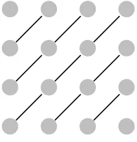
Actual aggregates will be formed from subsets of the nodes in the potential aggre-gates. For example, when θ =π/4, it is reasonable to aggregate points along diagonal lines, as pictured in Figure 2.

Figure 2: Diagonal aggregates.

This means that the structure is slightly different from that described in [9], where it was assumed that the aggregate size was the same as the block size in Ab.

then along the diagonals two spaces below and above the main one, etc., then the transpose of the block of P corresponding to thekth potential aggregate is

P(k)T =          

1 1 1 1

1 1 1

1 1 1 1 1 1 1 1 1           (15)

Thus each P(k) _{is a 16 by 7 matrix andπ}(k)

D is a 16 by 16 matrix. The block size in Ab is 16 by 16, but the individual aggregate sizes range from 1 to 4. This requires a minor change in the statement of Theorem 3.2.

Theorem 3.2’. Using the notation of Theorem 3.1, let A = Ab+Ar be a splitting of the SPD matrix A such that Ab and Ar are both nonnegative definite and Ab has the form

Ab =

     A(0) A(1) . ..

A(Nb)

     ,

where each block A(k) _{is s}

k by sk, k = 0, . . . , Nb. Assume that D in Theorem 3.1 also

has the block diagonal form

D=      D(0) D(1) . ..

D(Nb)

     ,

where each block is sk bysk. Define

µ(0)_D =

_{0 if s}

0 = 0

sup_v∈Rs_0\N(A(0)₎v

T_D(0)_v

vT_A(0)_v if s0 >0

, (16)

and for k = 1, . . . , Nb,

µ(_Dk) = (

0 if sk = 1

sup_v∈Rsk_\N(A(k)₎

vT_D(k)_(I−π(k)

D )v

vT_A(k)_v if sk >1

, (17)

where

π_D(k) =P(k)(P(k)TD(k)P(k))−1P(k)TD(k),

and P(k) _{represents the block of P corresponding to the kth potential aggregate. Then}

µD ≤ max

k=0,...,Nb

In order for this theorem to give useful information when somesk >1,k = 1, . . . , Nb, the null space of A(k) _{must be a subset of the null space of D}(k)_{(I −π}(k)

D ); otherwise

µ(_Dk) = ∞ in (17). The proof of this slightly generalized theorem is almost identical to the one in [9]. We include it here because it shows where an overestimate of µD can occur when a block A(k) _{has a near null vector that is not a near null vector of} D(k)_{(I − π}(k)

D ), which is often the case when the anisotropy in problem (1) is large and aggregates cannot be perfectly aligned with the direction of anisotropy. For such problems, aligning aggregates close to the direction of anisotropy may yield better results than the theorem predicts.

Proof of theorem: Assume wlog that each µ(_Dk) < ∞, k = 0,1, . . . , Nb; otherwise the result is trivial. Ifs0 >0 then this implies thatA(0) _{is positive definite so the expression}

for µ(0)_D becomes

µ(0)_D =

0 if s0 = 0

sup_v6=0 v

T_D(0)_v

vT_A(0)_v if s0 >0

.

To establish (18), first note that

D(I−πD) = 

   

D(0)

D(1)_(I−π(1)

D ) . ..

D(Nb)(I−π(Nb)

D )



   

.

Hence expression (6) for µD can be written as

µD = λmax(A−1D(I−πD)) = max

v∈RN

v6=0

vT_D(I−π D)v

vT_Av

= max v6=0

vT_D(I−π D)v

vT_A

bv+vTArv

= max v6=0

v(0)T_D(0)_v(0)₊PNb

k=1v(k)

T

D(k)_{(I −π}(k)

D )v(k) PNb

k=0v(k)

T

A(k)_v(k)_+vT_A rv

, (19)

where we have writtenv in the block form v = (v(0)T, v(1)T, . . . , v(Nb)T₎T_.

Let w = (w(0)T_{, w}(1)T_{, . . . , w}(Nb)T)T be a vector that attains the maximum in (19).

First note that if each termw(k)T_A(k)_w(k)_{,k = 0,1, . . . , N}

bin the sum in the denominator of (19) were 0, then the numerator of (19) would also be 0 since each µ(_Dk) is finite. If this were the case, then since A is SPD, the other term in the denominator, wT_A

rw, would have to be positive and then µD = 0. In this case, the result (18) holds trivially. Therefore we can assume that at least one of the terms w(k)T_A(k)_w(k) _{is nonzero and,}

since each A(k) _{is nonnegative definite, this implies that the sum in the denominator of}

(19) is positive. SinceAr is nonnegative definite we can write

µD ≤

w(0)T_D(0)_w(0)₊PNb

k=1w(k)

T

D(k)_(I−π(k)

D )w(k) PNb

k=0w(k)

T

Since the numerator and denominator each consist of a sum of nonnegative terms (or positive terms if we eliminate any zeros), the ratio of these sums is less than or equal to the largest ratio of the terms. [To see this, note that if a1, . . . , an, b1, . . . , bn > 0, then (Pn

i=1ai)/(Pin=1bi) = Pni=1(ai/bi)·(bi/Pnj=1bj), which is a convex combination of the ratiosai/bi, hence less than or equal to the maximum of these ratios.] Thus we can write

µD ≤ max

k=0,...,Nb

w(k)T_D(k)_(I−π(k)

D )w(k)

w(k)T_A(k)_w(k) (where π (0)

D ≡0) (21)

≤ max

k=0,...,Nb

sup v∈Rsk\N(A(k)₎

vT_D(k)_(I−π(k)

D )v

vT_A(k)_v (22)

= max k=0,...,Nb

µ(_Dk).

Note that in going from equality (19) to inequality (20), the term wT_A

rw was dropped; since Ar is small compared to Ab, this will not change the ratio much

un-less w is a near null vector of Ab. In addition to the upper bound (18), a lower bound on µD was derived in [9, Theorem 4.1]. Based on (19), one can give a lower bound on µD by inserting any nonzero vector into the expression on the right-hand side. The vector suggested in [9] was ˜v = (α0v∗(0)

T

, α1v(1)∗ T

, . . . , αNbv

(Nb)

∗ T

)T_{, where each v}(k) ∗ is a unit vector that achieves the supremum in (22), and

αk =γk(v(∗k) T

A(k)v∗(k))−1/2, k= 0,1, . . . , Nb, (23)

where theγk’s are parameters on the order of 1. Substituting ˜v into the right-hand side of (19), gives the lower bound

µD ≥

α2 0(v

(0)

∗ T

D(0)_v(0)

∗ ) +PN_k=1b α2k(v

(k)

∗ T

D(k)_(I−π(k)

D )v

(k)

∗ )

PNb

k=0α2k(v

(k)

∗ T

A(k)_v(k)

∗ ) + ˜vTAr˜v

=

PNb

k=0γk2µ

(k)

D PNb

k=0γk2+ ˜vTArv˜

. (24)

Unfortunately, this lower bound is not very useful in some of the numerical examples presented later because ˜vT_A

rv˜is large compared to the other term in the denominator.

5

Convergence Rates for Various Aggregates

step is performed at each iteration and also when just one pre- or one post-smoothing is performed. We consider both possibilities, using a damped Jacobi method with damping factor ω−1 _{satisfying the assumption needed for (7) in Theorem 3.1. By Gerschgorin’s}

theorem, using the stencil in (14), the eigenvalues ofD−1_{Aare at most (9 + 3ǫ)/(4 + 4ǫ)}

if ǫ≤ 1/5 or 2 if ǫ >1/5, so these will be the values used for ω−1_{. Thus D = diag(A)}

andD(k)_{,k = 1, . . . , N}

b, is the 16 by 16 block of Dcorresponding to potential aggregate

k: D(k) _{= 8(1 + ǫ)I}

16×16. We start with the diagonal aggregates pictured in Figure 2

and P(k) _{defined by (15).}

For problems with a fixed stencil such as that in (14) (i.e., the values in the stencil do not depend on the location within the domain) and potential aggregates as pictured in Figure 1 (where the number of interior nodes in each direction is 4m+ 2 for some integer

m so that each potential aggregate is 4 by 4), the blocks A(k) _{and D}(k)_{, k = 1, . . . , N}

b, in Theorem 3.2’ are all identical. Thus, except for the computation of µ(0)_D which is easily estimated with Gerschgorin’s theorem, the problem of bounding µD reduces to the problem of finding the largest (determined) generalized eigenvalue of a single pair of 16 by 16 matrices. [The fact that the expression on the right-hand side of (17) is a generalized eigenvalue follows from a generalization of the Courant-Fischer minimax theorem [1].]

For the problem with stencil (14) andP(k)_{defined by (15), one can look at the}

matri-cesA(k)_{and D}(k)_(I−π(k)

D ) symbolically and see that forǫ >0 the null space of A(k) con-sists of the constant vectors, while whenǫ= 0 the null space ofA(k)_{consists of linear}

com-binations of the constant vector and the vector (0,0,0,0,1,1,1,−1,−1,−1,2,2,−2,−2,3,−3)T (ordering nodes along the main diagonal of the potential aggregate first, then along the first upper and first lower diagonal, etc.). The null space of D(k)_(I−π(k)

D ) consists ofall vectors that are constant along diagonals and so contains each of these vectors.

Numerically computing generalized eigenvalues of a pair of singular matrices can be hazardous, but knowing the null spaces of the matrices involved makes this computation easy; it can be converted to a problem involving a positive definite matrixZ∗A(k)_{Z and}

the semidefinite matrixZ∗D(k)_(I−π(k)

D )Z whereZ has dimensionssk by rank(A(k)) and the columns of Z span the range of A(k) _{[1]. Figure 3 (a) shows a plot of µ}(k)

D vs ǫ. Using Gerschgorin’s theorem one can bound µ(0)_D based on the stencil (14). Since each node in A(0) _{couples to at least three boundary nodes, the smallest eigenvalue of} A(0) _{is at least}

8 + 8ǫ−

3 + 3ǫ+ 5 2−

1 2ǫ+

1 2 −

5 2ǫ

=

2 + 8ǫ if ǫ ≤1/5 3 + 3ǫ if ǫ >1/5 .

SinceD(0) _{= 8(1 +ǫ)I, the right-hand side of (16) is 8(1 +ǫ) over the smallest eigenvalue}

of A(0)_{; hence}

µ(0)_D ≤

(4 + 4ǫ)/(1 + 4ǫ) if ǫ≤1/5

8/3 if ǫ >1/5 .

a mesh size independent convergence rate for the 2-grid method with the aggregates shown in Figure 2.

0 0.1 0.2 0.3 0.4 0.5 0.6 0.7 0.8 0.9 1 3.5

4 4.5 5 5.5 6 6.5 7

epsilon

mu

D

(k)

(a)

0 0.1 0.2 0.3 0.4 0.5 0.6 0.7 0.8 0.9 1 0.5

0.6 0.7 0.8 0.9 1

epsilon

ρ

( E

TG

)

(b)

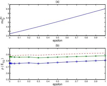
Figure 3: (a) µ(_Dk) for aggregates in Figure 2. (b) Bounds from Theorems 3.1 and 3.2’ on

ρ(ET G) (dashed) and actual values of ρ(ET G) on a 42 by 42 grid. Lower curve, marked with o’s, is for pre- and post-smoothing; upper curve, marked with∗’s, is for pre-smoothing only or post-smoothing only.

Unfortunately, the coarsening ratio for the aggregates shown in Figure 2 is only 7/16, while the coarse grid in a geometric multigrid method for a 2-D problem usually has about 1/4 as many points as the fine grid. The next aggregate type considered is shown in Figure 4. The potential aggregate is split into four smaller box-shaped aggregates so that the coarsening ratio is 1/4. This type of aggregate is standard for isotropic problems.

Figure 4: Box aggregates.

In this case, if nodes are again numbered consecutively in aggregates (so the lower left aggregate consists of nodes 1-4, the lower right aggregate consists of nodes 5-8, etc.) then the matrix D(k)(I−π(_Dk)) in (17) is

8(1 +ǫ)



  

I−



  

1 4e4eT4

1 4e4eT4

1 4e4eT4

1 4e4eT4



   

  

The constant vectors are contained in the null space of D(k)_{(I − π}(k)

D ), but note that when ǫ = 0 the null space of A(k) _{is not a subset of that of D}(k)_{(I − π}(k)

D ). The vector (0,0,0,0,1,1,1,−1,−1,−1,2,2,−2,−2,3,−3)T _{(using a diagonal ordering} of nodes), was shown to be in the null space of A(k), but with the current order-ing of nodes this vector becomes (0,1,−1,0,2,3,1,2,−2,−1,−3,−2,0,1,−1,0)T _and this is not in the null space of D(k)_{(I −π}(k)

D ) given above; the product is 2(1 + ǫ) · (0,4,−4,0,0,4,−4,0,0,4,−4,0,0,4,−4,0)T_{. Thus it can be expected that for small ǫ} the right-hand side of (17) will be large; µ(_Dk) approaches ∞ asǫ→0.

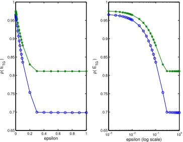
Figure 5 shows the spectral radius ρ(ET G) on a 42 by 42 grid using one pre- and one smoothing step per cycle (o’s) and using only one pre-smoothing or one post-smoothing step per cycle (∗’s). The left graph uses a linear scal in ǫ, while the right one displays the same results using a logarithmic scale for ǫ between 1.0e−3 and 1. The spectral radius is indeed close to 1 when ǫ is small, but it is not as bad as indicated by the upper bound in terms of µ(_Dk). For ǫ = 0.001, for example, the computed value of

µ(_Dk) was 595.12, while the value ofµD on the 42 by 42 grid was only 17.95. The spectral radius of the iteration matrix was 0.9655 for ν1 = ν2 = 1 and 0.9752 for ν1 +ν2 = 1, while the estimate based on µ(_Dk) would have been µX ≤(9.003/4.004)·595.12 = 1338.1,

ρ(ET G)≤1−1/1338.1 = 0.9993.

0 0.2 0.4 0.6 0.8 1 0.65

0.7 0.75 0.8 0.85 0.9 0.95 1

epsilon

ρ

( E

TG

)

10−3

10−2

10−1

100

0.65 0.7 0.75 0.8 0.85 0.9 0.95 1

epsilon (log scale)

ρ

( E

TG

)

Figure 5: Actual values (o’s and∗’s) forρ(ET G) with box aggregates on a 42 by 42 grid. Lower curve with o’s is for pre- and post-smoothing, upper curve with ∗’s is for pre-smoothing only or post-smoothing only.

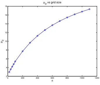
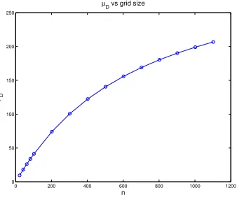
For these aggregates, when ǫ is small, the value µ(_Dk) is a large overestimate of µD, at least on a 42 by 42 grid. It is shown in Figure 6, however, that µD increases with the grid size. It is not clear whether it asymptotes to the value µ(_Dk) = 595.12 or to something smaller, but in either case it is large enough to indicate poor convergence of the two grid method. The lower bound (24) is not of much help here because the vectors v∗(k), k = 1, . . . , Nb used to derive that bound are near null vectors of A(k). This means that the coefficients α1, . . . , αNb in (23) will be huge if the γk’s are of order 1

and hence that ˜vT_A

rv˜ will be huge unless the γk’s can be chosen in such a way that

|v˜T_A

which case one obtains a lower bound on the order of µ(0)_D << µD.

0 200 400 600 800 1000 1200

0 50 100 150 200 250

n µD

µ_D vs grid size

Figure 6: Computed values ofµD vs grid sizenfor box aggregates,θ=π/4,ǫ= 0.001.

In general, whenD(k)_{is a scalar multiple of the identity, or, more generally, a diagonal}

matrix with positive diagonal entries, in order for a vector to be in the null space of

D(k)_{(I −π}(k)

D ), it must be constant on individual aggregates. But when ǫ = 0, the null space of A(k)_{contains a vector that is constant only on the diagonal aggregates pictured}

in Figure 2. Thus, for smallǫ, one can expect poor behavior (or at least a poor bound on the convergence rate) of the method for any aggregates other than those (or a refinement of those) shown in Figure 2.

The automatic aggregation procedure described in [10] and implemented in [13] does not use “potential aggregates” but tries various pairwise aggregations successively, in order to minimize a quantity related to the aggregate quality. For the problem with

θ = π/4 and ǫ = 0.001, in the first pass it formed pairwise aggregates aligned with the anisotropy, as pictured in Figure 7(a). On the second pass, however, the algorithm grouped pairs to the north and south above the 45◦ _{line and pairs to the east and west} below the 45◦ line, forming the parallelogram shaped aggregates shown in Figure 7(b). In this case, the spectral radius of the iteration matrix with pre- and post-smoothing on a 42 by 42 grid was 0.9307, indicating rather slow convergence of the two-grid method. This spectral radius increased to 0.9614 on an 82 by 82 grid, and while it will asymptote to something less than 1, the asymptotic value as N → ∞may be quite close to 1.

6

Determining Appropriate Aggregates

The negative results of the previous section suggest a possible way to determine which points to aggregate. Form the potential aggregates and the splitting Ab−Ar. Compute the eigensystem of each block A(k) _{and look at the eigenvectors corresponding to any}

small eigenvalues. Aggregate only points on which those eigenvectors are near constant. For example, when θ =π/6 and ǫ = 0.001, one finds that the matrix A(k) _{again has a}

(a) First pass

=⇒

(b) Second pass

Figure 7: First pass and second pass of the automatic aggregation procedure in [10]

twelfth components are close (−0.26 and −0.23), etc., with the close components lying along lines at an angleπ/6 with the vertical axis, as pictured in Figure 8. Additionally, components four and eight are fairly close (−0.46 and −0.35), as are components nine and thirteen (0.35 and 0.46), so these might be considered for aggregation as well.

Figure 8: Aggregates based on nearly equal components of eigenvector of A(k) _{corresponding}

to eigenvalue 0.0027 when θ=π/6,ǫ= 0.001.

Before proceeding with this example, it should be noted that with this parameter set, the finite element matrix defined by (13) is not an M-matrix; couplings to points to the left and right, (2−4ǫ) cos2_{θ + (2ǫ−4) sin}2_{θ = .4975, are positive. Hence not}

all points next to the boundary of the domain correspond to diagonally dominant rows, and such points should be included among the potential aggregates. In order to keep the blocks identical, we will now include all points next to the boundary among the potential aggregates. The number of interior grid points in each direction will be taken to be a multiple of 4 so that each blockA(k) _{still corresponds to a 4 by 4 group of nodes.}

Using the aggregates in Figure 8 does not result in a very small value for µ(_Dk) since the eigenvector of A(k) _{associated with the small eigenvalue is not extremely close to}

the null space of D(k)_{(I −π}(k)

D ); we found µ

(k)

0 200 400 600 800 1000 1200 2

4 6 8 10 12 14 16 18

n

µD

µ_D vs grid size

Figure 9: µD vs grid size nfor aggregates corresponding toθ=π/6;ǫ= 0.001.

Based on the above results it appears that eigenvectors corresponding to small eigen-values of A(k) _{do, indeed, indicate the direction of anisotropy and can be used to}

de-termine appropriate aggregates. However, to automate this procedure, one must define exactly what a “small” eigenvalue of A(k) _{is and how “nearly equal” eigenvector}

com-ponents must be in order to be aggregated. We will return to this later, but for now we consider another idea for automating the choice of aggregates. That is to try several different choices from among the potential aggregates and see which gives the smallest value for µ(_Dk). As noted previously, µD may be small even when µ(Dk) is not, but it is reasonable to expect that even when µ(_Dk) cannot be made small, aggregates that make it less large will be more likely to yield a good value for µD.

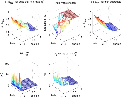
In the upper left block of Figure 11, we have plotted the spectral radius of the iteration matrix using pre- and post-smoothing on a 44 by 44 grid as a function of ǫ

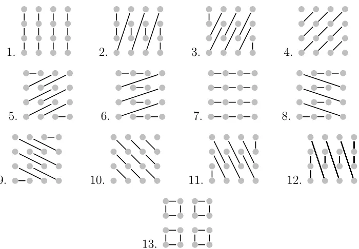
and θ, where the aggregates were chosen from among the 13 possible choices pictured in Figure 10. For these tests, we let ǫ range between 0 and 1; more specifically, ǫ = 0.001, 0.002, 0.005, 0.01, 0.02, 0.05, 0.1, 0.2, 0.3, . . . , 1. The angleθ ran from−π/2 toπ/2, in steps of 0.1.

Although some aggregate choices give a better coarsening ratio than others, we did not take this into account but simply chose the aggregate type that gave the smallest value forµ(_Dk). The upper middle block of Figure 11 shows the aggregate types that were chosen for each (ǫ, θ) pair. For ǫ > 0.5, box aggregates (type 13) were always chosen; these problems have only mild anisotropy. For more strongly anisotropic problems, the aggregates tended to align with the anisotropy, as can be seen by comparing the aggregate type numbers in Figure 11 with their definitions in Figure 10. Also plotted in Figure 11 are the values ofµ(_Dk) (lower left) and µD (lower right). It can be seen that the value of µD, which determines the spectral radius, is significantly less thanµ(Dk) for

ǫ near 0.

For comparison, the upper right plot in Figure 11 showsρ(ET G) using box aggregates only. It can be seen that for ǫ near 0, box aggregates give significantly larger values for

1. 2. 3. 4.

5. 6. 7. 8.

9. 10. 11. 12.

13.

Figure 10: Possible aggregate choices.

be well-represented in the potential aggregates, ρ(ET G) dropped as low as 0.7618 when appropriate aggregate types were chosen.

With information from these runs in hand, we decided to choose a definition of “small” eigenvalue and “nearly equal” components of the corresponding eigenvector and attempt to choose aggregates based on these notions, rather than having fixed aggregate choices. Recall that the difficulty with these problems stems from the fact that whenǫ= 0, each blockA(k) _{has a second null vector, in addition to the constant vector, and this}

will be a null vector ofD(k)_(I−π(k)

D )onlyif points within an aggregate correspond to equal components of this eigenvector. We decided that the second eigenvalue ofA(k) _{would be}

considered “small” if it was less than 1/2 times the next smallest eigenvalue. If it was greater than this, then we concluded that the problem was not highly anisotropic and chose box aggregates. If the second eigenvalue was deemed “small”, then we examined the corresponding eigenvector. We set a tolerance for “nearly equal” components at 0.05. We then looked for groups of four or more entries of the eigenvector whose values ranged over no more than three times the tolerance, or, 0.15. The largest such group was aggregated and we then checked the remaining entries for any more such groups, aggregating the largest such group and repeating until there were no more groups of four or more that differed by less than 0.15. We then searched the remaining entries for any groups of three whose values differed by at most twice the tolerance, or, 0.1. Such groups of three were aggregated. Finally we searched the remaining entries of the eigenvector for pairs that differed by no more than 0.05, and we aggregated such pairs. Remaining entries were left as singletons on the “coarse grid”.

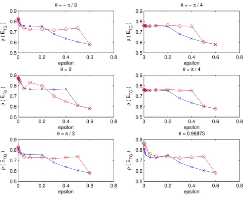
experiments, the results for negative θ were the same as for positive θ.] The spectral radius of the iteration matrix (with pre- and post-smoothing) using the newly chosen aggregates is plotted with x’s, while the spectral radius of the iteration matrix using aggregates chosen from the ones in Figure 10 is plotted with o’s. We went out only to

ǫ = 0.6, because for larger values of ǫ both codes chose box aggregates and thus had identical results. Forθ =±π/4, the new code chose the same diagonal aggregates (types 4 and 10) as the previous one. It got somewhat better results forǫ= 0.3 and 0.4 because it deemed the second eigenvalue not to be “small” in these cases and switched to box aggregates, while the code that based its choices on the minimum value of µ(_Dk) did not switch to box aggregates untilǫ= 0.5. Of course, this is very sensitive to the definition of a “small” second eigenvalue. For θ = 0 and ǫ small (less than 0.1) both codes chose vertical aggregates (type 1). The new code continued to choose vertical aggregates until it switched to box aggregates at ǫ = 0.5. Based on these results, it might have done better to switch earlier. The code that based its aggregate choice onµ(_Dk)chose aggregate type 12 when ǫ= 0.1 and aggregate type 2 when ǫ= 0.2 (near vertical aggregates), but these choices turned out not to be quite as good as the vertical aggregates. It switched to box aggregates when ǫ = 0.3 and got a smaller spectral radius than the new code until it too switched to box aggregates.

For θ = ±π/3 and θ = 0.99, the new code chose some aggregates that are not pictured in Figure 10. For example, whenθ =−π/3 andǫ≤0.1, it chose the aggregates below on the left (14), and for ǫ = 0.2 it chose the aggregates in the middle (15). It chose the aggregates on the right (16) when θ = 0.99 and ǫ ≤0.1. Here the coarsening ratio was only 10/16, and it might have been useful to force the code to aggregate some of the singletons. In general, however, both codes performed comparably, with similar coarsening ratios and with spectral radii between 0.5 and 0.9. The largest spectral radius still occurred for the smallest value of ǫ, namely, ǫ= 0.001 (unlessθ =±π/4), but both codes obtained significantly better results than using box aggregates for small values of

ǫ.

14. 15. 16.

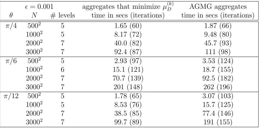
All of these results deal with a two-grid method and the spectral radius of the re-sulting iteration matrix. In practice, of course, more grid levels are used and the simple iteration procedure described here is usually accelerated using conjugate gradients or related iterative methods. To see if these two-grid results would carry over to a K-cycle multigrid method with flexible conjugate gradient acceleration, we decided to test the first aggregation strategy (based on minimizing µ(_Dk) using aggregate choices in Figure 10) in the code AGMG [10]. This aggregation strategy was used only on the finest level, where it was straightforward to identify the potential aggregates and then to choose the actual aggregates from among the choices in Figure 10 to minimize µ(_Dk). Aggregates at other levels were formed using the procedure in the AGMG code. Number of iterations and execution times were compared, with and without the new aggregation strategy, for

ǫ = 0.001 aggregates that minimize µ(_Dk) AGMG aggregates

θ N # levels time in secs (iterations) time in secs (iterations)

π/4 5002 _{5 1.65 (60) 1.87 (66)}

10002 _{5 8.17 (72) 9.48 (80)}

20002 _{7 40.0 (82) 45.7 (93)}

30002 _{7 92.4 (87) 111 (98)}

π/6 5002 _{5 2.93 (97) 3.53 (124)}

10002 _{6 15.1 (121) 18.7 (155)}

20002 _{7 70.7 (139) 92.5 (182)}

30002 _{7 201 (148) 262 (196)}

π/12 5002 _{5 1.78 (65) 3.07 (103)}

10002 _{5 8.53 (76) 15.7 (125)}

20002 _{7 38.5 (85) 77.4 (146)}

30002 _{7 99.7 (89) 191 (155)}

Table 1: Timing and iteration counts for ǫ = 0.001 with and without the new aggregation procedure on the finest grid.

with a zero initial guess. Results are shown in Table 1, where it can be seen that the new aggregation strategy for the finest level did, indeed, reduce both the number of iterations and the computation time. While more experiments are needed to determine if this approach is really a viable alternative – Can we identify potential aggregates without knowing the geometry of the problem? Can the new aggregation strategy be used effectively on other levels as well? – preliminary results look promising.

7

Conclusions

We have used the analysis in [9] to show that if diagonal aggregates are used in a two-grid aggregation method to solve a rotated anisotropic diffusion equation with angle of anisotropy θ = π/4, then one obtains a bound on the convergence rate that is inde-pendent of the mesh size and can be made indeinde-pendent of ǫ, the level of anisotropy, as well.

We have suggested two possible strategies for choosing appropriate aggregates, based on assembling groups of nodes that are candidates for aggregation, and then either choosing from a number of possible aggregates the one that minimizesµ(_Dk) or looking at the eigenvector corresponding to the smallest nonzero eigenvalue ofA(k) _{and aggregating}

aggregate choices. The increase in work for the second strategy would not be as great. The question of how to choose the “potential aggregates” has not been addressed in this paper. If the problem comes from a PDE (and this is known), then nodes that are geometrically close make appropriate potential aggregates. In an algebraic setting, such nodes might be identified using current methods of defining “strongly connected” points.

The spectral radii observed in this paper arenotspectacular in the realm of multigrid methods. Still, it should be remembered that the problems studied here are typically very difficult for algebraic multigrid methods and that the analysis was for the simplest possible outer iteration and the simplest smoother, damped Jacobi. Early experiments with the aggregation strategy in a true multigrid K-cycle using Gauss-Seidel smoothing look promising, but much remains to be done.

Acknowledgments: The authors thank Yvan Notay for helpful comments on a first draft of this paper, and they thank the referees for many additional helpful suggestions.

References

[1] H. Avron, E. Ng, and S. Toledo, A generalized Courant-Fischer minimax theorem, technical report LBNL-6393E, Lawrence Berkeley National Lab, August, 2008.

[2] A. Brandt,General hghly accurate algebraic coarsening, ETNA 10 (2000), pp. 1-20.

[3] J. Brannick, M. Brezina, S. MacLachlan, T. Manteuffel, and S. Ruge, An energy based AMG coarsening strategy, Numer. Lin. Alg. Appl., 13 (2006), pp. 133-148.

[4] J. Brannick, Y. Chen, and L. Zikatanov, An algebraic multilevel method for anisotropic elliptic equations based on subgraph matching, Numer. Lin. Alg. Appl. 19 (2012), pp. 279-295.

[5] R. Falgout, P. Vassilevski, and L. Zikatanov, On two-grid convergence estimates, Num. Lin. Alg. Appl., 12 (2005), pp. 471-494.

[6] H. Kim, J. Xu, and L. Zikatanov, A multigrid method based on graph matching for convection-diffusion equations, Num. Lin. Alg. Appl., 10 (2003), pp. 181-195

[7] O. Livne, Coarsening by compatible relaxation, Numer. Lin. Alg. Appl. 11 (2004), pp. 205-227.

[8] A. Muresan and Y. Notay, Analysis of aggregation-based multigrid, SIAM J. Sci. Comput. 30 (2008), pp. 1082-1103.

[9] A. Napov and Y. Notay, Algebraic analysis of aggregation-based multigrid, Numer. Lin. Alg. Appl., 18 (2011), pp. 539-564.

[11] Y. Notay, An aggregation based algebraic multigrid method, ETNA 37 (2010), pp. 123-146.

[12] Y. Notay, private communication.

[13] Y. Notay, AGMG: Iterative solution with AGgregation-based algebraic MultiGrid, http://homepages.ulb.ac.be/~ynotay/AGMG.

[14] Y. Notay and P. Vassilevski, Recursive Krylov-based multigrid cycles, Numer. Lin. Alg. Appl., 15 (2008), pp. 473-487.

[15] L. Olson, J. Schroder, R. Tuminaro, A new perspective on strength measures in algebraic multigrid, Numer. Lin. Alg. Appl., 17 (2010), pp. 713-733.

0

0.5 1

−2 0 2 0.4 0.6 0.8 1

epsilon

ρ ( E

TG ) for aggs that minimize µD (k)

theta

ρ

( E

TG

)

0

0.5 1

−2 0 2 0 5 10 15

epsilon Agg types chosen

theta

agg type 1−13

0

0.5 1

−2 0 2 0 50 100

epsilon Min µ

D (k)

theta

µ D

(k)

0

0.5 1

−2 0 2 0 5 10

epsilon

µ

D corres to min µD k)

theta

µ D

0

0.5 1

−2 0 2 0.4 0.6 0.8 1

epsilon

ρ ( E

TG ) for box aggregates

theta

ρ

( E

TG

)

Figure 11: Upper left: ρ(ET G) on a 44 by 44 grid using pre- and post-smoothing and aggregates that minimize µ(_Dk). Upper middle: Aggregate types (1-13) that were chosen. Upper right:

ρ(ET G) using box aggregates only. Lower left: µ(_Dk)is still fairly large forǫnear 0. Lower right:

0 0.2 0.4 0.6 0.8 0.5

0.6 0.7 0.8 0.9

epsilon

ρ

( E

TG

)

θ = − π / 3

0 0.2 0.4 0.6 0.8

0.5 0.6 0.7 0.8 0.9

epsilon

ρ

( E

TG

)

θ = − π / 4

0 0.2 0.4 0.6 0.8

0.5 0.6 0.7 0.8 0.9

epsilon

ρ

( E

TG

)

θ = 0

0 0.2 0.4 0.6 0.8

0.5 0.6 0.7 0.8 0.9

epsilon

ρ

( E

TG

)

θ = π / 4

0 0.2 0.4 0.6 0.8

0.5 0.6 0.7 0.8 0.9

epsilon

ρ

( E

TG

)

θ = π / 3

0 0.2 0.4 0.6 0.8

0.5 0.6 0.7 0.8 0.9

epsilon

ρ

( E

TG

)

θ = 0.98873

Figure 12: ρ(ET G) on a 44 by 44 grid using pre- and post-smoothing and aggregates chosen based on “nearly equal” components of the eigenvector corresponding to a “small” eigenvalue of A(k) _{(curve marked with x’s) and using aggregates chosen from among those in Figure 10}