and Evolution
.
White Rose Research Online URL for this paper:
http://eprints.whiterose.ac.uk/151026/
Version: Published Version
Article:
Constable, George William Albert orcid.org/0000-0001-9791-9571 and McKane, Alan J.
(2018) Exploiting Fast-Variables to Understand Population Dynamics and Evolution.
Journal of Statistical Physics. pp. 3-43. ISSN 1572-9613
https://doi.org/10.1007/s10955-017-1900-1
[email protected] https://eprints.whiterose.ac.uk/
Reuse
This article is distributed under the terms of the Creative Commons Attribution (CC BY) licence. This licence allows you to distribute, remix, tweak, and build upon the work, even commercially, as long as you credit the authors for the original work. More information and the full terms of the licence here:
https://creativecommons.org/licenses/
Takedown
If you consider content in White Rose Research Online to be in breach of UK law, please notify us by
https://doi.org/10.1007/s10955-017-1900-1
Exploiting Fast-Variables to Understand Population
Dynamics and Evolution
George W. A. Constable1
·Alan J. McKane2
Received: 14 July 2017 / Accepted: 11 October 2017 / Published online: 1 November 2017 © The Author(s) 2017. This article is an open access publication
Abstract We describe a continuous-time modelling framework for biological population dynamics that accounts for demographic noise. In the spirit of the methodology used by statistical physicists, transitions between the states of the system are caused by individual events while the dynamics are described in terms of the time-evolution of a probability density function. In general, the application of the diffusion approximation still leaves a description that is quite complex. However, in many biological applications one or more of the processes happen slowly relative to the system’s other processes, and the dynamics can be approximated as occurring within a slow low-dimensional subspace. We review these time-scale separation arguments and analyse the more simple stochastic dynamics that result in a number of cases. We stress that it is important to retain the demographic noise derived in this way, and emphasise this point by showing that it can alter the direction of selection compared to the prediction made from an analysis of the corresponding deterministic model.
Keywords Stochastic models·Population genetics·Time-scale separation·Effective models·Noise-induced selection·Population dynamics
1 Introduction
In a series of articles on biological evolution published in the Journal of Statistical Physics, it is natural to ask what expertise and insights statistical physicists can bring to the study of evolution, and in what way might their approach to the subject differ from biologists.
B
Alan J. McKaneGeorge W. A. Constable [email protected]
1 Department of Mathematical Sciences, University of Bath, Bath BA2 7AY, UK
2 Theoretical Physics Division, School of Physics and Astronomy, The University of Manchester,
If the subject is the one that will largely interest us in this paper—the study of evolution within the framework of population genetics—these questions are more easily answered. This is because in a system containing a large, but finite, number of individuals with given genetic characteristics, genetic drift leads to a stochastic dynamics which has many of the features which allow the application of the ideas and techniques of non-equilibrium statistical physics. We will use this formalism, but in addition our approach will have parallels with the traditional methodology of theoretical physicists.
Firstly, we will stress the fundamental nature of the microscopic description. That is, we will start with genes as basic constituents, which can be in different states according to their type (allele), location (if the individual carrying the gene is located on an island), the sex of the individual carrying the gene, etc.
Secondly, since the microscopic description contains too much detail which is irrelevant at the macroscale (or in our case, the mesoscale, where some stochastic element is retained) we will derive areduced oreffectivemodel which contains parameters which depend on the parameters of the microscopic description and so encapsulate the relevant aspects of the microscopic description.
Thirdly, we will be interested ingenericbehaviour. By this we mean that we will attempt to formulate a microscopic description that does not have inbuilt assumptions that make the model more easily solvable. Instead we will try to formulate the model in such a way that it could be generalised to include many more effects, without changing its structure. In this philosophy, the simplifying assumptions are brought in during the process of obtaining the effective model, and should be clearly stated.
Finally, although the whole basis of our work is mathematical, we will use intuition to explore the admissibility of the techniques we use outside of their regime of strict applicability, and check their correctness through the use of computer simulations.
Although these ideas are familiar to the theoretical physics community, they tend to be utilised less in the biological sciences. For example, many biologists may use quite complex verbal arguments to gain insights. Conversely, our methodology may differ from that of many mathematical biologists, since rigorous justification will not be a central feature of our approach. In addition, many mathematical biologists are focussed on the deterministic dynamics found at the macroscale. Nevertheless, we view the approach we will discuss here as able to form a bridge between the intuition gleaned by biologists and the more analytic investigations of mathematicians. In this way we hope that our methods prove of interest to a wider audience outside of the theoretical physics community.
In a previous paper [43], we have reviewed the process of setting-up a description of this class of biological systems in terms of its basic constituents, and from this deriving the mesoscopic equations governing the dynamics which generalise what might be the more familiar macroscopic equations. In particular, in Ref. [43], we give formulae for writing down the form of the mesoscopic dynamics in terms of quantities which appear in the microscopic formulation. This essentially is the first point of our methodology described above, and so while we will discuss it here, we will refer the reader to this earlier paper for more details. Instead we will focus on the second point above, namely obtaining an effective theory that is more amenable to analysis than the original.
macro-scopic dynamics with a few long-lasting variables. Although this dynamics is macromacro-scopic, a mesoscopic extension can also be derived along the same lines [23]. In the theory of dynam-ical systems, the concept of a centre manifold (CM) is another manifestation of these ideas. During our discussion of this methodology, there will be several illustrations of the third and fourth points discussed above, namely the wish to use generic structures and the use of numerical simulations to check the precision of the approximations we utilise.
As we have already mentioned, one of our aims in writing this article is to make the ideas and techniques available to a larger audience. To help to achieve this we will present an application of the method in a pedagogical manner in Sect.2. We have chosen one of the simplest possible systems: haploid individuals on one of two islands of equal size which can migrate from one island to the other. It will be assumed that are only two possible alleles which are modelled by a Moran process. After this informal, and hopefully easily accessible, introduction to the method, we will describe its application to a number of models in Sect.3. These include: a haploid Moran model on an arbitrary number of islands with selection and mutation; a stochastic Lotka–Volterra competition model with an arbitrary number of islands and a stochastic Lotka–Volterra competition model with an arbitrary number of species; a derivation of the Hardy–Weinberg approximation from first principles; a model of epidemic spread on a network. In Sect.4, we will illustrate the method in the slightly more technical case where noise-induced dynamics are present. We will see that noise-induced selection can cause selection for genotypes that are neutral in a deterministic setting, and that further, this noise induced selection can, under certain conditions, be strong enough to reverse the direction of deterministic selection. We will illustrate this behaviour with reference to Lotka–Volterra competition models, where we will see that this effect can help alleviate the dilemma of cooperation, and a model of transitions between sex-chromosome systems. Finally, in Sect.5
we conclude with a discussion.
2 Pedagogical Example
In this section we will explain as simply as possible how to apply the ideas discussed in the Introduction to a concrete example. The example we choose is a Moran model with migration. We ask how this can be reduced to an effective one-island model.
2.1 Setting-Up the Model
We set up the model at the microscale, that is, at the level of haploid individuals who each carry an allele of type 1 or of type 2. The individuals can reside on one of two islands, both of which can only carry a fixed number of individuals, which we denote byN. We therefore denote byn1the number of individuals carrying allele 1 on island 1, byN−n1the number
of individuals carrying allele 2 on island 1, byn2the number of individuals carrying allele
1 on island 2, and byN −n2the number of individuals carrying allele 2 on island 2. So the
state of the whole system is given by only two variables, which we can form into the two-dimensional vectorn=(n1,n2). We would like to reduce this description to one involving
only one variable, which gives the fraction of individuals in the system carrying allele 1. This would allow us to calculate, for example, the probability that allele 1 or allele 2 fix, and the mean time to fixation.
0.0 0.2 0.4 0.6 0.8 1.0 0.0
0.2 0.4 0.6 0.8 1.0
x1
x2
0 500 1000 1500 2000 0.0
0.2 0.4 0.6 0.8
0 10
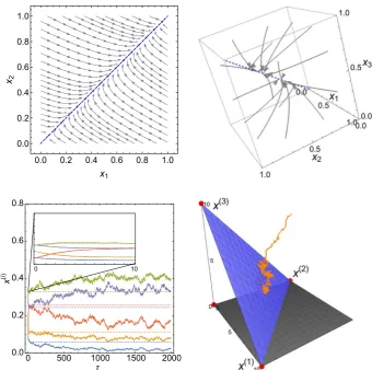
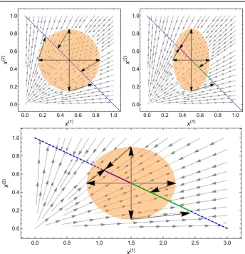
Fig. 1 Illustration of four systems featuring timescale separation that can be analysed with the methods reviewed in this paper. Top left panel: Phase plot for a haploid Moran model with two alleles on two islands with strong migration (described in Sect.2). The deterministic dynamics rapidly collapse to a slow subspace, indicated here by the blue dashed line. Top right panel: Deterministic trajectories (grey arrows) for a system similar to that in the top left panel but with three islands, addressed in Sect.3.1. Again, the deterministic dynamics rapidly collapse to a one-dimensional subspace indicated by the blue dashed line. Bottom left panel: Genotype frequencies as a function of time for a population genetic model, described in Sect.4.2. Stochastic trajectories (solid lines) initially rapidly relax on quasi-deterministic trajectories (inset) before reaching a one-dimensional slow subspace along which the system moves on a slower timescale. Bottom Right panel: A neutral three-species Lotka–Volterra model, addressed in Sect.3.2.2. Stochastic trajectories (orange) rapidly collapse along quasi-deterministic trajectories onto a two-dimensional slow subspace (blue surface), about which they are confined (Color figure online)
vectorn, to a new staten′. We write these transition rates asT(n′|n), with the initial state on the right and the final state on the left (some authors use the reverse convention). The probability distribution function (pdf) of the system, p(n,t), is then given by the master equation
dp(n,t)
dt =
n′=n
[image:5.439.49.390.51.389.2]This is relatively easy to understand. The first term on the right-hand side is made up of the probability of being in staten′multiplied by the probability of being in that state and making a transition to staten. It therefore represents the probability of starting in staten′and making a transition to staten. In the same way the second term on the right-hand side represents the probability of starting in statenand making a transition to staten′. Their difference, summed over all statesn′, different ton, gives the rate of increase ofp(n,t)with time.
The form we take for theT(n′|n)depends on the model choice. Here we choose the Moran model, because it is simple: it amalgamates births and deaths and asks that birth, death and migration events happen in such a way that the population size of each island,N, is kept fixed. These are not the most realistic assumptions, and we discuss ways to relax them later in the paper, but they have the merit that the number of model parameters is kept to a minimum. The method of constructingT(n′|n)also seems a little more complicated, due to the requirement of keeping a fixed number of individuals on each island. This is done as follows:
(i) Pick an island (with probability 1/2, since the islands are identical) and then pick an individual randomly from that island. Allow the individual to reproduce by duplicating the individual.
(ii) With probabilitym, the progeny migrates to the other island. In this case choose an individual on the other island at random to die.
(iii) With probability(1−m), the progeny remains on the same island. In this case choose an individual on the same island at random to die.
It should be noticed that the processes of birth and death are inextricably linked and that they are assumed to happen at rate 1, this choice being possible through a choice of time units. On top of this process, migration is imposed with a probability of occurrence equal to
m(0≤m≤1).
Following these rules, if the model is neutral the transition rate from the state(n1,n2)to
the state(n1+1,n2)is
T(n1+1,n2|n1,n2)=
1 2(1−m)
n1 N
(N−n1)
N +
1 2m
n2 N
(N−n1)
N . (2)
Similar expressions can be be found forT(n1−1,n2|n1,n2)and forT(n1,n2±1|n1,n2).
However, we would like to include selection in the model. In this case we have to weight the choice of picking an allele by the relative fitness of that allele on a particular island. Since we are aiming to be as simple as possible to illustrate the basic ideas, we will assume that this fitness weighting is the same on both islands, though it is simple enough to relax this condition. Therefore we will denote the fitness weighting of allele 1 to beW(1)(n)and of allele 2 to beW(2)(n). Then the four transition rates from state(n1,n2)to the new state are
T(n1+1,n2|n1,n2)=
1
2 (1−m)
W(1)(n)n1
W1(n)
(N−n1) N
+1
2m
W(1)(n)n2
W2(n)
(N−n1)
N ,
T(n1−1,n2|n1,n2)=
1
2 (1−m)
W(2)(n)(N−n1)
W1(n) n1 N
+1
2m
W(2)(n)(N−n2)
W2(n)
n1 N,
T(n1,n2+1|n1,n2)=
1
2 (1−m)
W(1)(n)n2
W2(n)
+1
2m
W(1)(n)n1
W1(n)
(N−n2)
N ,
T(n1,n2−1|n1,n2)=
1
2 (1−m)
W(2)(n)(N−n2)
W2(n) n2 N
+1
2m
W(2)(n)(N−n1)
W1(n)
n2
N, (3)
whereWi(n)=W(1)(n)ni+W(2)(n)(N−ni),i =1,2, is the fitness of the individuals on islandi. Here superscripts are a label for the two different alleles, whereas subscripts are a label for the two different islands. For further background on how to arrive precisely at the forms given by Eq. (3) the reader is referred to previous discussions in the literature [1,6,43]. If W(1) and W(2) are independent of n, then the selection is known as frequency independent selection. This will be assumed in this pedagogical treatment, and we write
W(1) = 1+α(1)s+O(s2)andW(2) = 1+α(2)s+O(s2), wheresis a selection coeffi-cient andα(1), α(2)are constants. Sincesis typically very small, we do not expect it will be necessary to include the orders2terms in the expressions forW(1)andW(2).
Equations (1) and (3) define the microscopic model, and once an initial conditionp(n,0)
for the pdf has been given, specify the dynamics for allt. All other systems discussed in this paper will have a similar structure; the form of the transition rates will differ depending on the system, but in all cases the substitution of these rates into the master equation (1) will give the dynamics. As we discussed in the Introduction, the validity of our methods and approximations are checked via computer simulations, and these use the microscopic model defined by Eqs. (1) and (3). The simulations use the Gillepsie algorithm [25,26] which is developed within the same formalism discussed in this section. However, the master equation is difficult to study analytically. It is for this reason that we make the diffusion approximation, replacing the microscopic model with a mesoscopic version.
The diffusion approximation was applied very early on in the development of population genetics [21] and is widely used [15]. We do insist, however, that it should be derived from an underlying microscopic model, since there are potentially many microscopic models that give the same mesoscopic model, and so simply defining the model at the mesoscale can lead to ambiguities. The idea itself is very simple: ifN is large enough, the ratiosni/N,
which are formally fractions, are assumed to be continuous, and denoted byxi. At the same
time the master equation is expanded in powers ofN−1, and terms in N−3 and higher are neglected.
This process can be carried out directly, but formulae exist for the analogues of the transi-tion rates which appear in the mesoscopic equatransi-tions [43]. To use these we need to introduce what are in effect stoichiometric vectors corresponding to the four “reactions” in Eq. (3). In other words we write the final state,n′, in terms of the initial state,n, asn′=n+νμ, where μ=1, . . . ,4 specify each of the four reactions. So for example, in the first reaction of Eq. (3),
n1increases by 1 andn2does not change, soν1=(1,0). Similarly,ν2=(−1,0),ν3 =(0,1)
andν4 =(0,−1). These identifications allow us to use Eqs. (18) and (21) of Ref. [43] to
show that theAandBfunctions which appear in the mesoscopic equations are
A1(x)= −
1
2m(x1−x2)
+1
2
A2(x)= −
1
2m(x2−x1)
+1
2
α(1)−α(2)s[(1−m)x2(1−x2)+mx1(1−x1)]+O
s2,
(4) and
B11(x)=x1(1−x1)+
1
2m(x1−x2) (2x1−1)+O(s),
B22(x)=x2(1−x2)+
1
2m(x2−x1) (2x2−1)+O(s), (5) withB12 = B21 =0. These then specify the model, and the general dynamical equations
which allow us to find the dynamics are either the Fokker-Planck equation (FPE)
∂P(x,t) ∂t = −
1
N 2
i=1 ∂ ∂xi
[Ai(x)P(x,t)]+
1 2N2
2
i,j=1 ∂2 ∂xi∂xj
Bi j(x)P(x,t)
, (6)
or the equivalent It¯o stochastic differential equation (SDE) dxi
dτ = Ai(x)+
1
√
Nηi(τ ), i =1,2, (7)
whereτ =t/N is a rescaled time andηi(τ )is a Gaussian white noise with zero mean and with a correlator
ηi(τ )ηj(τ′)
=Bi j(x)δ
τ−τ′, i,j=1,2. (8) As for the microscopic model, substitution of the specific forms given by Eqs. (4) and (5) into the generic forms of the FPE or SDE gives the behaviour of the mesoscopic model for all time, provided an initial conditionP(x,0)is given. For more details on derivation and meaning of these equations standard texts on the theory of stochastic processes [24,53] may be consulted, or previous articles on the application of these ideas in a biological context [1,6,43]. We end this section with two general points. First, if we take the limitN → ∞of Eq. (7) we obtain themacroscopicmodel, which is deterministic, since the noise is eliminated by taking the limit. The dynamics of the deterministic model is then given by dxi/dτ =Ai(x),
i = 1,2. Second, we keep terms of order s in A, but neglect them in B, since we are envisaging keeping terms of orders/N or 1/N2in the FPE, but discarding terms of order
s2/N,s/N2and 1/N3. This essentially assumes thats∼N−1, although we will keepsand
Nto be independent variables throughout the paper.
2.2 First Stage of the Reduction Process: Identifying the Fast and Slow Variables
In practice, instead of searching for a SS directly, we frequently search for a CM which is composed not of slow-variables, which hardly change with time, but of conserved variables that do not change with time at all. In population genetics, for example, neutral theories may contain conserved quantities, due to symmetries in the system (the different alleles behave in the same way), and the effects of selection can be added as perturbative corrections, given the extremely small size of selection coefficients. The CM is found by looking for fixed points of the macroscopic equation (the macroscopic limit of the SDE with no noise term present).
This first stage of the reduction therefore consists of the following steps:
1. Identify a CM, perhaps by setting some parameters to zero in order to increase the sym-metry of the deterministic equations (this could be the neutral limit of the deterministic dynamics, for example).
2. Find the Jacobian at the fixed points that constitute the CM, and so find the eigenvalues and eigenvectors of the Jacobian evaluated on the CM.
3. Form a projection operator from the eigenvectors found in 2, which is used to operate on quantities in the full mesoscopic system in order to eliminate the fast variables. 4. Use this projection operator, or use conservation laws, to find the point where the system
first reaches the CM. This will be the new initial condition for the reduced system. We will now illustrate these four steps on the pedagogical example.
(i) Settings=0 in Eq. (4), we see that there is a line of fixed pointsx1=x2. This is the
CM.
(ii) The Jacobian of the deterministic system dxi/dτ =Ai(x),i=1,2, withs=0, is J =
−m/2 m/2
m/2 −m/2
. (9)
This matrix has zero determinant and a trace equal to−m, which immediately gives its two eigenvalues asλ{1}=0 andλ{2}= −m. Two typical features we would expect are illustrated here: the number of zero eigenvalues equals the number of dimensions of the CM (since there is no dynamics at all on the CM—it is comprised only of fixed points) and the non-zero eigenvalue has a real part which is negative (so that it can be identified as the fast mode which dies away quickly). In this case the non-zero eigenvalue is real, which is a reflection of the fact that the Jacobian,J, is symmetric. Another consequence ofJ being symmetric is that we would normally be required to find right- and left-eigenvectors ofJ, but these coincide for symmetric matrices and are given by
v{1}=√1
2
1 1
, v{2}= √1
2
1
−1
. (10)
We would expect that the eigenvector corresponding to the zero eigenvalue would lie in the CM, and indeedv{1}lies on the linex1=x2. The normalisation of the eigenvectors
has been chosen so that they are orthonormal:2i=1v{iμ}vi{ν}=δμν, whereμ, ν=1,2
andδμνis the Kronecker delta.
(iii) The projection operator is defined by Pi j =vi{1}v{ 1}
j , constructed only from the
eigen-vectors of the zero mode(s). To illustrate its use, we operate with it on a general vector of the full system given byφi =C1vi{1}+C2vi{2}, whereC1andC2are constants. Then 2
i=1Pi jφj = C1vi{1}, that is, the term involving the fast mode(s) inφi,C2v{i2}, has
(iv) If the point at which the system begins isxiIC, then we would expect it to reach the CM atxCMICi = 2j=1Pi jxICj , since only the slow (zero) modes will have survived
by this time. Herei = 1,2 and ‘IC’ and ‘CMIC’ stand for ‘initial condition’ and ‘centre-manifold initial condition’ respectively. Applying the projection operator one finds thatxCMIC1 =x2CMIC=(x1IC+xIC2 )/2. Another way to obtain this result is to use the conserved quantity which exists in this degenerate system. From Eq. (4), one sees that d(x1+x2)/dτ =0 whens=0. Therefore,x1+x2is unchanged in time, and so x1IC+x2IC=x1CMIC+x2CMIC=2x1CMICor 2xCMIC2 .
These results will be used to construct the reduced model. As an illustration of the fourth general point made in the Introduction relating to intuition and the checking of approxima-tions through simulaapproxima-tions, we note that the trajectory fromxICtoxCMICis stochastic, not deterministic. Nevertheless, we will usexCMICas the initial condition for the reduced system on the CM, even though it has been deduced through a deterministic argument. We expect the deterministic dynamics to dominate the collapse fromxICto the CM under the condition that the rate of migration (which controls the collapse of the system to the CM) is much stronger than the rate of genetic drift (which causes deviations from the deterministic collapse to the CM). Since the rate of genetic drift grows linearly with the population size [see Eq. (6)], this condition can be expressedm ≫N−1.
In addition, the projection of the IC onto the CM as described is only strictly true when trajectories to the CM are linear (as in this case) or when the initial condition is close to the CM (in which case the linear approximation is applicable). If the deterministic trajectories to the CM are non-linear, more sophisticated mathematical techniques may be necessary to calculatexCMICwhenxIC lies far from the CM [54]. We will also continue to use the eigenvectors of the neutral model when constructing thes = 0 reduced model. It would be possible to find perturbative corrections to these ins, but we expect the effects to be sufficiently small as to be completely negligible. These are judgements made on the basis of intuition. Their validity will be examined through numerical simulations, and a comparison made of analytic results found on the basis of these assumptions with results obtained by simulations of the original model.
Finally it is worth noting that, as addressed in point (iv) above, an alternative line of attack is possible in which one transforms into the fast-slow basis of the problem, removes the fast-variables and then transforms back into the original, biologically relevant, variables of the problem (for an illustration of such an approach, see [11]). For the system at hand, the fast-slow basis is straightforward to obtain and is given by(x1−x2)and(x1+x2). However
in more general problems such a basis may not be straightforward to obtain analytically (we will explore such a scenario in Sect.4.2) while the projection method that we develop here will continue to yield insight. We therefore continue to explore the current pedagological example using the projection formalism.
2.3 Second Stage of the Reduction Process: Construction of the Reduced Model
has no component in the fast directions. These conditions give the equation for the SS. There will still be a (weak) dynamics in the direction of the slow variables. We will also ask that there is no noise in the fast directions, only in the slow directions. In this way, the system is effectively constrained to evolve in the SS.
This second stage of the reduction therefore consists of the following steps:
1. Ask thatAhas no components in the fast directions. This gives the equation that the SS must have for this to be true.
2. Apply the projection operator to the SDE of the full system, to obtain the SDE of the reduced system.
We can now illustrate these steps on the pedagogical example.
(i) The condition thatAhas no component in the fast direction isv{2}·A=0, whereAis the full (s=0) form given by Eq. (4). This condition is simply A1(x)−A2(x) =0.
Substitutingxi = Xi(0)+s X (1)
i +O(s2)into this equation we can determine the SS.
We know that whens = 0 the SS is the CM and that X(10) = X2(0), however using
A1(x)− A2(x)we find that it is also true thatX1(1) = X
(1)
2 , so the SS is defined by x1=x2to orders. It therefore has exactly the same form as the CM, and is linear. This
is not true in general, and is only a feature of this simple pedagogical example. The variablex1, orx2, will be denoted byzon the SS.
(ii) Applying the projection operator to the SDE (7) gives(2/√2)(dz/dτ )for the left-hand side, sincex1=x2≡zon the SS. The first term on the right-hand side gives(2/
√
2)A(z)¯
for a similar reason:A1(x)= A2(x)on the SSx1 =x2, and we writeA1orA2on the
SS in terms ofzasA(z)¯ . Therefore the reduced SDE is given by dz
dτ = ¯A(z)+
1
√
Nζ (τ ), (11)
where
¯
A(z)= 1
2
α(1)−α(2)s z(1−z)+Os2, (12) and where
ζ (τ )= √1
2 1
√
2
v1{1}η1(τ )+v{21}η2(τ )
= 1
2√2[η1(τ )+η2(τ )]. (13) From the properties of the noiseη(τ ), including the correlation function in Eq. (8), it follows thatζ (τ )is a Gaussian white noise with zero mean and with a correlator
ζ (τ )ζ (τ′)= 1
8[B11+B22]δ
τ−τ′≡ ¯B(z)δτ−τ′. (14) where
¯
B(z)= 1
of selection and with the same selection pressure on all islands, the population behaves in a similar way to a well-mixed population of size equal to that of the two islands added together. Actually, if one takes the calculation to higher order ins, then one can find an exception to this: migration-selection balance can occur if selection acts in opposing directions on the different islands.
In later sections we will describe applications of the method which will yield informative reduced models. Although the essentials of the reduction method will be the same as those that we have described in this section, a few aspects will make it seem slightly more complicated. Apart from the number of variables being greater, requiring additional indices, we mention
(a) The generalisation of the Jacobian (9) will typically not be a symmetric matrix. This means that the non-zero eigenvalues will be complex in general, and the left- and right-eigenvectors will not coincide. We will use the notationu{μ}andv{μ}respectively for the
left- and right-eigenvectors corresponding to the eigenvalueλ{μ}, whereμ=1,2, . . .. They will be chosen to be orthonormal, that is,u{μ}·v{ν}=δμν.
(b) As a consequence of this a typical term in the projection operator will involve left- and right-eigenvectors and the condition for there to be no deterministic dynamics in the
μ-direction will beu{μ}·A(x)=0, that is, will involveu{μ}rather thanv{μ}.
These are simply small technical details, and the method as discussed here is in essence that used in the other applications which we will now go on to discuss. However, having accounted for these points, we can define more general forms ofA(z)¯ andB(z)¯ that will be relevant for later problems. In particular, for a system with initiallyMvariables we find an effective one-dimensional approximation of form Eq. (11) with;
¯
A(z)=
M
i=1
u{i1} Ai(x)|CM (16)
and
¯
B(z)=
M
i,j=1
u{1}i u{1}j Bi j(x)|CM, (17)
and where we recall thatu{1}is the left-eigenvector corresponding to the zero eigenvalue. Sinceu{1}is perpendicular to all of the fast directions [6], these two terms can be viewed as the deterministic and noisy components of the full problem respectively projected onto the SS; that is usingPi j =vi{1}u{1}j .
Finally, since one of the themes of this paper relates to the utilisation of techniques from theoretical physics to population genetics, and other areas of theoretical biology, we could import the use of the bra-ket notation from quantum mechanics [17]. In this notation the right-eigenvectorv{ν}is written as the ket|νand the left-eigenvectoru{μ}as the braμ|. Then the
orthogonality relation becomesμ|ν =δμν and the projection operatorPi j=vi{1}u{ 1} j may
be written asP = |11|. Though undoubtedly more elegant, for consistency with earlier work we shall not use the bra-ket notation here.
3 Applications of the Fast-Mode Elimination Procedure
3.1 TheD-Island Moran Model
The modelling and analysis of migration effects in population genetics has always been chal-lenging since it involves a spatial aspect in an essential way. Historically, it was Wright [65] who first studied migration models in population genetics, however he in fact did not assume a spatial structure, since migratory individuals were chosen from a global, well-mixed, popu-lation. The stepping stone model [36] was one of the first which did have real spatial structure. It consisted of a line of islands, but where migration could only take place between an island and its neighbours on either side. If we view migration as an interaction event between two islands, this is a one-dimensional model with nearest-neighbour interactions.
Expressed in this way, an obvious generalisation is to a network of islands with interaction strengths between the islands proportional to the probability of migration between the islands. Such a model was investigated by Nagylaki [45], although with discrete generations and strong migration, where the probability of a migration event is of the same order as a birth or a death. Assumptions either made the analysis difficult to follow or were not thought to be widely applicable, and many further studies of this kind followed which made a different set of assumptions. These, and further discussions and analysis, can be found in the book by Rousset [57], while more recent results that utilise probability generating functions [52] are developed in [34].
In Sect.2a simple two island model was introduced. TheD-island model is a generalisation of this but with added features. Details are given in earlier papers of ours [6,7,9], but examples of more general features are the migration probability to islandifrom island j,mi j, which
will in general not be symmetric (mi j =mj i), and the fact that islands will be allowed to
contain different number of individuals (βiNon islandi). The migration matrix is not so far defined fori= j, however if one sets the probability of the chosen individual not migrating equal tomi i=1−Dj=imj i, then this definesmi jfor alli,j.
The factor N which appears in the popoulation size is the only large parameter in the model, and the approximations made in Sect.2are reliant on this. So, for example,βishould
not be so small or large that we still cannot treat the factorβiNas being of a similar magnitude
toN. Similarly, the number of islandsDshould not be so large that it can be thought of as being of orderN. It is likely that in some cases the approximations will continue to be good outside of their strict range of validity, but at present this can only be tested by comparing the analytic results with simulations.
We will discuss the model with and without mutation separately, since typical questions which we are interested in answering differ. We begin with the model with no mutation.
3.1.1 TheD-Island Model Without Mutation
This model has been analysed in detail in Refs. [6,7], where further details may be found. Here we only note that, in addition to the points already made, that the probability of choosing an island on which an individual is then chosen to die or migrate, fi, has to be done with a probability proportional toβi, if we are to get sensible results. When the approximation described in Sect.2are made, one again finds that the reduced model has only one degree of freedom, and is given by Eqs. (11) and (14). Even the functional forms ofA(z)¯ andB(z)¯
are unchanged, although now they contain parameters which are functions of most of the parameters of the starting model:
¯
A(z)=a1s z(1−z)+O
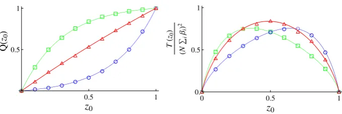
Fig. 2 Plots for the probability of fixation (left panel) and mean time to fixation (right panel) as a function of the projected initial conditions for theD= 3 island Moran model. The solid lines are calculated from the reduced model and the various symbols indicate the results obtained from simulations. For each different colour/symbol differentαvectors are used; green squares,α=(1,1,−1), red triangles,α=(−1,−1,1), and blue circles,α=(1,−2,−1). All other parameters are kept constant;s=0.005,N=200,β=(3,2,1) and the migration matrixmis fixed, though not given here. Simulation results are the average of 5000 runs
where
a1= D
i,j=1
u{1}i mi jfj
βi αj, b1=
D
i,j=1
u{1}i 2mi jfj
βi2 . (19)
Hereαi is the relative fitness of the first allele over the second on islandi andu{1}is the
left-eigenvector corresponding to the zero eigenvalue. So even with the added complexity of each island differing in size, arbitrary migration probabilities, selective advantage of allele 1 over allele 2 varying from island to island, and the number of islands itself arbitrary, the reduction gives a standard (i.e. non-spatial model) Moran model with selection with effective parameters which can be seen from Eq. (19) to contain information from virtually all the parameters of the original model. It should be noted that in order to prove results pertaining to the spectrum of the eigenvalues of the Jacobian, we assumed that the migration matrix had a structure which in effect meant that no subgroup of islands were isolated from any other [6], and so the results displayed in Eq. (19) are subject to this restriction. This rules out, for example, the case where the islands may be divided into two subgroups, with no migration between the subgroups.
As mentioned the reduced model is the mesoscopic version of the Moran (or, in fact, the Wright-Fisher model) with selection. The probability of either allele 1 or allele 2 fixing for a given initial state and also the mean time to fixation may be straightforwardly found [15], given as they are by the solution to second-order ordinary differential equations [7]. These are denoted byQ(z0)andT(z0)respectively. Herez0is the initial condition for the reduced
system, which was referred to asxCMICin the final paragraph of Sect.2.2on the first stage of
[image:14.439.50.390.51.165.2]master equation. Novel effects can be investigated through use of thes2term, and a greater range of parameters explored. We refer the reader to the original literature for a discussion of these [6,7].
3.1.2 TheD-Island Model with Mutation
So far in this article we have examined the effects of migration, selection and genetic drift, but not that other important process of population genetics: mutation. The inclusion of mutation has a drastic effect on the long term behaviour of the system, since it is now possible in principle for one allele to mutate to another at any time, and so concepts such as fixation probabilities and mean time to fixation do not apply. On the other hand, the pdf of the allele frequencies is now non-trivial and becomes stationary at long times. This is an interesting quantity which characterises the model and we use it to test the accuracy of the effective model found through the reduction procedure.
The microscopic model is constructed in a similar way to that described in Sect.2. There is more than one way that mutation can be included; here we follow the procedure described in Ref. [9]. In this case we allow birth/death/migration events to happen a fractionξof the time, and mutation events a fraction(1−ξ )of the time. The mutation rate from the first allele to the second on islandiis denoted byκi(1)and from the second to the first on islandiby
κi(2). It may be a little unusual to allow rates to vary from one island to the other, but allowing for this does not markedly increase the complexity of the calculation and so we include it.
If we denote the rates without mutation (such as are shown in Eq. (3) for the case of two islands) asTS(n′|n), where the subscript S indicates that selection has been included, but not
mutation, then the corresponding rates with mutation and selection included are
TMS(ni+1|ni)=ξTS(ni+1|ni)+(1−ξ ) κi(1)
(βiN −ni) βiN ,
TMS(ni−1|ni)=ξTS(ni−1|ni)+(1−ξ ) κi(2) ni βiN
. (20)
Here the dependence of the transition rates,TS(n′|n), on elements ofnthat do not change in
the transition has been suppressed. We may rescale time in the master equation by a factor ofξand absorb a factor of(1−ξ )/ξin the mutation rates. This effectively means that we can drop the factorsξand(1−ξ )from Eq. (20).
Making the diffusion approximation, the mesoscopic model is given by Eq. (7) with the noise correlator given by Eq. (8). In this case
Ai(x)|MS= Ai(x)|S+
1
βi
κi(1)−κi(1)+κi(2)xi, Bi j(x)
MS= Bi j(x)
S+O
κ(1),κ(2), (21)
whereκ(1)=(κ1(1), . . . , κD(1))andκ(2)=(κ1(2), . . . , κD(2)). Since mutation has been modelled as a linear process, theκ dependence inAi(x)in Eq. (21) is exact. We will neglect theκ
dependence inBi j(x)for precisely the same reasons that we neglected the dependence on
the selection coefficients: we are assuming that the elements ofκ(1)andκ(2)are so small that
they can be thought to be of the same order asN−1. We therefore only keep terms of order
κ(1)/N,κ(2)/N and 1/N2in the FPE.
(a) (b)
(c) (d)
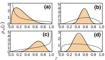
Fig. 3 The stationary pdf for theD-island Moran model on the slow subspace for a range of systems with various parameters which are omitted here for brevity but which can be found in Ref. [9]. The solid black line is obtained from an analysis of the reduced model, the orange histogram from simulations of the original microscopic model, and the dashed line from a well mixed model with the same total system size and average mutation rates (weighted by island size)
neutral model in exactly the same way as was done for selection strengths. Therefore the reduced model is given by Eqs. (7) and (8) withB(z)¯ unchanged from the form given in Eq. (18). Perhaps not surprisinglyA(z)¯ is modified by the addition of an extra term depending on the mutation rates [9]:
¯
AMS(z)= ¯AS(z)+ ˆκ(1)−
ˆ
κ(1)+ ˆκ(2)z=a1s z(1−z)+ ˆκ(1)−
ˆ
κ(1)+ ˆκ(2)z,
(22) where
ˆ
κ(1)= D
i=1 u{i1}κi(1)
βi
, κˆ(2)= D
i=1 u{i1}κi(2)
βi
. (23)
and wherea1is defined in Eq. (19). Here, as in Sect.3.1.1, we retain terms only to orders.
The stationary pdf of the effective theory can be straightforwardly found from the FPE corresponding to the SDE (7). Using the explicit forms forA(z)¯ andB(z)¯ one finds that [9]
pst(z)=Nzc1(1−z)c2exp(c3z), (24)
whereN is a normalisation constant and
c1= N b1ˆ
κ(1)−1, c2= N b1ˆ
κ(2)−1, c3=a1s N b1
. (25)
A comparison between simulations of the original model and calculations from the reduced model in Fig.3shows that the reduced model captures well the features of the full model.
[image:16.439.120.321.50.166.2]3.2 The Stochastic Lotka–Volterra Competition Model
The theory of evolution has had a very convoluted history, and a reflection of this was the significant contribution made to the subject by theoretical studies, at least compared to other areas of the biological sciences. This had repercussions on the nature of the mathematical models used in these studies: they tended to be unrelated to broader questions relating to the organism, and more focussed on the combinatorics of allele selection. This was a good strategy when trying to test the ideas of Darwinian evolution, but it tended to isolate the theoretical development of the subject from developments elsewhere.
An example is the Wright-Fisher model [22,65], one of the first models of genetic drift, as well as the precursor of the Moran model [44]. In this model there is no competition between individuals—a trait which is obviously a feature of Darwinian evolution. The population therefore grows very quickly, but is kept under control by sampling from the very large pool of individuals that come into existence, in order to form the next generation. Only a fixed number,N, of individuals are retained to form each new generation (Wright-Fisher) or births and deaths are coupled so the population at any given time is always equal toN (Moran). This leads to an artificiality in the way that the models are set-up.
In this section we will use as a starting point models in which the population is regulated by competition, rather than by a fictitious constraint which fixes the population size. This is a closer reflection of reality, and indeed the formulation of aspects of the models seem less contrived. It is a constant theme in the biological modelling literature that models of evolution should have a more ecological flavour, and this approach conforms to these views. An apparent disadvantage is that the number of variables is increased. To see that, recall that the Moran model of Sect.3.1had onlyDvariables, since the number of individuals carrying the second allele on islandicould be expressed in terms of the number of individuals carrying the first allele on the same islandi.e. N−ni. If the population of an island is not fixed, the number of individuals carrying the first and second allele can independently vary, and so the number of variables will double. Below we will describe how application of the reduction methods to models with competition show that they reduce to Moran-like models in the medium-to-long term [8,10]. The competition will be chosen to be of the simple Lotka–Volterra type [56], but in principle more complex competitive processes could be utilised. Since these are stochastic models, we will refer to them as stochastic Lotka–Volterra competition (SLVC) models.
3.2.1 TheD-Island SLVC Model
As indicated above this system has 2Dvariables which in the microscopic model aren(α)i , wherei =1, . . . ,Dlabels the islands andα =1,2 labels the allele. The comment made above concerning SLVC models being less contrived can be illustrated here in the way that migration is modelled. The procedure for doing this in the Moran model involves consider-able care in making sure that there are no biases built into the way the transition rates are constructed [see Eq. (3) in the simple two-island case] while keeping the population of both islands fixed. For example, one has to ensure that a death on islandjoccurs before a migra-tion from islandito this island is allowed. In the SLVC model, one simply specifies birth, death and competition rates, respectivelybi(α),di(α)andc(αβ)i , which are all independent of each other. For the neutral version of the model, the birth, death and competition rates are the same for all alleles (and are denoted by a superscript 0); selection is introduced through a small perturbation inǫ, whereǫis the selection strength:
b(α)i =bi(0)
1+ǫbˆ(α)i
, di(α)=di(0)
1+ǫdˆi(α)
, ci(αβ)=ci(0)
1+ǫcˆ(αβ)i
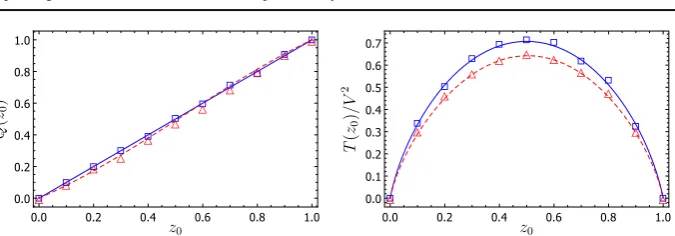
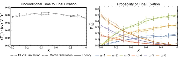
Fig. 4 Fixation probability of allele 1 (left panel) and mean unconditional time to fixation (right panel) as a function of the projected initial conditionz0for an SLVC model withD=4 islands in the neutral case (blue)
and in the case with selection (red,ǫ=0.05). Symbols: mean obtained from 3000 stochastic simulations of the microscopic system; lines: theoretical predictions for the fixation probability and mean time to fixation obtained from the reduced model. Here the parameterV is equal to 150 (Color figure online)
The diffusion approximation is applied in the same way as in the Moran model, although now the large parameter is notN, which is no longer present in the definition of the model, butV, which is some measure of the size of the system, such as the volume. Although there are 2Dvariables initially, 2D−1 of these are fast, and so the reduced model has again only one variable. It may be possible in some parameter regimes to see a clear cut decay first to theDvariables of a Moran-type model with fixed populations on each island, and then a slower decay to an effective one-island model, which parallels the discussion in Sect.3.1, but in many cases these time-scales will be similar or will overlap. The time-scales are related to the inverse of the eigenvalues of the Jacobian and, in general, these are complicated functions of all the model parameters.
While it is true that the reduced SLVCD-island model does reduce to a system which has a mesoscopic description given by Eqs. (11) and (14)—although withNreplaced byV—and withB(z)¯ =b1z(1−z)to leading order inǫ, the form ofA(z)¯ is a little different. It is found
to be given by [49]
¯
A(z)=ǫz(1−z) (a1−a2z)+Oǫ2. (27)
In this casea1,a2andb1are functions of the rates given which appear in Eq. (26),βi, and
the left-eigenvector of the Jacobian corresponding to the zero eigenvalue. This change in the form ofA(z)¯ may be slight, but it could give significantly different fixation probabilities and mean time to fixation. One reason for this is that it is now possible to have a fixed point in the deterministic dynamics. This dynamics will be given by Eq. (11) without the noise term, and so fixed points are solutions ofA(z)¯ =0. WhenA(z)¯ has the structure shown in Eq. (27), an internal fixed point (i.e.one not at the boundariesz=0 orz=1) is possible ifa2=0: z∗=a1/a2, where the asterisk denotes a fixed point. It will only exist if 0<a1/a2<1, but
if it is stable, it may prolong the time taken for the system to fix (reach the pointsz=0 or
z=1). Similarly if it is unstable, it may lead to a shorter mean time to fixation.
To test the approximation we again compare the fixation probabilities and mean fixation time derived from the reduced model and those found from simulations of the original model. Although the form ofA(z)¯ is slightly more complicated than before, it is nevertheless still straightforward to work with the ordinary differential equations forQ(z0)andT(z0). The
[image:18.439.54.392.41.159.2]3.2.2 The M-Allele SLVC Model
So far we have only discussed individuals which are haploid and carry one of two possible alleles. Here we discuss the generalisation toMalleles. This is interesting for a number of reasons, not least because we are able to recognise patterns that are not apparent in the two allele case. As in Sect.3.2.1, the variables in the microscopic model aren(α), where now
α=1, . . . ,Mand there is no island label, because we will assume that the population is well-mixed. In the corresponding haploid multiallelic Moran model there are onlyM−1 variables
n(a),a=1, . . . ,M−1, since the fixed population constraintM
α=1n(α)=N, means that n(M)can be expressed in terms of the otherM−1 variables:n(M)=N−aM=−11 n(a). Here
the Greek indicesα, β, . . .will always run from 1 toMand the Roman indicesa,b, . . .will always run from 1 toM−1.
Previously we used the reduction method to obtain an effective model which was amenable to analysis. Here will have a different perspective: we will ask if we can perform a reduction on the multiallelic SLVC model with M variables to the multiallelic Moran model with
M−1 variables. If this is so, then the more natural SLVC model will give the same results as the Moran model at medium and long times. From a mathematical point of view, the difference between the reduction described in Sect.3.1and in Sect.3.2.1is that previously there wereD−1 or 2D−1 fast modes, and a single slow mode, whereas here there is one fast mode andM−1 slow modes, thus giving an effective model which is(M−1)dimensional [10].
The reduction procedure has been carried out in Ref. [10]. An equation analogous to Eq. (11) is found, but now in(M−1)variables:
dz(a)
dτ = A
(a)(z)+√1 V ζ
(a)(τ ), a=1, . . . ,M−1, (28)
whereζ(a)(τ )is a Gaussian noise with zero mean and with a correlator
ζ(a)(τ )ζ(b)(τ′)= 2b
(0)c(0)
b(0)−d(0)2
z(a)δab−z(a)z(b)
δτ−τ′. (29)
Here, the notation of underlining a vector is used for(M−1)-dimensional vectors and bold forM-dimensional vectors. The correlation function is given to zeroth order inǫ, which is the neutral model result. It is exactly the form found in theM-allele Moran model, up to some rescalings which are absorbed into the new timeτ[10]. In the neutral caseA=0, and the SLVC model reduces exactly to the Moran model at medium to long times, after rescaling the time.
If selection is included,Ais no longer equal to zero. In order to aid the comparison with the Moran model, it is useful to introduce two quantities:
ˆ
C(ab)≡ ˆc(ab)− ˆc(a M)− ˆc(Mb)+ ˆc(M M), (30) and
(α)≡ b
(0)bˆ(α)−d(0)dˆ(α)
ThenAa(z)takes the form
A(a)(z)=ǫz(a) ⎧ ⎨
⎩
(a)− ˆc(a M)−(M)− ˆc(M M)
−
M−1
b=1
(b)− ˆc(bM)−(M)− ˆc(M M)z(b)
−
M−1
b=1 ˆ
C(ab)z(b)+ M−1
b,c=1 ˆ
C(bc)z(b)z(c) ⎫ ⎬
⎭+
O(ǫ2). (32)
For now, we note that, just as in Eq. (27),Ais cubic in the components ofz. This is an important point in mappings between reduced SLVC and Moran models, as we will now see. We begin our discussion with theM-allele Moran model in the case where the selection is frequency independent, that is, when the weight functionsW(α), analogous to those intro-duced in Eq. (3), are independent ofn. Specifically we assume thatW(α)=1+ρ(α)s, where theρ(α)are constants. This is the case that we have examined so far in this paper. Then we find, after making the diffusion approximation, a model given by Eqs. (28), (29) and (32), but only ifCˆ(ab)=0 for allaandb[10]. If this condition holds, the reduced SLVC model and the Moran model with frequrncy independent selection match, provided that we make the identificationρ(α)=(α)− ˆc(αM). We also need to match up the selection strength used in the SLVC model (ǫ) to the one used in the Moran model (s). The relation between them is:
s=ǫ(b(0)−d(0))/b(0). Although some care has to be taken with making the identification
between the two models [10], one can note that the function Ain the Moran model with frequency dependent selection is quadratic, and Eq. (32) is cubic in general, so the condition
ˆ
C(ab)=0 gives the possibility of a direct mapping between the two models.
We have assumed that selection is frequency independent so far, since this is the usual supposition made by many population geneticists and historically was the standard assump-tion used. However this may simply be a theoretical prejudice, since if one wishes to allow the fitness weightingsW(α) to depend on the composition of the population, one has to devise a model for this dependence, and so frequency independence is the simplest and most convenient choice. In addition, there are hints from experimental investigations that even if there are attempts to suppress factors that might lead to frequency dependent selection, it still seems to emerge [41]. Therefore it seems important to devise a natural way of including frequency dependence in modelling selection. Fortunately, there does exist a methodology to do this. It is based on ideas from game theory, where each allele “plays” a game with every other allele in the population [47]. In the way we choose to implement this [10], the fitness weightings are taken to have the form
W(α)(n)=1+s M−1
b=1 g(αb)n
(b) N +g
(αM)
1−
M−1
b=1 n(b)
N
, (33)
whereg(αβ)is the payoff to alleleαfrom interacting with typeβ.
We can now make the diffusion approximation, just as in the frequency independent case, but now usingW(α)(n)given by Eq. (33), rather than then-independent formW(α)=
1+ρ(α)s. Clearly, the structure ofW(α)(n)in Eq. (33) can potentially lead to more complicated
sz(a) ⎡
⎣G(a M)+ M−1
b=1
G(ab)z(b)−
M−1
b=1
G(bM)z(b)−
M−1
b,c=1
G(bc)z(b)z(c) ⎤
⎦, (34) which is of exactly the same form as that given by Eq. (32). To get the precise correspondence between the two models one must takeG(ab)= − ˆC(ab)for allaandb, whereG(ab)has the same structure as is displayed forCˆ(ab)in Eq. (30), namely
G(aβ)≡g(aβ)−g(Mβ); G(ab)≡G(ab)−G(a M). (35) In addition the identificationg(αM)=(α)− ˆc(αM)has to be made [10]. The fact that it is onlyG(a M)andG(ab), and notg(αβ)alone, that appear in the expression forAis interesting,
since the quantityG(aβ)can be interpreted as a relative fitness, namely the payoff to allelea
against an opponentβrelative to the payoff to alleleMagainst the same opponent. Similarly,
G(ab)is a relative relative fitness. Therefore, as one would expect, it is not the actual payoffs which are important, but their values relative to the other payoffs.
In Sect.3.2.1we discussed how existence of an interior fixed point, that is, one not on the boundaries, could lead to different fixation probabilities and mean times to fixation. To investigate the possible existence of such fixed points in the frequency dependentM-allele case, we setA(a)(z), given by Eq. (34), to zero. Now summing this expression overagives
0=
1−
M−1
a=1 z(a)
⎧ ⎨
⎩ M−1
b=1
G(bM)z(b)+
M−1
b,c=1
G(bc)z(b)z(c) ⎫ ⎬
⎭
. (36)
If the fixed point is not to be on the boundary, thenaM=−11 z(a) =1 and so the second bracket in Eq. (36) must vanish. Substituting this condition into the expression (34), which is itself taken to be zero, gives the fixed point equation to beG(a M)+M−1
b=1 G(ab)z(b)=0, since z(a)=0 for internal fixed points. Since this non-boundary fixed point equation is linear, there can generically be at most one fixed point. The position of this fixed point can therefore easily be found, and a determination made as to whether it lies in the SS and is therefore admissible. A similar analysis for the frequency independent case yields the conditionρ(a) =ρ(M)for alla. However, if all theρ(α)are equal there is no selection, so in the case of frequency
independent selection there are no interior fixed points.
The finding that the more realistic SLVC model reduces to the Moran model with frequency dependent selection is another reason to use frequency dependence in the modelling of selection in the Moran model. Although, as we have already remarked, the resulting Moran model is still(M−1)-dimensional, and so difficult to analyse, some progress can still be made in some cases [10]. In this way the SLVC model may, in effect, be analysed. An example of such a situation is shown in Fig.5.
3.3 Diploid Moran Model with Sexual Reproduction: The Hardy–Weinberg Assumption from First Principles
In the Moran model discussed in Sects.2and3.1, individuals are haploid (they carry only a single allele) and reproduction occurs asexually (individuals simply duplicate themselves). While this is a relevant case for certain simple organisms, it is less so for many complex organisms which are diploid and reproduce sexually, such as animals.
Fig. 5 Plots of the unconditional mean time until the fixation of a single allele/species and the probability of the fixation of an allele/species for the Moran and SLVC models with frequency-independent selection in the caseM=6 alleles/species. In these plots all alleles in the Moran model are under one of two selection pressures, while in the SLVC model all species have differing parameters that combine to give two selection pressures, making the system mappable to the Moran model presented. Analytical results are only available for the probability of fixation. Simulations results are the mean of 103stochastic simulations of the Moran and SLVC models. Parameters used are given Ref. [10], where the parameterization ofx(0)in terms ofκis also described
possible genotypes in the population; here we will denote the homozygotes by A(1)A(1)and A(2)A(2), while the heterozygotes will be denoted by A(1)A(2). If we fix the population size to beN, this leaves two free variables. As we have previously discussed, this makes obtaining analytic quantities in the model far more difficult than in the asexual haploid case, where the system was described by a single variable.
Classic ApproachClassic studies in population genetics circumvented this complexity by building single variable models that implicitly exploited a separation of timescales. It was noticed early on in theoretical population genetics that if there were no fitness differences between the genotypes (i.e. the system was neutral) the frequency of genotypes in such a diploid system would quickly relax to Hardy–Weinberg frequencies [31,63], where the number of each genotype could be described in terms of a single variable, the frequency of one of the alleles. In the terminology of our present paper, the system would quickly relax to a CM. Denoting the allele frequencies byx(1) =n(A(1))/(2N)andx(2)=n(A(2))/2N =
(1−x(1)), and the genotype frequencies by y(1) = n(A(1)A(1))/N, y(2) = n(A(1)A(2))/N,
y(3)=n(A(2)A(2))/N =(1−y(1)−y(2)), this is given by [20]
y(1)=x(1)2, y(2)=2x(1)1−x(1), y(3)=1−x(1)2 . (37) Rather than model the dynamics of the diploid population, the dynamics of thealleles
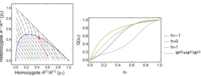
were modelled with the assumption that they existed at Hardy–Weinberg frequencies. This was assumed to also hold when selection was sufficiently weak that the deviations from these “equilibrium” frequencies were not too great [44] (note the conceptual similarities with our approach). Genotypes AA are assumed to be under selective pressure A(1)A(1), genotypes A(1)A(2)under(1+sh)and genotypes A(2)A(2)under 1 [20]. Note then that choosingh>1 corresponds to overdominance, whileh≤1 corresponds to underdominance [20]. The details are given in Appendix A, however upon applying the diffusion approximation one obtains an FPE (6) or SDE (7), with [20]
Ax(1)=sx(1)1−x(1) x(1)+h1−2x(1), B
x(1)
=2x(1)
1−x(1)
[image:22.439.51.394.51.159.2]