This is a repository copy of On the Runtime Analysis of the Clearing Diversity-Preserving
Mechanism.
White Rose Research Online URL for this paper:
http://eprints.whiterose.ac.uk/130670/
Version: Accepted Version
Article:
Covantes Osuna, E. and Sudholt, D. orcid.org/0000-0001-6020-1646 (2018) On the
Runtime Analysis of the Clearing Diversity-Preserving Mechanism. Evolutionary
Computation. ISSN 1063-6560
https://doi.org/10.1162/evco_a_00225
[email protected] https://eprints.whiterose.ac.uk/ Reuse
Items deposited in White Rose Research Online are protected by copyright, with all rights reserved unless indicated otherwise. They may be downloaded and/or printed for private study, or other acts as permitted by national copyright laws. The publisher or other rights holders may allow further reproduction and re-use of the full text version. This is indicated by the licence information on the White Rose Research Online record for the item.
Takedown
If you consider content in White Rose Research Online to be in breach of UK law, please notify us by
On the Runtime Analysis of the Clearing
Diversity-Preserving Mechanism
Edgar Covantes Osuna and Dirk Sudholt
Department of Computer Science University of Sheffield, United Kingdom
May 10, 2018
Abstract
Clearing is a niching method inspired by the principle of assigning the available resources among a niche to a single individual. The clearing procedure supplies these resources only to the best individual of each niche: the winner. So far, its analysis has been focused on experi-mental approaches that have shown that clearing is a powerful diversity-preserving mechanism. Using rigorous runtime analysis to explain how and why it is a powerful method, we prove that a mutation-based evolutionary algorithm with a large enough population size, and a pheno-typic distance function always succeeds in optimising all functions of unitation for small niches in polynomial time, while a genotypic distance function requires exponential time. Finally, we prove that with phenotypic and genotypic distances clearing is able to find both optima for
Twomaxand several general classes of bimodal functions in polynomial expected time. We
use empirical analysis to highlight some of the characteristics that makes it a useful mechanism and to support the theoretical results.
1
Introduction
Evolutionary Algorithms (EAs) with elitist selection are suitable to locate the optimum of unimodal functions as they converge to a single solution of the search space. This behaviour is also one of the major difficulties in a population-based EA, the premature convergence toward a suboptimal individual before the fitness landscape is explored properly. Real optimisation problems, however, often lead to multimodal domains and so require the identification of multiple optima, either local or global (Sareni and Krahenbuhl,1998;Singh and Deb,2006).
In multimodal optimisation problems, there exist many attractors for which finding a global op-timum can become a challenge to any optimisation algorithm. A diverse population can deal with multimodal functions and can explore several hills in the fitness landscape simultaneously, so they can therefore support global exploration and help to locate several local and global optima. The algorithm can offer several good solutions to the user, a feature desirable in multiobjective optimi-sation. Also, it provides higher chances to find dissimilar individuals and to create good offspring with the possibility of enhancing the performance of other procedures such as crossover (Friedrich et al.,2009).
Diversity-preserving mechanisms provide the ability to visit many and/or different unexplored regions of the search space and generate solutions that differ in various significant ways from those seen before (Gendreau and Potvin,2010;Lozano and Garc´ıa-Mart´ınez, 2010). Most analyses and comparisons made between diversity-preserving mechanisms are assessed by means of empirical investigations (Chaiyaratana et al., 2007; Ursem, 2002) or theoretical runtime analyses (Jansen and Wegener, 2005; Friedrich et al., 2007; Oliveto and Sudholt, 2014; Oliveto et al., 2014; Gao and Neumann,2014;Doerr et al.,2016). Both approaches are important to understand how these mechanisms impact the EA runtime and if they enhance the search for obtaining good individuals. These different results imply where/which diversity-preserving mechanism should be used and, perhaps even more importantly, where they should not be used.
outside their group. Species can be defined as similar individuals of a specific niche in terms of similarity metrics. In EAs the term niche is used for the search space domain, and species for the set of individuals with similar characteristics. By analogy, niching methods tend to achieve a natural emergence of niches and species in the search space (Sareni and Krahenbuhl,1998).
A niching method must be able to form and maintain multiple, diverse, final solutions for an exponential to infinite time period with respect to population size, whether these solutions are of identical fitness or of varying fitness. Such requirement is due to the necessity to distinguish cases where the solutions found represent a new niche or a niche localised earlier (Mahfoud, 1995).
Niching methods have been developed to reduce the effect of genetic drift resulting from the selection operator in standard EAs. They maintain population diversity and permit the EA to investigate many peaks in parallel. On the other hand, they prevent the EA from being trapped in local optima of the search space (Sareni and Krahenbuhl,1998). In the majority of algorithms, this effect is attained due to the modification of the process of selection of individuals, which takes into account not only the value of the fitness function but also the distribution of individuals in the space of genotypes or phenotypes (Glibovets and Gulayeva,2013).
Many researchers have suggested methodologies for introducing niche-preserving techniques so that, for each optimum solution, a niche gets formed in the population of an EA. Most of the analyses and comparisons made between niching mechanisms are assessed by means of empirical investigations using benchmark functions (Sareni and Krahenbuhl, 1998; Singh and Deb, 2006). There are examples where empirical investigations are used to support theoretical runtime analyses and close the gap between theory and practice (Friedrich et al.,2009;Oliveto et al.,2014;Oliveto and Zarges,2015;Covantes Osuna and Sudholt,2017;Covantes Osuna et al.,2017).
Both fields use artificially designed functions to highlight characteristics of the studied EAs when tackling optimisation problems. They exhibit such properties in a very precise, distinct, and paradigmatic way. Moreover, they can help to develop new ideas for the design of new variants of EAs and other search heuristics. This leads to valuable insights about new algorithms on a solid basis (Jansen,2013).
Most of the theoretical analyses are made on example functions with a clear and concrete structure so that they are easy to understand. They are defined in a formal way and allow for the derivation of theorems and proofs allowing to develop knowledge about EAs in a sound scientific way. In the case of empirical analyses, most of the results are based on the analysis of more complex example functions and algorithmic frameworks for a specific set of experiments. This approach allows to explore the general characteristics more easily than in the theoretical field.
Our contribution is to provide a rigorous theoretical runtime analysis for theclearingdiversity mechanism, to find out whether the mechanism is able to provide good solutions by means of experiments, and we include theoretical runtime analysis to prove how and why an EA is able to obtain good solutions depending on how the population size,clearing radius, niche capacity, and the dissimilarity measure are chosen.
This manuscript extends a preliminary conference paper (Covantes Osuna and Sudholt, 2017) in the following ways. We extend the theory for large niches by looking into the choice of the pop-ulation size. While it was known that a poppop-ulation size ofµ≥κn2/4 is sufficient (Covantes Osuna
and Sudholt, 2017), here we show that population sizes of at least Ω(n/polylog(n)) are necessary to escape from local optima. The reason is that for smaller population sizes, winners in local optima spawn offspring that repeatedly take over the whole population, and this happens before individuals can escape from the optima’s basin of attraction. We further extend our analysis to more general classes of examples landscapes defined by Jansen and Zarges(2016), showing that clearingis effective across a range of functions with different slopes and optima having different basins of attraction. Finally, we extend the experimental analysis for smaller population sizes ofµ
with smalln= 30 and largen= 100.
In the remainder of this paper, we first present the algorithmic framework in Section2. The definition of clearing, algorithmic approach, and dissimilarity measures are defined in Section 3. The theoretical analysis is divided in Sections4 and5 for small and large niches, respectively. In Section4 we show how clearingis able to solve, for small niches and the right distance function, all functions of unitation, and in Section 5 we show how the population dynamics with large population size in clearing solves Twomax with the most natural distance function: Hamming
general behaviour of the algorithm and providing a closer look into the impact of the population size on performance. We present our conclusions in Section 8, giving additional insight into the dynamic behaviour of the algorithm.
2
Preliminaries
We focus our analysis on the simplest EA with a finite population called (µ+1) EA (hereinafter,
µ denotes the size of the current population, see Algorithm 1). Our aim is to develop rigorous runtime bounds of the (µ+1) EA with the clearingdiversity mechanism. We want to study how diversity helps to escape from some optima. The (µ+1) EA uses random parent selection and elitist selection for survival and has already been investigated byWitt(2006).
Algorithm 1(µ+1) EA
1: Lett:= 0 and initialise P0 withµindividuals chosen uniformly at random.
2: whileoptimumnotfounddo
3: Choosex∈Pt uniformly at random.
4: Createy by flipping each bit inxindependently with probability 1/n. 5: Choosez∈Pt with worst fitness uniformly at random.
6: if f(y)≥f(z)thenPt+1=Pt\ {z} ∪ {y}else Pt+1=Pt end if
7: Lett:=t+ 1. 8: end while
We consider functions of unitationf :{0,1}n→R, wheref(x) depends only on the number of
1-bits contained in a stringxand is always non-negative, i. e., f is entirely defined by a function
u : {0, . . . , n} → R+, f(x) = u(|x|
1), where |x|1 denotes the number of 1-bits in individual x.
In particular, we consider the bimodal function of unitation calledTwomax (see Definition2.1)
for the analysis of large niches. Twomaxcan be seen as a bimodal equivalent of Onemax. The
fitness landscape consists of two hills with symmetric slopes. In contrast toFriedrich et al.(2009) where an additional fitness value for 1n was added to distinguish between a local optimum 0n
and a unique global optimum, we have opted to use the same approach asOliveto et al. (2014), and leave unchangedTwomax since we aim at analysing the global exploration capabilities of a
population-based EA.
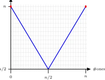
Definition 2.1(Twomax). A bimodal function of unitation which consists of two different sym-metric slopes Zeromaxand Onemaxwith0n and1n as global optima, respectively.
Twomax(x) := max
( n
X
i=1
xi, n− n
X
i=1
xi
)
.
The fitness of ones increases with more than n/2 1-bits, and the fitness of zeroes increases with less than n/2 1-bits. These sets are refereed as branches. The aim is to find a population containing both optima (see Figure1).
#ones
n/2 0
n
[image:4.595.211.386.620.753.2]n/2 n
We analyse the expected time until both optima have been reached. Twomax is an ideal
benchmark function forclearingas it is simply structured, hence facilitating a theoretical analysis, and it is hard for EAs to find both optima as they have the maximum possible Hamming distance. Its choice further allows comparisons with previous approaches like inFriedrich et al.(2009) and
Oliveto et al.(2014) in the context of diversity-preserving mechanisms.
The (µ+1) EA with no diversity-preserving mechanism (Algorithm1) has already been analysed for theTwomaxfunction. The selection pressure is quite low, nevertheless, the (µ+1) EA is not
able to maintain individuals on both branches for a long time. Without any diversification, the whole population of the (µ+1) EA collapses into the 0n branch with probability at least 1/2−o(1)
(seeMotwani and Raghavan,1995for the asymptotic notation) in timenn−1, once the population
contains copies of optimum individuals in one of the two branches, it will be necessary to flip all the bits at the same time in order to allow that individual to survive and find both optima on
Twomax, so the expected optimisation time is Ω(nn) (Friedrich et al.,2009, Theorem 1).
Adding other diversity-preserving mechanisms into the (µ+1) EA like avoiding genotype or phenotype duplicates does not work, the algorithm cannot maintain individuals in both branches, so the population collapse into the 0nbranch with probability at least 1/2−o(1) with an expected
optimisation time of Ω(nn−1) and 2Ω(n) (Friedrich et al., 2009, Theorem 2 and 3), respectively.
Deterministic crowding with sufficiently large population is able to reach both optima with high probability in expected timeO(µnlogn) (Friedrich et al.,2009, Theorem 4).
Amodified version of fitness sharing is analysed inFriedrich et al.(2009): rather than selecting individuals based on their shared fitness, selection was done on a level of populations. The goal was to select the new population out of the union of all parents and all offspring such that it maximises the overall shared fitness of the population. The drawback of this approach is that all possible size-µsubsets of this union of sizeµ+λ, whereλis the number of offspring, need to be examined. For largeµandλ, this is prohibitive. It is proved that a population-based shared fitness approach withµ≥2 reaches both optima of Twomaxin expected timeO(µnlogn) (Friedrich et al.,2009,
Theorem 5).
InOliveto et al.(2014), the performance of the originalfitness sharing approach is analysed. The analysis showed that using the conventional (phenotypic) sharing approach leads to consider-ably different behaviours. A population sizeµ= 2 is not sufficient to find both optima onTwomax
in polynomial time: with probability 1/2 + Ω(1) the population will reach the same optimum, and from there the expected time to find both optima is Ω(nn/2) (Oliveto et al., 2014, Theorem 1).
However, there is still a constant probability Ω(1) to find both optima in polynomial expected time
O(nlogn), if the two search points are initialised on different branches, and if these two search points maintain similar fitness values throughout the run (Oliveto et al.,2014, Theorem 2).
Withµ≥3, once the population is close enough to one optimum, individuals descending the branch heading towards the other optimum are accepted. This threshold, that allows successful runs with probability 1, lies further away from the local optimum as the population size increases finding both optima in expected timeO(µnlogn) (Oliveto et al.,2014, Theorem 3). Concerning the effects of the offspring population, increasing the offspring population of a (µ+λ) EA, with
µ= 2 andλ≥µcannot guarantee convergence to populations with both optima, i. e., depending onλone or both optima can get lost, the expected time for finding both optima is Ω(nn/2) (Oliveto et al.,2014, Theorem 4).
3
Clearing
Clearing is a niching method inspired by the principle of sharing limited resources within a niche (or subpopulation) of individuals characterised by some similarities. Instead of evenly sharing the available resources among the individuals of a niche, theclearingprocedure supplies these resources only to the best individual of each niche: the winner. The winner takes all rather than sharing resources with the other individuals of the same niche as it is done with fitness sharing (P´etrowski,
1996).
to zero1. With such a mechanism, two approaches can be considered. For a given population,
the set of winners is unique. The winner and all the individuals that it dominates are then fictitiously removed from the population. Then the algorithm proceeds in the same way with the new population which is then obtained. Thus, the list of all the winners is produced after a certain number of steps.
On the other hand, the population can be dominated by several winners. It is also possible to generalise theclearingalgorithm by accepting several winners chosen among theniche capacity
κ (best individuals of each niche defined as the maximum number of winners that a niche can accept). Thus, choosing niching capacities between one and the population size offers intermediate situations between the maximumclearing(κ= 1) and a standard EA (κ≥µ).
Empirical investigations made in P´etrowski (1996, 1997a,b); Sareni and Krahenbuhl (1998);
Singh and Deb (2006) mentioned that clearing surpasses all other niching methods because of its ability to produce a great quantity of new individuals by randomly recombining elements of different niches, controlling this production by resetting the fitness of the poor individuals in each different niche. Furthermore, an elitist strategy prevents the rejection of the best individuals.
We incorporate theclearingmethod into Algorithm1, resulting in Algorithm2. The idea behind Algorithm2 is: once a population withµindividuals is generated, an individualxis selected and changed according to mutation. A temporary populationP∗
t is created from populationPtand the
offspringy, then the fitness of each individual inP∗
t is updated according to theclearingprocedure
shown in Algorithm3.
Algorithm 2(µ+1) EA with clearing
1: Lett:= 0 and initialise P0 withµindividuals chosen uniformly at random.
2: whileoptimumnotfounddo
3: Choosex∈Pt uniformly at random.
4: Createy by flipping each bit inxindependently with probability 1/n. 5: LetP∗
t =Pt∪ {y}.
6: Updatef(P∗
t) with the clearing procedure (Algorithm 3).
7: Choosez∈Pt with worst fitness uniformly at random.
8: if f(y)≥f(z)thenPt+1=Pt∗\ {z} elsePt+1=Pt∗\ {y}end if
9: Lett:=t+ 1. 10: end while
Each individual is compared with the winner(s) of each niche in order to check if it belongs to a certain niche or not, and to check if its a winner or if it is cleared. Here d(P[i], P[j]) is any dissimilarity measure (distance function) between two individualsP[i] andP[j] of population P. Finally, we keep control of theniche capacitydefined byκ. For the sake of clarity, the replacement policy will be the one defined inWitt(2006): the individuals with best fitness are selected (set of winners) and individuals coming from the new generation are preferred if their fitness values are at least as good as the current ones (novelty is rewarded).
Algorithm 3Clearing
1: SortP according to fitness of individuals by decreasing values. 2: fori:= 1 to|P|do
3: if f(P[i])>0 then
4: winners:= 1
5: forj:=i+ 1 to|P|do
6: if f(P[j])>0and d(P[i], P[j])< σthen
7: if winners < κthenwinners:=winners+ 1else f(P[j]) := 0end if
8: end if
9: end for
10: end if
11: end for
Finally, as dissimilarity measures, we have considered genotypic or Hamming distance, defined
as the number of bits that have different values inxandy: d(x, y) := H(x, y) := Pin=0−1|xi−yi|,
and phenotypic (usually defined as Euclidean distance between two phenotypes). AsTwomaxis
a function of unitation, we have adopted the same approach as in previous work (Friedrich et al.,
2009; Oliveto et al., 2014) for the phenotypic distance function, allowing the distance function d to depend on the number of ones: d(x, y) := | |x|1− |y|1| where|x|1 and |y|1 denote the number
of 1-bits in individualxandy, respectively.
4
Small Niches
In this section we prove that the (µ+1) EA with phenotypic clearing and a small niche capacity is not only able to achieve both optima of Twomaxbut is also able to optimise all functions of
unitation with a large enough population, while genotypic clearing fails in achieving such a task (hereinafter, we will refer as phenotypic or genotypic clearing to Algorithm3 with phenotypic or genotypic distance function, respectively).
4.1
Phenotypic Clearing
First it is necessary to define a very important property of clearing, which is its capacity of preventing the rejection of the best individuals in the (µ+1) EA, and once µ is defined large enough,clearingand the population size pressure will always optimise any function of unitation.
Note that on functions of unitation all search points with the same number of ones have the same fitness, and for phenotypic clearing with clearing radius σ = 1 all search points with the same number of ones form a niche. We refer to the set of all search points withiones as nichei. In order to find an optimum for any function of unitation, it is sufficient to have all nichesi, for 0≤i≤n, being present in the population.
In the (µ+1) EA with phenotypic clearing withσ = 1, κ∈N and µ≥(n+ 1)·κ, a niche i
can only containκwinners with i ones. The condition onµensures that the population is large enough to store individuals from all possible niches.
Lemma 4.1. Consider the(µ+1) EAwith phenotypic clearing withσ= 1,κ∈Nandµ≥(n+1)·κ
on any function of unitation. Then winners are never removed from the population, i. e., ifx∈Pt
is a winner thenx∈Pt+1.
Proof. After the first evaluation with clearing, individuals dominated by other individuals are cleared and the dominant individuals are declared as winners. Cleared individuals are removed from the population when new winners are created and occupy new niches. Once an individual becomes a winner, it can only be removed if the size of the population is not large enough to maintain it, as the worst winner is removed if a new winner reaches a new better niche. Since there are at mostn+ 1 niches, each having at mostκwinners, ifµ≥(n+ 1)·κthen there must be a cleared individual amongst theµ+ 1 parents and offspring considered for deletion at the end of the generation. Thus, a cleared individual will be deleted, so winners cannot be removed from the population.
The behaviour described above means, that with the defined parameters and sufficiently largeµ
to occupy all the niches, we have enough conditions for the furthest individuals (individuals with the minimum and maximum number of ones in the population) to reach the opposite edges. Now that we know that a winner cannot be removed from the population by Lemma4.1, it is just a matter of finding the expected time until 0n and 1n are found.
Because of the elitist approach of the (µ+1) EA, winners will never be replaced if we assume a large enough population size. In particular, the minimum (maximum) number of ones of any search point in the population will never increase (decrease). We first estimate the expected time until the two most extreme search points 0n and 1n are being found, using arguments similar to
the well-known fitness-level method (Wegener,2002).
Lemma 4.2. Let f be a function of unitation and σ= 1, κ∈N andµ≥(n+ 1)·κ. Then, the
expected time for finding the search points0n and1n with the (µ+1) EAwith phenotypic clearing
onf isO(µnlogn).
Proof. First, we will focus on estimating the time until the 1n individual is found (by symmetry,
search point isi, it has a probability of being selected at least of 1/µ. In order to create a niche withj > iones, it is just necessary that one of then−i zeroes is flipped into 1-bit and the other bits remains unchanged. Each bit flip has a probability of being changed (mutated) of 1/n and the probability of the other bits remaining unchanged is (1−1/n)n−1. Hence, the probability of
creating some niche withj > iones is at least
1
µ· n−i
n ·
1−n1
n−1
≥nµen−i.
The expected time for increasing the maximum number of ones,i, is hence at most (µen)/(n−i) and the expected time for finding 1n is at most
n−1
X
i=0
µen
n−i =µen
n
X
i=1
1
i ≤µenlnn=O(µnlogn).
Where the summation Hn =Pni=11/i is known as the harmonic number and satisfies Hn =
lnn+ Θ(1). Adding the same time for finding 0n proves the claim.
Once the search points 0n and 1n have been found, we can focus on the time required for the algorithm until all intermediate niches are discovered.
Lemma 4.3. Let f be any function of unitation, σ= 1,κ∈N andµ≥(n+ 1)·κ, and assume
that the search points0n and1n are contained in the population. Then, the expected time until all
niches are found with the(µ+1) EAwith phenotypic clearing on f isO(µn).
Proof. According to Lemma 4.1 and the elitist approach of (µ+1) EA, winners will never be replaced if we assume a large enough population size and by assumption we already have found both search points 0n and 1n.
As long as the algorithm has not yet found all niches with at leastn/2 ones, then there must be an index i≥ n/2 such that the population does not cover the niche with i ones, but it does cover the niche withi+ 1 ones. We can mutate an individual from nichei+ 1 to populate niche
i. The probability of selecting an individual from niche i+ 1 is at least 1/µ, and since it is just necessary to flip one of at leastn/2 0-bits with probability 1/n, we have a probability of at least 1/2 to do so, and a probability of leaving the remaining bits untouched of (1−1/n)n−1 ≥1/e.
Together, the probability is bounded from below by 1/(2µe). Using the level-based argument used before for the case of the niches, the expected time to occupy all niches with at leastn/2 ones is bounded by
n−1
X
i=n/2
2µe
1 ≤2µen=O(µn).
A symmetric argument applies for the niches with fewer thann/2 ones, leading to an additional time ofO(µn).
Theorem 4.4. Let f be a function of unitation and σ= 1,κ∈Nand µ≥(n+ 1)·κ. Then, the
expected optimisation time of the(µ+1) EAwith phenotype clearing on f isO(µnlogn).
Proof. Now that we have defined and proved all conditions where the algorithm is able to maintain every winner in the population (Lemma4.1), to find the extreme search points (Lemma4.2) and intermediate niches (Lemma4.3) of the function f, we can conclude that the total time required to optimise the function of unitationf isO(µnlogn).
4.2
Genotypic Clearing
In the case of genotypic clearing withσ= 1, the (µ+1) EA behaves like the diversity-preserving mechanism calledno genotype duplicates. The (µ+1) EA with no genotype duplicates rejects the new offspring if the genotype is already contained in the population. The same happens for the (µ+1) EA with genotypic clearing andσ= 1 if the population is initialised withµmutually different genotypes (which happens with probability at least 1− µ2
2−n). In other words, conditional on the
population being initialised with mutually different search points, both algorithms are identical. In
andµ=o(n1/2) is not powerful enough to explore the landscape and can be easily trapped in one
optimum of Twomax. Adapting Friedrich et al. (2009, Theorem 2) to the goal of finding both
optima and noting that µ22−n=o(1) for the consideredµyields the following.
Corollary 4.5. The probability that the(µ+1) EAwith genotypic clearing,σ= 1andµ=o(n1/2)
finds both optima on Twomax in timenn−2 is at most o(1). The expected time for finding both
optima isΩ(nn−1).
As mentioned before, the use of a proper distance is really important in the context ofclearing. In our case, we use phenotypic distance for functions of unitation, which has been proved to provide more significant information at the time it is required to define small differences (in our case small niches) among individuals in a population, so the use of that knowledge can be taken into consideration at the time the algorithm is set up. Otherwise, if there is no more knowledge related to the specifics of the problem, genotypic clearing can be used but with larger niches as shown in the following section.
5
Large Niches
While small niches work with phenotypic clearing, Corollary4.5showed that with genotypic clear-ing small niches are ineffective. This makes sense as for phenotypic clearclear-ing with σ= 1 a niche withiones covers nisearch points, whereas a niche in genotypic clearing with σ= 1 only covers one search point. In this section we turn our attention to larger niches, where we will prove that cleared search points are likely to spread, move, and climb down a branch.
We first present general insights into these population dynamics withclearing. These results capture the behaviour of the population in the presence of only one winning genotypex∗(of which there may beκcopies). We estimate the time until in this situation the population evolves a search point of Hamming distance dfrom said winner, for any d ≤σ, or for another winner to emerge (for example, in case an individual of better fitness thanx∗is found).
These time bounds are very general as they are independent of the fitness function. This is possible since, assuming the winners are fixed atx∗, all other search points within the clearing radiusreceive a fitness of 0 and hence are subject to a random walk. We demonstrate the usefulness of our general method by an application toTwomaxwith aclearing radius ofσ=n/2, where all
winners are copies of either 0n or 1n. The results hold both for genotypic clearing and phenotypic
clearing as the phenotypic distance of any pointxto 0n (1n, resp.) equals the Hamming distance
ofxto 0n (1n, resp.).
5.1
Large Population Dynamics with Clearing
We assume that the population contains only one winner genotypex∗, of which there areκcopies. For any given integer 0≤d≤σ, we analyse the time for the population to reach a search point of Hamming distance at leastdfromx∗, or for a winner different fromx∗ to emerge. To this end, we will study a potential functionϕthat measures the dynamics of the population. Let
ϕ(Pt) =
X
x∈Pt
H(x, x∗)
be the sum of all Hamming distances of individuals in the population to the winner x∗. The following lemma shows how the potential develops in expectation.
Lemma 5.1. Let Pt be the current population of the (µ+1) EA with genotypic clearing on any
fitness function such that the only winners are κ copies of x∗ and H(x, x∗) < σ for all x ∈ P
t.
Then if no winner different fromx∗ is created, the expected change of the potential is
E(ϕ(Pt+1)−ϕ(Pt)|Pt) = 1−
ϕ(Pt)
µ
2
n+ κ µ−κ
.
Before proving the lemma, let us make sense of this formula. Ignore the term µ−κκ for the moment and consider the formula 1−ϕ(Pt)
µ ·
2
n. Note thatϕ(Pt)/µ is the average distance to the
winner inPt. If the population has spread such that it has reached an average distance ofn/2 then
the expected change would be 1−ϕ(Pt)
µ ·
2
n = 1− n
2· 2
will give a positive drift (expected value in the decrease of the distance after a single function evaluation) and an average distance larger thann/2 will give a negative drift. This makes sense as a search point performing an independent random walk will attain an equilibrium state around Hamming distancen/2 fromx∗.
The term κ
µ−κ reflects the fact that losers in the population do not evolve in complete isolation.
The population always contains κ copies of x∗ that may create offspring and may prevent the population from venturing far away fromx∗. In other words, there is a constant influx of search points descending from winnersx∗. As the term κ
µ−κ indicates, this effect grows with κ, but (as
we will see later) it can be mitigated by setting the population sizeµsufficiently large.
Proof of Lemma5.1. We use the notation from Algorithm2, wherexis the parent,yis its offspring, and z is the individual considered for removal from the population. If an individual x ∈ Pt is
selected as parent, the expected distance of its mutant tox∗ is
E(H(y, x∗)|x) = H(x, x∗) +n−H(x, x∗)
n −
H(x, x∗)
n = 1 + H(x, x
∗)
1−2
n
.
Hence after a uniform parent selection and mutation, the expected distance in the offspring is
E(H(y, x∗)|Pt) =
X
x∈Pt 1
µ·
1 + H(x, x∗)
1−2n
= 1 +ϕ(Pt)
µ
1−n2
. (1)
After mutation andclearingprocedure, there areµindividuals inPt, includingκwinners, which
are copies ofx∗. LetCdenote the multiset of theseκwinners. As allµ−κnon-winner individuals inPthave fitness 0, one of these will be selected uniformly at random for deletion. The expected
distance tox∗in the deleted individual is
E(H(z, x∗)|Pt) =
X
x∈Pt\C 1
µ−κ·H(x, x
∗) = X
x∈Pt 1
µ−κ·H(x, x
∗) =ϕ(Pt)
µ−κ. (2)
Recall that the potential is the sum of Hamming distances tox∗, hence addingyand removing
z yields ϕ(Pt+1) = ϕ(Pt) + H(y, x∗)−H(z, x∗). Along with (1) and (2), the expected change of
the potential is
E(ϕ(Pt+1)−ϕ(Pt)|Pt) = E(H(y, x∗)|Pt)−E(H(z, x∗)|Pt)
= 1 + ϕ(Pt)
µ
1−2
n
−ϕ(Pt)
µ−κ.
Using that
ϕ(Pt)
µ − ϕ(Pt)
µ−κ =
(µ−κ)ϕ(Pt)
µ(µ−κ) −
µϕ(Pt)
µ(µ−κ)=−
κϕ(Pt)
µ(µ−κ), the above simplifies to
E(ϕ(Pt+1)−ϕ(Pt)|Pt) = 1−
2ϕ(Pt)
µn −
κϕ(Pt)
µ(µ−κ)
= 1−ϕ(µPt)
2
n+ κ µ−κ
.
The potential allows us to conclude when the population has reached a search point of distance at leastdfromx∗. The following lemma gives a sufficient condition.
Lemma 5.2. If Pt contains κcopies of x∗ and ϕ(Pt)>(µ−κ)(d−1) then Pt must contain at
least one individualxwithH(x, x∗)≥d.
Proof. There are at mostµ−κindividuals different fromx∗. By the pigeon-hole principle, at least one of them must have at least distancedfromx∗.
In order to bound the time for reaching a high potential given in Lemma 5.2, we will use the following drift theorem, a straightforward extension of the variable drift theorem (Johannsen,
Theorem 5.3 (Generalised variable drift theorem). Consider a stochastic processX0, X1, . . . on
{0,1, . . . , m}. Suppose there is a monotonic increasing function h:R+→R+ such that
E(Xt−Xt+1|Xt=k)≥h(k)
for allk∈ {a, . . . , m}. Then the expected first hitting time of the set{0, . . . , a−1} fora∈Nis at
most
a h(a)+
Z m
a
1
h(x) dx.
The following lemma now gives an upper bound on the first hitting time (the random variable that denotes the first point in time to reach a certain point) of a search point with distance at leastdto the winnerx∗.
Lemma 5.4. LetPtbe the current population of the(µ+1) EAwith genotypic clearing andσ≤n/2
on any fitness function such thatPtcontainsκcopies of a unique winnerx∗ andH(x, x∗)< dfor
all x∈ Pt. For any 0 ≤d ≤σ, ifµ ≥κ· dnn−−22dd+2+2 then the expected time until a search point x
withH(x, x∗)≥dis found, or a winner different from x∗ is created, isO(µnlogµ).
Proof. We pessimistically assume that no other winner is created and estimate the first hitting time of a search point with distance at leastd. As ϕcan only increase by at mostnin one step,
hmax:= (µ−κ)(d−1) +nis an upper bound on the maximum potential that can be achieved in
the generation where a distance ofdis reached or exceeded for the first time.
In order to apply drift analysis, we define a distance function that describes how close the algorithm is to reaching a population where a distanced was reached. We consider the random walk induced byXt:=hmax−ϕ(Pt), stopped as soon as a Hamming distance of at leastdfromx∗
is reached. Due to our definition ofhmax, the random walk only attains values in{0, . . . , hmax}as
required by the variable drift theorem.
By Lemma 5.1, abbreviating α := µ1n2 +µ−κκ, Xt decreases in expectation by at least
h(Pt) := 1−αϕ(Pt) = 1−αhmax+αh(Pt), providedh(Pt)>0. By definition ofhand Lemma5.2,
the population reaches a distance of at leastdonce the distancehmax−ϕ(Pt) has dropped below
n. Using the generalised variable drift theorem, the expected time till this happens is at most
n
1−αhmax+αn
+ Z hmax
n
1 1−αhmax+αx
dx.
UsingR 1
ax+b dx=
1
aln|ax+b| (Abramowitz,1974, Equation 3.3.15), we get
n
1−αhmax+αn
+
1
αln(1−αhmax+αx)
hmax
n
= n
1−αhmax+αn
+1
α·(ln(1)−ln(1−αhmax+αn))
= n
1−αhmax+αn
+1
αln((1−αhmax+αn)
−1).
We now bound the term 1−αhmax+αnfrom below as follows.
1−αhmax+αn= 1−(µ−κ)(d−1)·
1
µ
2
n+ κ µ−κ
= 1−2(µ−κ)(d−µn1) +κ(d−1)n
= µn−2µd+ 2κd−κdn+ 2µ−2κ+κn
µn
= κ
µ+
n−2d+ 2
n −
κdn−2κd+ 2κ µn
≥ κµ+n−2d+ 2
n −
n−2d+ 2
n
= κ
where in the penultimate step we used the assumptionµ≥κ·dn−2d+2
n−2d+2. Along withα≥2/(µn),
the expected time bound simplifies to
n
1−αhmax+αn
+ 1
αln((1−αhmax+αn)
−1)≤ n
κ/µ+ µn
2 ln(µ/κ) =O(µnlogµ).
The minimum thresholdκ·dnn−−22dd+2+2 forµcontains a factor ofκ. The reason is that the fraction
of winners in the population needs to be small enough to allow the population to escape from the vicinity ofx∗. The population size hence needs to grow proportionally to the number of winnersκ the population is allowed to store.
Note that the restriction d≤σ≤n/2 is necessary in Lemma 5.4. Individuals evolving within theclearing radius, but at a distance larger than n/2 to x∗ will be driven back towards x∗. If d
is significantly larger thann/2, we conjecture that the expected time for reaching a distance of at leastdfrom x∗ becomes exponential inn.
5.2
Upper Bound for Twomax
It is now easy to apply Lemma5.4in order to achieve a running time bound onTwomax. Putting
d=σ=n/2, the condition onµsimplifies to
µ≥κ·dnn −2d+ 2 −2d+ 2 =κ·
n2/2−n+ 2
2 ,
which is implied byµ≥κn2/4. Lemma5.4then implies the following. Recall that forx∗∈ {0n,1n},
genotypic distances H(x, x∗) equal phenotypic distances, hence the result applies to both genotypic and phenotypic clearing.
Corollary 5.5. Consider the(µ+1) EA with genotypic or phenotypic clearing,κ∈N, µ≥κn2/4
andσ =n/2 on Twomax with a population containing κ copies of 0n (1n). Then the expected
time until a search point with at least (at most)n/2 ones is found isO(µnlogµ).
Theorem 5.6. The expected time for the (µ+1) EA with genotypic or phenotypic clearing,µ ≥
κn2/4,µ≤poly(n)andσ=n/2 finding both optima on TwomaxisO(µnlogn).
Proof. We first estimate the time to reach one optimum, 0n or 1n. The population is elitist as it
always contains a winner with the best-so-far fitness. Hence we can apply the level-based argument as follows. If the current best fitness isi, it can be increased by selecting an individual with fitness
i(probability at least 1/µ) and flipping only one ofn−ibits with the minority value (probability at least (n−i)/(en)). The expected time for increasing the best fitnessiis hence at mostµ·en/(n−i) and the expected time for finding some optimumx∗∈ {0n,1n} is at most
n−1
X
i=n/2
µ·nen
−i =eµn
n/2
X
i=1
1
i ≤eµnlnn.
In order to apply Corollary5.5, we need to have κcopies of x∗ in the population. While this isn’t the case, a generation pickingx∗ as parent and not flipping any bits creates another winner
x∗ that will remain in the population. If there arejcopies ofx∗, the probability to create another winner is at least j/µ·(1−1/n)n ≥j/(4µ) (using n≥2). Hence the time until the population
containsκcopies ofx∗ is at most
κ
X
j=1
4µ
j =O(µlogκ) =O(µlogn)
asκ≤µ≤poly(n).
By Corollary 5.5, the expected time till a search point on the opposite branch is created is
One limitation of Theorem5.6is the steep requirement on the population size: µ≥κn2/4. The
condition onµwas chosen to ensure a positive drift of the potential for all populations that haven’t reached distancedyet, including the most pessimistic scenario of all losers having distanced−1 tox∗. Such a scenario is unlikely as we will see in Sections7.1and7.2where experiments suggest that the population tends to spread out, covering a broad range of distances. With such spread, a distance ofdcan be reached with a much smaller potential than that indicated by Lemma5.2. We conjecture that the (µ+1) EA with clearing is still efficient on Twomax ifµ =O(n). However,
proving this theoretically may require new arguments on the distribution of the κ winners and losers inside the population.
5.3
On the Choice of the Population Size for Twomax
To get further insights into what population sizesµ are necessary, we show in the following that the (µ+1) EA with clearing becomes inefficient on Twomax if µ is too small, that is, smaller
thann/polylog(n). The reason is as follows: assume that the population only contains a single optimumx∗, and further individuals that are well within a niche of sizeσ=n/2 surroundingx∗. Due toclearing, the population will always contain a copy ofx∗. Hence there is a constant influx of individuals that are offspring, or, more generally, recent descendants of x∗. We refer to these individuals informally asyoung; a rigorous notation will be provided in the proof of Theorem5.7. Intuitively, young individuals are similar to x∗, and thus are likely to produce further offspring that are alsoyoung, i. e., similar tox∗ when chosen as parents.
We will show in the following that if the population size µ is small, young individuals will frequently take over the whole population, creating a population where all individuals are similar tox∗. This takeover happens much faster than the time the algorithm needs to evolve a lineage that can reach a Hamming distancen/2 to the optimum.
The following theorem shows that if the population size is too small, the (µ+1) EA is unable to escape from one local optimum, assuming that it starts with a population of search points that have recently evolved from said optimum.
Theorem 5.7. Consider the (µ+1) EAwith genotypic or phenotypic clearing on Twomaxwith
µ≤n/(4 log3n),κ= 1 andσ=n/2, starting with a population containing only search points that have evolved from one optimum x∗ within the last µn/32 generations. Then the probability that both optima are found within timen(logn)/2 isn−Ω(logn).
The following lemma describes a stochastic process that we will use in the proof of Theorem5.7
to model the number of “young” individuals over time. We are interested in the first hitting time of state µ as this is the first point in time where young individuals have taken over the whole population of size µ. The transition probabilities for states 1 < Xt < µ reflect the evolution
of a fixed-size population containing two species (young and old in our case): in each step one individual is selected for reproduction, and another individual is selected for replacement. If they stem from the same species, the size of both species remains the same. But if they stem from different species, the size of the first species can increase or decrease by 1, with equal probability. This is similar to the Moran process in population genetics (Ewens, 2004, Section 3.4) which ends when one species has evolved to fixation (i. e. has taken over the whole population) or extinc-tion. Our process differs as state 1 is reflecting, hence extinction of young individuals is impossible. Notably, we will show that, compared to the original Moran process, the expected time for the process to end is larger by a factor of order logµ. Other variants of the Moran process have also appeared in different related contexts such as the analysis of Genetic Algorithms (Lemma 6 inDang et al., 2016) and the analysis of the compact Genetic Algorithm (Lemma 7 in Sudholt and Witt,
2016). The following lemma gives asymptotically tight bounds on the time young individuals need to evolve to fixation.
Lemma 5.8. Consider a Markov chain {X}t≥0 on {1,2, . . . , µ} with transition probabilities
Prob(Xt+1=Xt+ 1|Xt) =Xt(µ−Xt)/µ2 for1≤Xt< µ,Prob(Xt+1=Xt−1|Xt) =Xt(µ−
Xt)/µ2 for1 < Xt< µ and Xt+1 =Xt with the remaining probability. Let T be the first hitting
time of stateµ, then for all starting states X0,
1
2 ·(µ−X0)µln(µ−1)≤E(T |X0)≤4(µ−X0)µHn(µ/2)≤4µ
2lnµ.
In addition, ifµ≤nthenProb T ≥8µ2log3
Proof. Let us abbreviate Ei = E(T |Xt=i), then Eµ = 0, E1= µ
2
µ−1+ E2, and for all 1< i < µ
we have
Ei= 1 +
i(µ−i)
µ2 ·Ei+1+
i(µ−i)
µ2 ·Ei−1+
1−2i(µ−i)
µ2
·Ei
⇔ 2i(µµ2−i)·Ei= 1 +
i(µ−i)
µ2 ·Ei+1+
i(µ−i)
µ2 ·Ei−1
⇔ 2Ei=
µ2
i(µ−i)+ Ei+1+ Ei−1
⇔ Ei−Ei+1=
µ2
i(µ−i)+ Ei−1−Ei. IntroducingDi:= Ei−Ei+1, this is
Di=
µ2
i(µ−i)+Di−1. ForD1we get
D1= E1−E2=
µ2
µ−1 + E2
−E2=
µ2
µ−1. More generally, we expandDi to get
Di= i
X
j=1
µ2
j(µ−j) =µ
2
i
X
j=1
1
j(µ−j)
Now we can express Ei in terms ofDi variables as follows. For all 1≤i < µ,
Ei= (Ei−Ei+1)
| {z }
Di
+ (Ei+1−Ei+2)
| {z }
Di+1
+· · ·+ (Eµ−1−Eµ)
| {z }
Dµ−1
+ Eµ
|{z}
0
hence
Ei=Di+. . .+Dµ−1=µ2
µ−1
X
k=i k
X
j=1
1
j(µ−j)
We now bound this double-sum from above and below.
µ2
µ−1
X
k=i k
X
j=1
1
j(µ−j) ≤µ
2
µ−1
X
k=i
⌊µ/2⌋
X
j=1
1
j(µ−j)+
k
X
j=⌊µ/2⌋+1
1
j(µ−j)
≤µ2
µ−1
X
k=i
⌊µ/2⌋
X
j=1
1
j(µ−j)+ ⌊µ/2⌋
X
j=1
1
j(µ−j)
≤µ2
µ−1
X
k=i
4
µ·Hn(⌊µ/2⌋) = 4(µ−i)µHn(⌊µ/2⌋).
The final inequality follows from (µ−i)·Hn(⌊µ/2⌋)≤µlnµ.
The lower bound follows from
µ2
µ−1
X
k=i k
X
j=1
1
j(µ−j) ≥µ
µ−1
X
k=i k
X
j=1
1
j ≥µ
µ−1
X
k=i
ln(k) =µln
µ−1
Y
k=i
k
!
≥µln(µ−1)(µ−i)/2
=1
2 ·(µ−i)µln(µ−1).
For the second statement, we use standard arguments on independent phases. By Markov’s inequality, the probability that takeover takes longer than 2·(4µ2lnµ) is at most 1/2. Since the
upper bound holds for any X0, we can iterate this argument log2n times. Then the probability
that we do not have a takeover in 2·(4µ2lnµ·log2n)
≤8µ2log3nsteps (usingµ
≤n) is 2−log2 n =
n−logn.
Now we prove that the time required to reach a new niche withσ=n/2 is larger than the time required for “young” individuals to take over the population. In other words, once a winner x∗ is found and assigned to an optimum, with a smallµ, the time for a takeover is shorter than the required time to find a new niche. This will imply that the algorithm needs superpolynomial time to escape from the influence of the winner x∗ and in consequence it needs superpolynomial time to find the opposite optimum.
We analyse the dynamics within the population by means of so-calledfamily trees. The analysis of EAs with family trees has been introduced by Witt (2006) for the analysis of the (µ+1) EA. According to Witt, a family tree is a directed acyclic graph whose nodes represent individuals and edges represent direct parent-child relations created by a mutation-based EAs. After initialisation, for every initial individualr∗there is a family tree containing onlyr∗. We say thatr∗is the root of the family treeT(r∗). Afterwards, whenever the algorithm chooses an individualx∈T(r∗) as parent and creates an offspringy out ofx, a new node representingyis added toT(r∗) along with an edge from xto y. That way,T(r∗) contains all descendants from r∗ obtained by direct and indirect mutations.
There may be family trees containing only individuals that have been deleted from the current population. Asµindividuals survive in every selection, at least one tree is guaranteed to grow. A subtree of a family tree is, again, a family tree. A (directed) path within a family tree fromxto
y represents a sequence of mutations creatingy out ofx. The number of edges on a longest path from the rootx∗ to a leaf determines the depth ofT(r∗).
Witt (2006) showed how to use family trees to derive lower bounds on the optimisation time of mutation-based EAs. Suppose that after some timet the depth of a family tree T(r∗) is still small. Then typically the leaves are still quite similar to the root. Here we make use of Lemma 1 inSudholt(2009) (which is an adaptation from Lemma 2 and proof of Theorem 4 inWitt, 2006) to show that the individuals inT(r∗) are still concentrated aroundr∗. If the distance fromr∗ to all optima is not too small, then it is unlikely that an optimum has been found aftertsteps.
Lemma 5.9 (Adapted from Lemma 1 in Sudholt, 2009). For the (µ+1) EA with or without clearing, letr∗ be an individual entering the population in some generationt∗. The probability that within the followingt generations somey∗∈T(r∗)emerges withH(r∗, y∗)≥8t/µis2−Ω(t/µ).
Lemma 1 in Sudholt (2009) applies to (µ+λ) EAs without clearing. We recap Witt’s basic proof idea to make the paper self-contained and also to convince the reader why the result also applies to the (µ+1) EA with clearing.
The analysis is divided in two parts. In the first part it is shown that family trees are unlikely to be very deep. Since every individual is chosen as parent with probability 1/µ, the expected length of a path in the family tree aftert generations is bounded byt/µ. Large deviations from this expectation are unlikely. Lemma 2 inWitt (2006) shows that the probability that a family tree has depth at least 3t/µ is 2−Ω(t/µ). This argument only relies on the fact that parents are
chosen uniformly at random, which also holds for the (µ+1) EA withclearing.
For family trees whose depth is bounded by 3t/µ, all path lengths are bounded by 3t/µ. Each path corresponds to a sequence of standard bit mutations, and the Hamming distance between any two search points on the same path can be bounded by the number of bits flipped in all mutations that lead from one search point to the other. By applying Chernoff bounds (seeMotwani and Raghavan, 1995) with respect to the upper bound 4t/µ on the expectation instead of the expectation itself (cf. Witt, 2006, page 75), we obtain that the probability of an individual of Hamming distance at least 8t/µtor∗ emerging on a particular path is at most e−4t/(3µ). Taking
the union bound over all possible paths in the family tree still gives a failure probability of 2−Ω(t/µ).
Adding the failure probabilities from both parts proves the claim. Now, Lemma5.9implies the following corollary.
Now we put Lemma5.8and Corollary5.10together to prove Theorem5.7.
Proof of Theorem5.7. By assumption, all individuals in the population are descendants of indi-viduals with genotypex∗, and this property will be maintained over time. This means that every individualxin the populationPtat timetwill have an ancestor that has genotypex∗ (our notion
ofancestor anddescendantincludes the individual itself). Tracing backx’s ancestry, lett∗≤tbe the most recent generation where an ancestor ofxhas genotype x∗. Then we define the age ofx ast−t∗. Informally, the age describes how much time a search point has had to evolve differences from the genotype x∗. Note that the age of x∗ itself is always 0 and as the population always contains a winnerx∗, it always contains at least one individual of age 0.
Now assume that a new search pointx is created with H(x, x∗)≥n/2. If xhas age at most
µn/16 then there exists a lineage from a copy of x∗ to x that has emerged in at most µn/16 generations. This corresponds to the event described in Corollary5.10, and by said corollary the probability of this event happening is at most 2−Ω(n). Taking the union bound over all family trees
(of which there are at mostµin every generation) and the firstnlogn generations, the probability
that such a lineage does emerge in any family tree and at any point in time within the considered time span is still bounded byµnlogn·2−Ω(n)= 2−Ω(n).
We now show using Lemma 5.8 that it is very unlikely that individuals with age larger than
µn/16 emerge. We say that a search pointxisT-youngif it has genotype x∗ or if its most recent ancestor with genotype x∗ was born during or after generation T. Otherwise, x is called T-old. We omit the parameter “T” whenever the context is obvious. A key observation is that youth is inheritable: if a young search point is chosen as parent, then the offspring is young as well. If an old search point is chosen as parent, then the offspring is old as well, unless mutation turns the offspring into a copy ofx∗.
Let Xt be the number of young individuals in the population at time t, and pessimistically
ignore the fact that old individuals may create young individuals through lucky mutations. Then in order to increase the number of young individuals, it is necessary and sufficient to choose a young individual as parent (probabilityXt/µ) and to select an old parent for replacement. The
probability of the latter is (µ−Xt)/µ as there are µ−Xt old parents and the individual to be
removed is chosen uniformly at random amongµindividuals whose fitness is cleared. Hence, for 1≤Xt< µ, Prob(Xt+1=Xt+ 1|Xt) =Xt(µ−Xt)/µ2. Similarly, the number of old individuals
increases if and only if an old individual is chosen as parent (probability (µ−Xt)/µ) and a
young individual is chosen for replacement (probability Xt/µ), hence for 1 < Xt < µ we have
Prob(Xt+1=Xt−1|Xt) = Xt(µ−Xt)/µ2. Otherwise, Xt+1 = Xt. Note that Xt ≥ 1 since
the winnerx∗ is young and will never be removed. This matches the Markov chain analysed in Lemma5.8.
Now consider a generationT where all individuals in the population have ages at mostµn/32. By assumption, this property is true for the initial population. At timeT, the population contains at least one T-young individual: the winner x∗. By Lemma 5.8, with probability at least 1−
n−logn, within the next 8µ2log3
n≤µn/32 generations, using the conditionµ≤n/(4 log3n), the population will reach a state whereXt=µ, that is, all individuals are T-young. Assuming this
does happen, let T′ ≤ T +µn/32 denote the first point in time where this happens. Then at timeT′ all individuals have ages at mostµn/32, and we can iterate the above arguments withT′ instead ofT.
Each such iteration carries a failure probability of at most n−logn. Taking the union bound
over failure probabilitiesn−logn over the firstn(logn)/2 generations yields that the probability of
an individual of age larger thanµn/16 emerging is onlyn(logn)/2·n−logn=n−(logn)/2.
Adding failure probabilities 2−Ω(n)andn−(logn)/2 completes the proof.
We conjecture that a population size ofµ=O(n) is sufficient to optimiseTwomaxin expected
timeO(µnlogn), that is, that the conditions in Theorem5.6can be improved.
6
Generalisation to Other Example Landscapes
Note that, in contrast to previous analyses offitness sharing (Friedrich et al.,2009;Oliveto et al.,
2014), our analysis of the clearingmechanism does not make use of the specific fitness values of
of its basin of attraction. Our results therefore easily extend to more general function classes that can be optimised by leaving a basin of attraction of width at mostn/2.
We consider more general classes of examples landscapes introduced by Jansen and Zarges
(2016) addressing the need for suitable benchmark functions for the theoretical analysis of evo-lutionary algorithms on multimodal functions. Such benchmark functions allows the control of different features like the number of peaks (defined by their position), their slope and their height (provided in an indirect way), while still enabling a theoretical analysis. Since this benchmark setting is defined in the search space {0,1}n and it uses the Hamming distance between two bit
strings, it matches perfectly with the current investigation.
Jansen and Zarges(2016) define their notion of a landscape as the number of peaksk∈Nand
the definition of thekpeaks (numbered 1,2, . . . , k) where thei-th peak is defined by its position
pi∈ {0,1}n, its slopeai∈R+, and its offsetbi ∈R+0. The general idea is that the fitness value of
a search point depends on peaks in its vicinity. The main objective for any optimisation algorithm operating in this landscape is to identify those peaks: a highest peak in exact optimisation or a collection of peaks in multimodal optimisation. A peak has been identified or reached if the Hamming distance of a search pointx and a peak pi is H(x, pi) = 0. Since we are considering
maximisation, it is more convenient to consider G(x, pi) :=n−H(x, pi) instead.
There are three different fitness functions used to deal with multiple peaks inJansen and Zarges
(2016); we consider the two most interesting function classes f1 and f2 defined in the following.
We only consider genotypic clearing in the following as phenotypic clearing only makes sense for functions of unitation.
Definition 6.1(Definition 3 inJansen and Zarges,2016). Letk∈Nandkpeaks(p1, a1, b1),(p2, a2,
b2), . . . ,(pk, ak, bk)be given, then
• f1(x) :=acp(x)·G x, pcp(x)
+bcp(x), called the nearest peak function.
• f2(x) := max
i∈{1,2,...,k}ai·G(x, pi) +bi, called the weighted nearest peak function. wherecp(x)is defined by the closest peak (given by its index i) to a search point
cp(x) := arg min
i∈{1,2,...,k}
H(x, pi).
The nearest peak function, f1, has the fitness of a search pointx determined by the closest
peaki= cp(x) that determines the slope ai and the offsetbi. In cases where there are multiple
i that minimise H(x, pi), i should additionally maximise ai·G(x, pi) +bi. If there is still not a
unique individual, a peakiis selected uniformly at random from those that minimises H(x, pi) and
those that maximisesai·G(x, pi) +bi.
The weighted nearest peak function, f2, takes the height of peaks into account. It uses the
peaki that yields the largest value to determine the function value. The bigger the height of the peak, the bigger its influence on the search space in comparison to smaller peaks.
6.1
Nearest Peak Functions
We first argue that our results easily generalise to nearest peak functions with two complementary peaksp2 = p1, arbitrary slopes a1, a2 ∈ R+, and arbitrary offsets bi ∈ R+0. The generalisation
from peaks 0n,1n as forTwomaxto peaksp
2=p1is straightforward: we can swap the meaning
of zeros and ones for any selection of bits without changing the behaviour of the algorithm, hence the (µ+1) EA with clearingwill show the same stochastic behaviour on peaks 0n,1n as well as
on arbitrary peaksp2 =p1. As for Twomax, if only one peakx∗ has been found, the basin of
attraction of the other peak is found once a search point with Hamming distance at leastn/2 tox∗ is generated. If theclearing radiusis set toσ=n/2, the (µ+1) EA withclearingwill create a new niche, and from there it is easy to reach the complementary optimumx∗. In fact, our analyses from Section 5 never exploited the exact fitness values of Twomax; we only used information about
basins of attraction, and that it is easy to locate peaks via hill climbing. We conclude our findings in the following corollary.
Corollary 6.2. The expected time for the(µ+1) EAwith genotypic clearing,κ∈N,µ≥κn2/4,
µ≤poly(n)andσ=n/2 finding both peaks on any nearest peak functionf1 with two
If µ≤n/(4 log3n),κ= 1andσ=n/2, and the (µ+1) EAstarts with a population containing only search points that have evolved from one optimumx∗ within the lastµn/32 generations, the probability that both optima are found within timen(logn)/2 isn−Ω(logn).
6.2
Weighted Nearest Peak Functions
Forf2 things are different: the larger the peak, the larger is its influence area of the search space
in comparison to smaller peaks and thus will have a larger basin of attraction. These asymmetric variants with suboptimal peaks with smaller basin of attraction and peaks with larger basin of attraction are similar to the analysis made in Section6.1, as long as the parameterσis set as the maximum distance between the peaks necessary to form as many niches as there are peaks in the solution, and the restriction 0≤d≤n/2 of Lemma5.4 is met, the same analysis can be applied for this instance of the family of landscapes benchmark.
According tof2 in Definition6.1, the bigger the height of the peak, the bigger its influence on
the search space in comparison to the smaller peaks. LetBi denote the basin of attraction of the
highest peakpi, as long as 0≤ Bi ≤n/2 from Lemma 5.4 it will be possible to escape from the
influence ofpi and create a new winner from a new niche with distance H(x, pi)≥ Bi. Jansen and
Zarges show (Jansen and Zarges,2016, Theorem 2) that for two complementary peaksp2=p1 the
basin of attraction ofp1 contains all search pointsxwith
n−H(x, p1)<
a2
a1+a2·
n+ b2−b1
a1+a2
.
Using that the peaks are complementary, a symmetric statement holds forB2. Note that in the
special case ofa1=a2 andb1=b2 the right-hand side simplifies to n/2.
Along with our previous upper bound on Twomax from Theorem 5.6it is easy to show the
following result for a large class of weighted nearest peak functionsf2.
Theorem 6.3. For all weighted nearest peak functions f2 with two complementary peaksp2=p1
meeting the following conditions ona1, a2∈R+ andb1, b2∈R+0 and the clearing radius σ
f2(p1)≤f2(p2) ⇒
a1
a1+a2 ·
n+ b1−b2
a1+a2 ≤
σ≤n
2
f2(p2)≤f2(p1) ⇒
a2
a1+a2 ·
n+ b2−b1
a1+a2 ≤
σ≤n
2
the expected time for the(µ+1) EA with genotypic clearing,κ∈N,µ≥κ·σn−2σ+2
n−2σ+2,µ≤poly(n)
and clearing radiusσ finding all global optima off2 isO(µnlogn).
Note that in case f2(p1) 6= f2(p2) there is only one global optimum: the fitter of the two
peaks. Then the respective condition (where the left-hand side inequality is true) implies that the basin of attraction of the less fit peak must be bounded byn/2. If this condition is not satisfied, the function is deceptive as the majority of the search space leads towards a non-optimal local optimum.
In case f2(p1) = f2(p2) both peaks are global optima and the conditions require that both
basins of attraction have sizen/2:
σ= a1
a1+a2 ·
n+ b1−b2
a1+a2
= a2
a1+a2 ·
n+ b2−b1
a1+a2
=n 2.
Proof of Theorem6.3. The proof is similar to the proof of Theorem 5.6. Assume without loss of generality thatf2(p1)≤f2(p2). Using the same arguments as in said proof (with straightforward
changes to the fitness-level calculations), the (µ+1) EA finds one peak in expected timeO(µnlogn). If this is p1, the (µ+1) EA still needs to find p2. By the same arguments as in the proof of
Theorem5.6, the (µ+1) EA’s population will containκcopies ofp1 in expected timeO(µlogn).
Applying Lemma 5.4 with d = σ yields that the expected time to find a search point x with Hamming distance at least σ to p1 is O(µnlogn). Since aa1
1+a2 ·n+ b1−b2
a1+a2 ≤ σ, by Theorem 2
in Jansen and Zarges (2016), x is outside the basin of attraction of p1. As it is also a winner
in a new niche, this new niche will never be removed, and p2 can be reached by hill climbing on
a Onemax-like slope from x. By previous arguments, p2 will then be found in expected time