White Rose Research Online URL for this paper:
http://eprints.whiterose.ac.uk/110014/
Version: Accepted Version
Article:
Baker, Daniel Hart orcid.org/0000-0002-0161-443X and Wade, Alexander Robert Patrick
orcid.org/0000-0003-0656-2664 (2017) Evidence for an optimal algorithm underlying signal
combination in human visual cortex. Cerebral Cortex. pp. 254-264. ISSN 1047-3211
https://doi.org/10.1093/cercor/bhw395
[email protected] https://eprints.whiterose.ac.uk/ Reuse
This article is distributed under the terms of the Creative Commons Attribution (CC BY) licence. This licence allows you to distribute, remix, tweak, and build upon the work, even commercially, as long as you credit the authors for the original work. More information and the full terms of the licence here:
https://creativecommons.org/licenses/
Takedown
If you consider content in White Rose Research Online to be in breach of UK law, please notify us by
Evidence for an optimal algorithm underlying
signal combination in human visual cortex
Daniel H. Baker & Alex R. Wade
Department of Psychology, University of York, Heslington, York, YO10 5DD, UK
email: [email protected]
Abstract
How does the cortex combine information from multiple sources? We tested several computational models against data from steady-state EEG experiments in humans, using periodic visual stimuli combined across either retinal location or eye-of-presentation. A model in which signals are raised to an exponent before being summed in both the numerator and the denominator of a gain control nonlinearity gave the best account of the data. This model also predicted the pattern of responses in a range of additional conditions accurately and with no free parameters, as well as predicting responses at harmonic and intermodulation frequencies between 1 and 30Hz. We speculate that this model implements the optimal algorithm for combining multiple noisy inputs, in which responses are proportional to the weighted sum of both inputs. This suggests a novel purpose for cortical gain control: implementing optimal signal combination via mutual inhibition, perhaps explaining its ubiquity as a neural computation.
Keywords: gain control; signal combination; visual cortex; Kalman filter 1 Introduction
Neuroscience lacks a generic system-level explanation of how information is combined in the brain. In the visual system, the early stages of processing are selective for features such as orientation, spatial frequency and retinal location (Hubel and Wiesel 1959; Blakemore and Campbell 1969; Tootell et al. 1988). Yet we have little understanding of the subsequent stages of cortical processing required to represent the textures, surfaces and objects with which organisms must interact (Peirce 2015). A first step in addressing this problem is to identify general algorithms that describe how simple visual features are combined into a perceptual whole.
A desirable algorithm would describe signal combination within a range of different cues. For example, the early visual system must pool information across eye-of-origin to provide binocular single vision (Meese et al. 2006; Moradi and Heeger 2009), across retinal location to represent spatially extensive textures (Kay, Winawer, Mezer, et al. 2013), across spatial scale to represent edges (Georgeson et al. 2007), and across orientation to represent curvature
(Gheorghiu and Kingdom 2008). Extra-striate areas appear to respond preferentially to textures containing combinations of such features (Freeman et al. 2013). Yet despite the ubiquity of pooling at all stages of the visual hierarchy, explanations have typically been domain-specific and are often inconsistent across neurophysiological and psychophysical approaches. A case in point is combination over area, which was long assumed to be nonlinear and physiological at a neural level (Derrington and Lennie 1984), but linear and probabilistic at a psychophysical level (Robson and Graham 1981). An efficient system should use the same process to combine information within each individual dimension, and this should generalise across different measurement techniques. But the form that such a general-purpose signal combination algorithm might take is not firmly established.
across both spatial (retinal) location and eye of presentation. We measured steady-state visual evoked potentials from cortex using EEG in normal human observers to provide a direct assay of neural population responses to a range of inputs (Busse et al. 2009; Tsai et al. 2012). The stimuli were designed to segregate across two dimensions of interest (space or eye), as shown in Figure 1a-d. We compared the pattern of contrast response functions elicited by the flickering stimuli with the model predictions. Only one model was able to predict the detailed form of the data. To verify its generality, we then tested the predictions of this successful
model in several further conditions, and show that it is able to predict the harmonic and intermodulation responses across the entire frequency spectrum up to 30Hz.
1.1 Model development
We first derive a family of models of signal combination from basic principles.
In the psychophysics literature, it is typical to assume that physical properties of a stimulus (i.e. contrast) are transduced into
neural responses (perhaps involving
nonlinearities), which are then combined somehow to produce a decision variable.
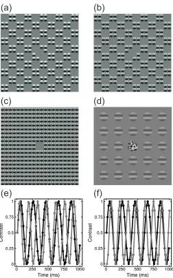
Figure 1: Example stimuli and temporal waveforms. The patterns in panels a-c are micropatches of sine-wave grating arranged in a checkerboard formation (Meese 2010). When the two components (a, b) are summed, they produce a continuous texture (c). For the binocular experiment, patches of sine-wave grating were used, with a binocular fusion lock in the center (d). Panels (e) and (f) show how stimulus contrast was temporally modulated to induce a steady-state response. The black trace in each panel is the 5Hz target modulation used in both experiments. The grey traces are the 7Hz (e) and 7.5Hz (f) mask modulations used in the space (e) and eye (f) experiments. Circles indicate the sample points used at the monitor refresh rates of 75Hz and 120Hz for the two experiments.
0 250 500 750 1000 0
0.25 0.5 0.75 1
Time (ms)
Contrast
0 250 500 750 1000 0
0.25 0.5 0.75 1
Time (ms)
Contrast
(a)
(b)
(c)
(d)
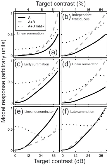
[image:3.595.172.424.270.674.2]We take this approach here, so it is the neural response to a stimulus that is of interest, which is assumed to relate in some straightforward (presumably monotonic) way to its physical properties. Consider two inputs (termed A and B) that the system wishes to combine (these could be signals from different eyes, or from adjacent locations in space, or across some arbitrary feature space, and are assumed to be monotonically related to the stimulus contrast of each input). The simplest combination rule is summation of the neural responses to the two stimuli that are linear transforms of their contrasts (resp = A + B, where resp is the overall neural response that might be measured using techniques such as MRI and EEG). Under this rule, the response to both inputs together is twice the response to either input alone (compare solid and dashed functions in Figure 2a). A similar pattern is observed for energy summation (not shown), in which the component neural responses are square-law transforms of the stimulus contrasts (Adelson and Bergen 1985). The squaring (or any other pointwise) nonlinearity alters the steepness of the function relating input contrast to output, but does not affect the ordering of the functions.
[image:4.595.318.501.74.357.2]Are these simple combination rules the ones used by the brain? For the domain of early contrast vision this seems unlikely. Even in the case where the variances of the two signals are equal (as is typically assumed within a modality), it is well established that cortical responses follow a saturating transducer nonlinearity involving contrast gain control from nearby units (Carandini and Heeger 1994, 2012). This is modelled in both single cell neurophysiology (Heeger 1992) and human psychophysics (Legge and Foley 1980) using a hyperbolic ratio function: resp = Cp / (Zq + Cq). A nonlinearity of this type will distort the summation properties of the system, yet the equation contains only a single excitatory input, the contrast (C). In principle, there are five ways in which it could be extended to accommodate multiple signals, as we now outline.
Figure 2: Predictions of six models of signal combination (panels a-f). In each panel, the model responses to a single input (A, solid curves) or two inputs (A+B, dashed curves) are compared as a function of component contrast. The dotted curves show a further condition in which a fixed signal is shown to one channel (B) and the input to the other channel (A) is increased. The individual models are described in the text. All models are normalized to the largest response at 100% input contrast across the three conditions.
Most straightforwardly, the system might sum the outputs of two individual independent transducer functions (one for each channel). This produces the pattern of responses shown in Figure 2b for canonical parameter values (p=2.4, q=2 and Z=4). The response to two inputs (A+B, dashed curve) is exactly twice the response to a single input (A, solid curve). Thus, compared with the linear model in Figure 2a, the only effect of the transducer nonlinearity is to change the shape of the functions to be less bowed on the logarithmic contrast abscissa.
Alternatively, the responses to the two inputs could be summed before they pass through the nonlinearity. This computation describes a situation where two low-amplitude signals both fall within the receptive field of a signal linear mechanism and has the equation:
0 0.5 1
1 4 16 64
A A+B A+B mask
1 4 16 64
0 0.5 1
0 0.5 1
0 12 24 36 0 12 24 36
Target contrast (dB) Target contrast (%)
Mo
d
e
l
re
sp
o
n
se
(a
rb
it
ra
ry
u
n
it
s)
(a)
(b)
(c)
(d)
(e)
(f)
Linear summation
Independent transducers
Early summation
Late summation Linear denominator
resp
=
(
A
+
B
)
pZ
q+
(
A
+
B
)
q.
(1) The predictions of this model (termed the early summation model) are shown in Figure 2c for the parameter values given above (A and B represent component contrasts). The relative increase in response when a second component is added (compare solid and dashed functions) is much smaller than for the linear and independent transducer models. This occurs because the denominator of the equation acts as a divisive gain control to normalize the two inputs (Carandini and Heeger 2012).In two further variants, either the numerator or denominator terms might be summed before exponentiation, and the others summed after exponentiation, giving rise to the models:
resp
=
(
A
+
B
)
p
Z
q+
A
q+
B
q,
(2) andresp
=
A
p
+
B
pZ
q+
(
A
+
B
)
q,
(3) with predictions shown in Figure 2d and 2e for equations 2 and 3 respectively. These models alter the relative slopes of the contrast response functions for one and two components. For the case in which inputs are summed linearly in the numerator (equation 2, Figure 2d) the response is doubled with two inputs, just as it is for the independent transducer model (Figure 2b). For linear summation in the denominator (equation 3, Figure 2e) the gain is steeper for one component (solid curve) than for two components (dashed curve) because the denominator term causes exponentially greater inhibition with two inputs. These models are similar to those proposed by Foley (1994) to explain combination of suppressive signals across stimuli of different orientations, but here we additionally consider the effect of excitatory signal combination.A final arrangement is to sum on both the numerator and denominator after exponentiation:
resp
=
A
p
+
B
pZ
q+
A
q+
B
q,
(4)The predictions for this model are shown in Figure 2f. The model predicts almost equal responses for single (A, solid curve) and double (A+B, dashed curve) inputs, particularly at high contrasts. This happens because the saturation parameter (Z) becomes negligible for large input values, and the numerator and denominator terms balance, producing a similar output for one (A) or two (A+B) inputs. In the situation where the exponents are 2 (as is often approximately the case), this model is equivalent to that proposed by Busse et al. (2009) where the RMS energy of the untuned gain pool was used as a normalization factor across orientations. The six models described above make distinct predictions about the neural response to stimuli comprising one or two components, as summarised in Figure 2. Further combinations of inputs are possible, such as fixing the contrast of one component (B) at a high level and varying the contrast of the other (A). This condition corresponds to a widely-used experimental manipulation in which a signal is shown in the presence of a constant mask. This produces the dotted curves in each plot, which are also qualitatively distinct across the different models. We therefore have a set of predictions that can be empirically tested to determine the signal combination rule used by the early visual system. We now test these predictions for steady-state EEG responses measured from human visual cortex.
2 Materials and Methods
2.1 Observers
Each experiment was completed by 12 observers of either sex, aged between 19 and 41. Five of the observers (including the author) completed both experiments in separate sessions, the remaining observers completed only one experiment each. Observers had no history of abnormal binocular vision or epilepsy, and wore their prescribed optical correction if required. We obtained written informed consent from all observers, and the study obtained ethical approval from the Department of Psychology Research Ethics Committee of the University of York.
Experiments were run on an Apple computer using a Bits# device (Cambridge Research Systems Ltd., Kent, UK), driven by code written in Matlab using the Psychtoolbox routines (Brainard 1997; Pelli 1997). In the space experiment stimuli were displayed on an Iiyama VisionMaster 510 CRT monitor running at 75Hz. In the eye experiment, stimuli were displayed on a Clinton Monoray CRT monitor running at 120Hz with stimuli presented independently to the left and right eyes using ferro-electric shutter goggles (CRS, FE-01). Both monitors were gamma corrected using a Minolta LS110 photometer.
Stimuli for the space experiment were micropattern textures made from single cycles of a 1c/deg sine-wave grating modulated by an orthogonal full-wave rectified carrier at half the spatial frequency (see Meese 2010). The micropatterns were arranged in a square grid spanning 20 carrier cycles (20 degrees). To create the ‘A’ stimulus, interdigitated checks of 2x2 micropatterns were set to 0% contrast (see Figure 1a). This arrangement was reversed to create the complementary ‘B’ stimulus (Figure 1b) such that when both A and B
components were combined they formed a continuous texture (Figure 1c). The central four micropatterns were removed to make space for a small central fixation point (black, 7 arc min wide). Stimuli flickered sinusoidally between 0% contrast and their nominal maximum contrast at combinations of 5Hz and 7Hz as shown in Figure 1e, but did not reverse in phase. The orientation of the entire pattern was randomized on each trial to prevent retinal adaptation.
Stimuli for the binocular experiment were patches of horizontal sine-wave grating two degrees in diameter, with a spatial frequency of 1c/deg. They were spatially windowed by a raised cosine envelope. The stimuli were tiled in a 5x5 grid (14 degrees in diameter), with the central grating patch omitted to make space for a cluster of dots (each 15 arc min wide) of random luminance that was used as a binocular fusion lock and fixation marker (see Figure 1d). The grid was rotated by a random amount on each trial, though the stimuli themselves remained horizontal to avoid exciting populations of neurons sensitive to horizontal carrier disparity. Stimuli flickered sinusoidally between 0% contrast
and their nominal contrast at combinations of 5Hz and 7.5Hz as shown in Figure 1f. Stimuli presented to the left eye were arbitrarily designated ‘A’ stimuli, and those presented to the right eye were ‘B’ stimuli. EEG signals were recorded at 64 electrode sites on the scalp using a WaveGuard cap (ANT Neuro, Netherlands). The EEG computer was synchronized with the display computer using an Arduino-based trigger device. Signals were amplified and digitized at 1000Hz by a PC running the ASA software (ANT Neuro, Netherlands), and stored for offline analysis.
2.3 Procedures
Participants were seated at a distance of 57cm from the display, with their chin in a rigid headrest. In the eye experiment, the goggles were attached to the headrest (rather than mounted on the head) so that they did not interfere with the EEG equipment. Stimuli were presented for trials of 11 seconds duration, with gaps of three seconds between each trial. There was no task; participants were instructed to stare at the central fixation point and avoid blinking during stimulus presentation.
Each experiment consisted of 30 different conditions, which were different pairings of
3 Results
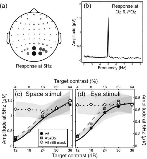
The main dependent variable was the Fourier amplitude at the target frequency (5Hz), which gave a robust signal-to-noise ratio (Figure 3b) at the occipital pole (Figure 3a). For a single component stimulus (e.g. a stimulus shown to one eye only, or to a single set of spatial locations, as in Figure 1a) the contrast response function was monotonic and showed evidence of saturation (circles in Figure 3c,d). Note that the standard errors (shaded regions) are larger at higher response levels because of individual variation in the maximum amplitude of the SSVEP response, as detailed elsewhere (Baker and Vilidaitė 2014), yet the pattern of contrast response functions we now detail was clear for individual observers.
To assess the summation properties of the system, we then flickered both components in phase at the same frequency (5Hz). Regardless of whether the stimulus was
[image:7.595.174.423.373.643.2]shown binocularly, or to both sets of spatial locations, there was very little increase in the 5Hz neural response (squares in Figure 3c,d). This is a counterintuitive finding, as the input to the system has increased by a factor of two (presumably activating many more neurons), yet the population response remains approximately constant. Models that sum stimulus contrast linearly (Figure 2a) or sum the outputs of two independent transducers (Figure 2b) entirely fail to predict this result, as do models in which components are summed before any nonlinearities on either the numerator (Figure 2d), the denominator (Figure 2e), or both (Figure 2c). However the architecture of the late summation model predicts this precise pattern (Figure 2f), which has been termed ‘ocularity invariance’ in the binocular domain (Baker et al. 2007) – the observation that the world does not change in contrast when one eye is opened or closed.
Figure 3: Results for stimuli presented at a single flicker frequency (5Hz) to assess summation properties. (a) SSVEP amplitude at 5Hz across all electrode sites, averaged across 12 observers for the ‘full’ space stimulus (Figure 1c) at 64% contrast. Circle diameter and shading are proportional to amplitude. (b) Example Fourier spectrum for the same stimulus, averaged across 12 observers and two electrode sites (Oz
and POz – the two largest circles in panela). (c) shows contrast response functions for the space stimuli when either one (circles) or two (squares) components were presented at the same flicker frequency (5Hz). The diamonds are for a condition in which one component was fixed at a high (32%) contrast, and the contrast of the other component increased. The shaded regions give ±1SE across observers (n=12). Curves are fits of the late summation model, as described in the text (fitted parameters: p=2.43, q=2.18, Z=7.46,
Rmax=0.53). (d) shows analogous contrast response functions for the eye stimuli (fitted parameters: p=2.22,
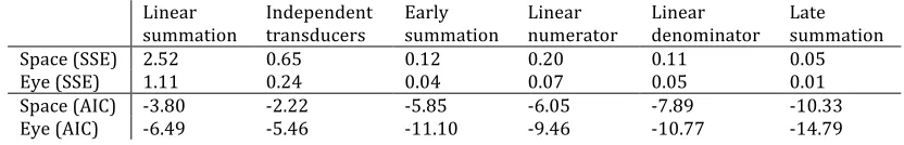
Table 1: Summed squared errors and AIC scores for six candidate models, fitted to two data sets. Smaller values indicate a better fit.
Linear summation
Independent transducers
Early summation
Linear numerator
Linear denominator
Late summation
Space (SSE) 2.52 0.65 0.12 0.20 0.11 0.05
Eye (SSE) 1.11 0.24 0.04 0.07 0.05 0.01
Space (AIC) -3.80 -2.22 -5.85 -6.05 -7.89 -10.33
Eye (AIC) -6.49 -5.46 -11.10 -9.46 -10.77 -14.79
A strong prediction of the late summation model is shown by the dotted curve in Figure 2f. This represents a condition where the B component is fixed at a high contrast (32%) and the contrast of the A component is increased. The model predicts that activity will remain constant over an intermediate range of A contrasts, despite the input to the system continually increasing. None of the other models makes this prediction, yet it is clear from the data in both experiments.
To assess which candidate model produced the best description of our results, we performed least-squares fits (downhill simplex algorithm, from 100 random starting vectors) for all six models (from Figure 2) to the data from each experiment. The linear summation model had only a single free parameter (Rmax) that multiplicatively scaled the maximum response. The other five models had four free parameters each: p, q, Z and Rmax. For both the space and binocular experiments, the late summation model gave the best numerical fit, capturing 98% and 92% of the variance within each data set respectively. The other models all produced poorer fits that explained a lower proportion of the variance, and had obvious qualitative failings. Summed squared errors and Akaike’s Information Criteria (AIC) scores that account for the number of parameters (Akaike 1974) for the six models are summarised in Table 1.
3.1 Model predictions for suppression conditions
Another manipulation available using the steady-state paradigm is to flicker the two components at different frequencies (Candy et al. 2001; Tsai et al. 2012). Responses to the two inputs can be measured independently through the early visual system (Regan and Regan 1988), permitting the isolation of suppressive processes. Figure 4a-d shows data and model predictions at the target frequency (5Hz) for
component A, when the second component (B) flickered at either 7Hz (for the space stimuli) or 7.5Hz (for the eye stimuli). Figure 4e,f shows the responses for the same conditions at the higher frequency. In each panel, the circles show the response for a single component (as in Figure 3c,d). The grey triangles (in panels a,b,e & f) show the response when both A and B
components increase in contrast together. This is equivalent to the grey squares in Figure 3, but now flickering at different frequencies. Note that the grey triangle function in all panels is shallower than the single component (circle) function, showing the effect of suppression on the gain of the system. This demonstrates the action of the inhibitory terms in the denominator of equation 4.
The white inverted triangles in Figure 4c-f represent the condition in which a high contrast (32%) mask stimulus is shown at the higher frequency. The target contrast at the lower frequency (5Hz) is increased along the abscissa. The white triangle contrast response function in Figure 4c,d is shifted to the right relative to the single component (circles) function. This is a classic contrast gain control effect, reported widely in previous human SSVEP (Candy et al. 2001; Busse et al. 2009; Tsai et al. 2012; Baker and Vilidaitė 2014), animal SSVEP (Afsari et al. 2014) and single-cell (Morrone et al. 1982; Carandini and Heeger 1994) studies. The white inverted triangles in Figure 4e,f show the complementary response at the mask frequency as target contrast increases. There is a reduction in response at higher target contrasts, showing the suppressive effect of the target on the mask.
[image:8.595.86.502.93.160.2](presumably involving the same populations of neurons as when a single component is presented at that frequency), giving,
resp
=
A
p
Z
q+
A
q+
B
q.
(5)Importantly, we fixed the parameters at the fitted values from Figure 3. With no free parameters, the model correctly predicted the form of the data in Figure 4a-e. Because responses were reduced slightly at 7.5Hz, we permitted Rmax to vary (it reduced from 0.71 to 0.53) in order to better fit the data in Figure 4f.
Figure 4: Panels (a,b,c,d) show SSVEP responses at the target frequency (5Hz) when the mask (B component) flickered at a higher frequency (7Hz for the space condition (a,c); 7.5Hz for the eye condition (b,d)). Panels (e,f) show SSVEP responses at the mask frequency (7 or 7.5Hz) when the target flickered either at 7/7.5Hz (circles) or at 5Hz (with a mask at the higher frequency). In each panel the shaded regions indicate ±1SE of the mean of each data point. The curves are predictions of the late summation model with no free parameters (except in panel f, where Rmax was permitted to vary).
The model explained 89% (space) and 73% (eye) of the variance in these extra conditions. The poorer fit for the eye data is mostly due to a shallower-than-predicted contrast response function in Figure 4d (inverted triangles). This resembles a
response gain effect (e.g. a change in Rmax) rather than a contrast gain effect (see Li et al. 2005), and we are actively investigating this discrepancy in a further study. It is possible that a more sophisticated multi-stage model (Meese et al. 2006) would give a better description of the binocular data. However, despite this shortcoming, the model correctly predicts the differences in gradient of the contrast response functions in all panels of Figure 4. Overall, we can capture the pattern of eight contrast response functions (40 data points) for two distinct stimulus domains with only four free parameters. This illustrates the generality and predictive power of the model.
3.2 Model predictions for harmonic and intermodulation frequencies
[image:9.595.93.280.281.540.2]Presentation of two frequencies simultaneously produced evoked responses at sums and differences of the fundamentals, as has been reported previously (Tsai et al. 2012). These can be seen in the empirical and model spectra shown in Figure 5c,d (highlighted green), and as a function of contrast for one condition in the surface plots of Figure 6. A novel observation is that responses are also evoked at specific additional frequencies that appear to be combinations of fundamental, harmonic and intermodulation terms (e.g. 3, 4, 8, 9, 16, 18 and 19Hz all had SNR>2). The model also produces responses at most of these frequencies (Figure 5d), though the signals are sometimes stronger (e.g. 12Hz) and sometimes weaker (e.g. 14Hz) than those found in the empirical data. We suspect that these discrepancies might indicate the presence of neurons that involve further nonlinear stages of processing. Examples include complex cells that code changes in
contrast (which might account for the increased second harmonic responses) and conjunction detectors (AND gates). We intend to model these cell types explicitly in future, though doing so is beyond the scope of the present study.
[image:10.595.159.435.369.634.2]We also attempted fitting the model to the entire spectrum from 1-30Hz across all conditions. This produced similar parameter values to those described above, and comparable fits to the contrast response functions at fundamental frequencies, but additionally gave a good account of responses at harmonic, intermodulation and other integer frequencies. The model was able to account for 69% of the variance of each of the space and eye data sets, with each data set consisting of 8730 data points (30 conditions by 291 frequencies in steps of 0.1Hz). With only four free parameters, this seems an impressive performance.
4 Discussion
[image:11.595.91.291.340.632.2]We tested the predictions of six models of cortical signal combination for two visual stimulus domains (space and eye-of-origin). We found that the late summation model (equation 4) correctly captured the pattern of contrast response functions for three conditions (Figure 3c,d) and predicted several other conditions with no free parameters (Figures 4a-c, 5c,d and 6). Alternative models that sum individual channel responses before nonlinear transduction failed to correctly describe the pattern of results. We discuss the implications of these findings for our understanding of the relationship between perception and neural activity, and speculate that the preferred model of contrast normalization is a neural implementation of Bayes-optimal signal combination.
Figure 6: Surface plots showing empirical (a) and model (b) signal-to-noise ratios as a function of frequency (left abscissa) and contrast (right abscissa). The condition was the A5+B7 mask condition from the space experiment, in which the 7Hz mask component had a fixed contrast of 32%, and the 5Hz target component contrast increased along the right abscissa. The blue-highlighed functions indicate the target frequency (5Hz) and its harmonics. The red-highlighted functions indicate the mask frequency (7Hz) and its harmonics.
Green-highlighted functions indicate the intermodulation frequencies (7-5=2 and 7+5=12Hz). In the human data, the higher harmonics produce relatively larger amplitudes than in the model. Model parameters are given in the caption to Figure 3.
4.1 Perception and neural activity
A body of recent psychophysical work has converged on the same algorithm for signal combination that we are proposing in this study (Meese and Baker 2013). These studies used a range of detection, discrimination and matching paradigms to investigate the perception of stimuli summed across dimensions such as eye (Meese et al. 2006; Baker et al. 2007), space (Meese and Summers 2007), time and orientation (Meese and Baker 2013). Our results demonstrate that this model is consistent with the pattern of cortical responses at a population level, and other work has converged on a similar algorithm for binocular combination using fMRI (Moradi and Heeger 2009) and for combination across orientation in neural populations (Busse et al. 2009). Such consistency across measurement techniques is extremely unusual, and implies that the model is an accurate reflection of the operations performed by the brain in combining signals.
In general, there is no reason to think that the model proposed here applies only to vision, or to the specific visual dimensions explored (space and eye-of-origin). We have shown already that the same algorithm applies equally well to psychophysical summation across orientation and time (Baker et al. 2013; Meese and Baker 2013). Furthermore, a strikingly similar model has been proposed for explaining neural population responses to stimuli of different orientations (Busse et al. 2009). That model involved subtle differences in the way that suppressive signals are pooled (computing the RMS contrast), but fitted the present data almost as well as the preferred model here (not shown). The models can be considered architecturally equivalent, supporting the idea that common operations apply within distinct visual cues. Given the ubiquity of canonical microcircuits and computations, such as gain control (Carandini and Heeger 2012), it is conceivable that the same algorithm will be implemented at higher levels of the visual system and in other senses. Likely candidates are binaural and cross-frequency combination in hearing (Treisman 1967), and spatial summation across the skin for vibration (Haggard and Giovagnoli 2011). In high level vision, there is evidence that information is pooled across objects such as faces (Young et al. 1987; Boremanse et al. 2013). In principle these operations might be achieved by the same computations that are used for combining simpler visual features.
4.2 At what level is the algorithm implemented?
Steady-state EEG is believed to measure aggregate responses across large populations of neurons (most likely pyramidal cells in the superficial layers of cortex) that are responsive to a given stimulus (Norcia et al. 2015). This population response will likely encompass neurons with differential weightings across the two inputs (in the binocular case, different levels of ocular dominance, and in the spatial case, different receptive field positions or shapes), as well as a range of contrast sensitivities, that we do not model explicitly here (for further discussion, see Busse et al. 2009). As such, the model we propose can be thought of as representing an omnibus population response, rather
than the activity of individual cells, in a manner similar to the fMRI BOLD response. From the perspective of David Marr’s framework (Marr 1983), the models described here are therefore algorithm-level explanations of signal combination, rather than implementation-level explanations (i.e. circuit diagrams) that would make assumptions about synaptic connections between neurons, specific classes of cell involved, or numbers of cells responding to a particular stimulus. In principle the basic algorithm could be implemented in any number of ways, and we expect that single-cell neurophysiology might reveal how this is achieved in cortex.
In psychophysical studies that have used similar stimuli (Meese et al. 2006; Meese and Summers 2007; Meese and Baker 2013), observers are assumed to base their responses on the activity of a small number of neurons most appropriate for the task at hand, and make discriminations within a signal detection theory framework (i.e. choosing the interval that produces the largest response after combination with additive internal noise). That the algorithm presented here is also able to give a good account of such data suggest that the combination rules are sufficiently generic that they apply across the whole population of neurons.
4.3 Optimal signal combination
Equation 4 can be straightforwardly rewritten as,
(6) where the weight terms (ωA, ωB) are implicitly set to unity. This bears a striking similarity to the optimal combination rule for two inputs (Ernst and Bülthoff 2004), which is a Kalman filter (Kalman and Bucy 1961). The static filter gain (L) is given by:
L= σA
2
PA σA2σ
B 2
+σA2
PA+σB 2
PB
σB
2
PB σB2σ
A 2
+σB2
PB+σA 2
PA
⎡
⎣
⎢ ⎤
⎦ ⎥,
(7) where PA is the response of the channel (or sensor) tuned to input A, and σA2 is the variance, with terms bearing the subscript B
by the inverse of its contribution to the total variance. This filter has numerous applications in engineering, including the fusion of image data from multiple sensors (e.g. Willner et al. 1976). For the situation where the two inputs have equal variance (i.e. the two eyes) the weight terms are immaterial, and the filter becomes similar to our model. In the hypothetical case where the numerator and denominator exponents are equal (as we found for binocular combination, see Figure 3) and P represents contrast energy (A2 and B2), the two models
become identical. We therefore speculate that combination within a cue might be statistically optimal as a consequence of divisive normalization. We also note that dynamic (time-dependent) Kalman filters include the history of recent inputs in calculating the weights, a computation that has obvious parallels with contrast adaptation (Carandini and Ferster 1997) and attention (Reynolds and Heeger 2009), both of which are closely related to gain control.
Previous models that implement optimal cue combination have focused on cases where the two inputs are from different modalities (e.g. vision and touch, Ernst and Banks 2002) that have unequal variances. Indeed one recent study developed a normalization model with the same general form as that we propose here to account for several specific multisensory integration phenomena in neurons in the superior colliculus and area MSTd (Ohshiro et al. 2011). Yet so far a theoretical link between normalization and optimal signal combination has remained elusive: as Ohshiro et al. (2011) explicitly state, "It is currently unclear what roles divisive normalization may have in a theory of optimal cue integration and this is an important topic for additional investigation." We speculate here that gain control suppression may be the mechanism by which signals are weighted to permit their optimal combination. The exponent values in equation 6 are presumably a consequence of the neural implementation of this weighting principle.
To our knowledge, this is a novel account of the purpose of cortical gain control, which is a canonical neural operation observed throughout the brain (Carandini and Heeger 2012). In addition, it makes clear predictions for situations in which one input
is noisier than the other. A natural example for binocular vision is amblyopia, in which the amblyopic eye’s responses are both weaker (i.e. suppressed) (Baker et al. 2008, 2015) and noisier (Levi and Klein 2003; Baker et al. 2008) than those of the fellow eye. Previously, the increased noise has been considered secondary to the suppression. But our account suggests that the amblyopic suppression might be a Bayes-optimal consequence of one input being noisier (perhaps because of erratic fixation due to strabismus) than the other during development. This might explain why attempts to reduce the suppression by increasing noise in the fellow eye appear to be successful (Hess et al. 2010).
4.4 Conclusions
A single, simple algorithm was shown to accurately predict a complex pattern of steady-state contrast response functions for signal combination across space and eye. This algorithm is a strong candidate for a canonical model of optimal neural signal combination, and may well be relevant in senses other than vision, and perhaps throughout the cerebral cortex more generally. Because the same model can explain both steady-state EEG and psychophysical data, it highlights the close link between perception and neural activity. By suggesting that gain control suppression implements optimal signal combination, we have shown how two of the most influential concepts in modern neuroscience (contrast gain control (Heeger 1992; Carandini and Heeger 2012) and Bayesian information theory (Ernst and Bülthoff 2004; Friston 2010)) might be unified.
5 Funding
This work was supported by the Wellcome Trust (grant number 105624) through the Centre for Chronic Diseases and Disorders (C2D2) at the University of York (to DHB); the Royal Society (grant number RG130121 to DHB); and the European Research Council Marie Curie (grant number RE223301 to ARW).
6 Acknowledgements
7 References
Adelson EH, Bergen JR. 1985. Spatiotemporal energy models for the perception of motion. J Opt Soc Am A. 2:284–299.
Afsari F, Christensen KV, Smith GP, Hentzer M, Nippe OM, Elliott CJH, Wade AR. 2014. Abnormal visual gain control in a Parkinson’s disease model. Hum Mol Genet. 23:4465– 4478.
Akaike H. 1974. A new look at the statistical model identification. IEEE Transactions on Automatic Control. 19:716–723.
Baker DH, Meese TS, Georgeson MA. 2007. Binocular interaction: contrast matching and contrast discrimination are predicted by the same model. Spatial Vision. 20:397–413. Baker DH, Meese TS, Georgeson MA. 2013.
Paradoxical psychometric functions (“swan functions”) are explained by dilution masking in four stimulus dimensions. Iperception. 4:17–35.
Baker DH, Meese TS, Hess RF. 2008. Contrast masking in strabismic amblyopia: attenuation, noise, interocular suppression and binocular summation. Vision Res. 48:1625–1640.
Baker DH, Simard M, Saint-Amour D, Hess RF. 2015. Steady-state contrast response functions provide a sensitive and objective index of amblyopic deficits. Investigative Ophthalmology & Visual Science.
Baker DH, Vilidaitė G. 2014. Broadband noise masks suppress neural responses to narrowband stimuli. Front Psychol. 5:763. Blakemore C, Campbell FW. 1969. On the
existence of neurones in the human visual system selectively sensitive to the orientation and size of retinal images. J Physiol. 203:237– 260.
Boremanse A, Norcia AM, Rossion B. 2013. An objective signature for visual binding of face parts in the human brain. Journal of Vision. 13:6–6.
Brainard DH. 1997. The Psychophysics Toolbox. Spat Vis. 10:433–436.
Busse L, Wade AR, Carandini M. 2009. Representation of Concurrent Stimuli by Population Activity in Visual Cortex. Neuron. 64:931–942.
Candy TR, Skoczenski AM, Norcia AM. 2001. Normalization models applied to orientation masking in the human infant. J Neurosci. 21:4530–4541.
Carandini M, Ferster D. 1997. A Tonic Hyperpolarization Underlying Contrast Adaptation in Cat Visual Cortex. Science. 276:949–952.
Carandini M, Heeger DJ. 1994. Summation and division by neurons in primate visual cortex. Science. 264:1333–1336.
Carandini M, Heeger DJ. 2012. Normalization as a canonical neural computation. Nat Rev Neurosci. 13:51–62.
Derrington AM, Lennie P. 1984. Spatial and temporal contrast sensitivities of neurones in lateral geniculate nucleus of macaque. J Physiol (Lond). 357:219–240.
Einicke G. 2012. Nonlinear Prediction, Filtering and Smoothing. In: A. G, editor. Smoothing, Filtering and Prediction - Estimating The Past, Present and Future. InTech.
Ernst MO, Banks MS. 2002. Humans integrate visual and haptic information in a statistically optimal fashion. 429–433.
Ernst MO, Bülthoff HH. 2004. Merging the senses into a robust percept. Trends in Cognitive Sciences. 8:162–169.
Foley JM. 1994. Human luminance pattern-vision mechanisms: masking experiments require a new model. J Opt Soc Am A. 11:1710–1719. Freeman J, Ziemba CM, Heeger DJ, Simoncelli EP,
Movshon JA. 2013. A functional and perceptual signature of the second visual area in primates. Nat Neurosci. 16:974–981. Friston K. 2010. The free-energy principle: a
unified brain theory? Nature Reviews Neuroscience. 11:127–138.
Georgeson MA, May KA, Freeman TCA, Hesse GS. 2007. From filters to features: Scale-space analysis of edge and blur coding in human vision. Journal of Vision. 7:(13): 7.
Gheorghiu E, Kingdom FAA. 2008. Spatial properties of curvature-encoding mechanisms revealed through the shape-frequency and shape-amplitude after-effects. Vision Res. 48:1107–1124.
Haggard P, Giovagnoli G. 2011. Spatial patterns in tactile perception: Is there a tactile field? Acta Psychologica. 137:65–75.
Heeger DJ. 1992. Normalization of cell responses in cat striate cortex. Vis Neurosci. 9:181–197. Hess RF, Mansouri B, Thompson B. 2010. A
binocular approach to treating amblyopia: antisuppression therapy. Optom Vis Sci. 87:697–704.
Hubel DH, Wiesel TN. 1959. Receptive fields of single neurones in the cat’s striate cortex. J Physiol. 148:574–591.
Kalman RE, Bucy RS. 1961. New results in linear filtering and prediction theory. Journal of Basic Engineering. 83:95–108.
Kay KN, Winawer J, Mezer A, Wandell BA. 2013. Compressive spatial summation in human visual cortex. Journal of Neurophysiology. 110:481–494.
Kay KN, Winawer J, Rokem A, Mezer A, Wandell BA. 2013. A Two-Stage Cascade Model of BOLD Responses in Human Visual Cortex. PLoS Computational Biology. 9:e1003079. Legge GE, Foley JM. 1980. Contrast masking in
human vision. J Opt Soc Am. 70:1458–1471. Levi DM, Klein SA. 2003. Noise provides some
new signals about the spatial vision of amblyopes. J Neurosci. 23:2522–2526. Li B, Peterson MR, Thompson JK, Duong T,
Suppression: Monoptic and Dichoptic Mechanisms Are Different. Journal of Neurophysiology. 94:1645–1650.
Marr D. 1983. Vision: A Computational Investigation into the Human Representation and Processing of Visual Information. W. H. Freeman.
Meese TS. 2010. Spatially extensive summation of contrast energy is revealed by contrast detection of micro-pattern textures. J Vis. 10:14: 1–21.
Meese TS, Baker DH. 2013. A common rule for integration and suppression of luminance contrast across eyes, space, time, and pattern. Iperception. 4:1–16.
Meese TS, Georgeson MA, Baker DH. 2006. Binocular contrast vision at and above threshold. J Vis. 6:1224–1243.
Meese TS, Summers RJ. 2007. Area summation in human vision at and above detection threshold. Proc R Soc Lond B Biol Sci. 274:2891–2900.
Moradi F, Heeger DJ. 2009. Inter-ocular contrast normalization in human visual cortex. J Vis. 9:13.1–22.
Morrone MC, Burr DC, Maffei L. 1982. Functional implications of cross-orientation inhibition of cortical visual cells. I. Neurophysiological evidence. Proc R Soc Lond B Biol Sci. 216:335–354.
Norcia AM, Appelbaum LG, Ales JM, Cottereau BR, Rossion B. 2015. The steady-state visual evoked potential in vision research: A review. Journal of Vision. 15(6):4:1–46.
Ohshiro T, Angelaki DE, DeAngelis GC. 2011. A normalization model of multisensory
integration. Nature Neuroscience. 14:775– 782.
Peirce JW. 2015. Understanding mid-level representations in visual processing. Journal of Vision. 15:5.
Pelli DG. 1997. The VideoToolbox software for visual psychophysics: transforming numbers into movies. Spat Vis. 10:437–442.
Regan MP, Regan D. 1988. A frequency domain technique for characterizing nonlinearities in biological systems. Journal of Theoretical Biology. 133:293–317.
Reynolds JH, Heeger DJ. 2009. The Normalization Model of Attention. Neuron. 61:168–185. Robson JG, Graham N. 1981. Probability
summation and regional variation in contrast sensitivity across the visual field. Vision Res. 21:409–418.
Tootell RB, Switkes E, Silverman MS, Hamilton SL. 1988. Functional anatomy of macaque striate cortex. II. Retinotopic organization. J Neurosci. 8:1531–1568.
Treisman M. 1967. Auditory Intensity Discriminal Scale I. Evidence Derived from Binaural Intensity Summation. The Journal of the Acoustical Society of America. 42:586. Tsai JJ, Wade AR, Norcia AM. 2012. Dynamics of
normalization underlying masking in human visual cortex. J Neurosci. 32:2783–2789. Willner D, Chang C, Dunn K. 1976. Kalman filter
algorithms for a multi-sensor system. IEEE. p. 570–574.