GOODS-ALMA: 1.1 mm galaxy survey I. Source catalog and optically dark galaxies

optically dark galaxies

.

White Rose Research Online URL for this paper:

http://eprints.whiterose.ac.uk/140675/

Version: Published Version

Article:

Franco, M., Elbaz, D., Bethermin, M. et al. (36 more authors) (2018) GOODS-ALMA: 1.1

mm galaxy survey I. Source catalog and optically dark galaxies. Astronomy and

Astrophysics, 620. A152. ISSN 0004-6361

https://doi.org/10.1051/0004-6361/201832928

Reproduced with permission from Astronomy & Astrophysics, © ESO

eprints@whiterose.ac.uk https://eprints.whiterose.ac.uk/

Reuse

Items deposited in White Rose Research Online are protected by copyright, with all rights reserved unless indicated otherwise. They may be downloaded and/or printed for private study, or other acts as permitted by national copyright laws. The publisher or other rights holders may allow further reproduction and re-use of the full text version. This is indicated by the licence information on the White Rose Research Online record for the item.

Takedown

If you consider content in White Rose Research Online to be in breach of UK law, please notify us by

https://doi.org/10.1051/0004-6361/201832928 c

ESO 2018

Astronomy

&

Astrophysics

GOODS-ALMA: 1.1 mm galaxy survey

I. Source catalog and optically dark galaxies

M. Franco

_{, D. Elbaz}

_{, M. Béthermin}

_{, B. Magnelli}

_{, C. Schreiber}

_{, L. Ciesla}

_{, M. Dickinson}

_{, N. Nagar}

_,

J. Silverman

_{, E. Daddi}

_{, D. M. Alexander}

_{, T. Wang}

_{, M. Pannella}

_{, E. Le Floc’h}

_{, A. Pope}

_{, M. Giavalisco}

_,

A. J. Maury

_{, F. Bournaud}

_{, R. Chary}

_{, R. Demarco}

_{, H. Ferguson}

_{, S. L. Finkelstein}

_{, H. Inami}

_{, D. Iono}

_,

S. Juneau

_{, G. Lagache}

_{, R. Leiton}

_{, L. Lin}

_{, G. Magdis}

_{, H. Messias}

_{, K. Motohara}

_{, J. Mullaney}

_,

K. Okumura

_{, C. Papovich}

_{, J. Pforr}

_{, W. Rujopakarn}

_{, M. Sargent}

_{, X. Shu}

_{, and L. Zhou}

(Affiliations can be found after the references)

Received 1 March 2018/Accepted 30 July 2018

ABSTRACT

Aims.We present a 69 arcmin2ALMA survey at 1.1 mm, GOODS-ALMA, matching the deepest HST-WFC3H-band part of the GOODS-South

field.

Methods.We tapered the 0′′_{24 original image with a homogeneous and circular synthesized beam of 0}′′_{60 to reduce the number of independent}

beams – thus reducing the number of purely statistical spurious detections – and optimize the sensitivity to point sources. We extracted a catalog of galaxies purely selected by ALMA and identified sources with and without HST counterparts down to a 5σlimiting depth ofH=28.2 AB (HST/WFC3 F160W).

Results.ALMA detects 20 sources brighter than 0.7 mJy at 1.1 mm in the 0′′_{60 tapered mosaic (rms sensitivityσ≃0.18 mJy beam}−1_{) with}

a purity greater than 80%. Among these detections, we identify three sources with no HST norSpitzer-IRAC counterpart, consistent with the expected number of spurious galaxies from the analysis of the inverted image; their definitive status will require additional investigation. We detect additional three sources with HST counterparts either at high significance in the higher resolution map, or with different detection-algorithm

parameters ensuring a purity greater than 80%. Hence we identify in total 20 robust detections.

Conclusions.Our wide contiguous survey allows us to push further in redshift the blind detection of massive galaxies with ALMA with a median

redshift ofz=2.92 and a median stellar mass ofM⋆=1.1×1011M⊙. Our sample includes 20% HST-dark galaxies (4 out of 20), all detected

in the mid-infrared withSpitzer-IRAC. The near-infrared based photometric redshifts of two of them (z_∼4.3 and 4.8) suggest that these sources have redshiftsz>4. At least 40% of the ALMA sources host an X-ray AGN, compared to_∼14% for other galaxies of similar mass and redshift. The wide area of our ALMA survey provides lower values at the bright end of number counts than single-dish telescopes affected by confusion.

Key words. galaxies: high-redshift – galaxies: evolution – galaxies: star formation – galaxies: active – galaxies: photometry –

submillimeter: galaxies

1. Introduction

In the late 1990s a population of galaxies was discovered at submillimeter wavelengths using the Submillimeter

Common-User Bolometer Array (SCUBA; Holland et al. 1999) on the

James Clerk Maxwell Telescope (see e.g., Smail et al. 1997;

Hughes et al. 1998;Barger et al. 1998;Blain et al. 2002). These “submillimeter galaxies” or SMGs are highly obscured by

dust, typically located around z _∼ 2–2.5 (e.g., Chapman et al.

2003; Wardlow et al. 2011; Yun et al. 2012), massive (M⋆ >

7 ×1010M_⊙; e.g., Chapman et al. 2005; Hainline et al. 2011;

Simpson et al. 2014), gas-rich (fgas > 50%; e.g., Daddi et al.

2010), with huge star formation rates (SFR) – often greater

than 100M_⊙yr−1 _{(e.g., Magnelli et al. 2012; Swinbank et al.}

2014) – making them significant contributors to the cosmic

star formation (e.g.,Casey et al. 2013), often driven by mergers

(e.g.,Tacconi et al. 2008;Narayanan et al. 2010) and often host

an active galactic nucleus (AGN; e.g., Alexander et al. 2008;

Pope et al. 2008; Wang et al. 2013). These SMGs are plausi-ble progenitors of present-day massive early-type galaxies (e.g.,

Cimatti et al. 2008;Michałowski et al. 2010).

Recently, thanks to the advent of the Atacama Large

Mil-limeter/submillimeter Array (ALMA) and its capabilities to

perform both high-resolution and high-sensitivity observations, our view of SMGs has become increasingly refined. The high angular resolution compared to single-dish observations reduces drastically the uncertainties of source confusion and

blend-ing, and affords new opportunities for robust galaxy

identifica-tion and flux measurement. The ALMA sensitivity allows for

the detection of sources down to 0.1 mJy (e.g.,Carniani et al.

2015), the analysis of populations of dust-poor high-z

galax-ies (Fujimoto et al. 2016) or main sequence (MS;Noeske et al.

2007; Rodighiero et al. 2011; Elbaz et al. 2011) galaxies (e.g.,

Papovich et al. 2016;Dunlop et al. 2017;Schreiber et al. 2017), and also demonstrates that the extragalactic background light (EBL) can be resolved partially or totally by faint

galax-ies (S < 1 mJy; e.g.,Hatsukade et al. 2013; Ono et al. 2014;

Carniani et al. 2015; Fujimoto et al. 2016). Thanks to this new domain of sensitivity, ALMA is able to unveil less extreme objects, bridging the gap between massive starbursts and more normal galaxies: SMGs no longer stand apart from the general galaxy population.

unbiased view of a large (69 arcmin2_{) region of the sky,}

with-out prior or a posteriori selection based on already known galax-ies, in order to improve our understanding of dust-obscured star formation and investigate the main properties of these objects. We take advantage of one of the most uncertain and poten-tially transformational outputs of ALMA – its ability to reveal a new class of galaxies through serendipitous detections. This is one of the main reasons for performing blind extragalactic surveys.

Thanks to the availability of very deep, panchromatic pho-tometry at rest-frame UV, optical and NIR in legacy fields such as great observatories origins deep survey-South (GOODS-South), which also includes among the deepest available X-ray and radio maps, precise multiwavelength analysis that include the crucial FIR region is now possible with ALMA. In

partic-ular, a population of high redshift (2 < z < 4) galaxies, too

faint to be detected in the deepest HST-WFC3 images of the GOODS-South field has been revealed, thanks to the thermal dust emission seen by ALMA. Sources without an HST

coun-terpart in theH-band, the reddest available (so-called HST-dark)

have been previously found by color selection (e.g.,Huang et al.

2011;Caputi et al. 2012,2015;Wang et al. 2016), by

serendip-itous detection of line emitters (e.g.,Ono et al. 2014) or in the

continuum (e.g.,Fujimoto et al. 2016). We will show that_∼20%

of the sources detected in the survey described in this paper are HST-dark, and strong evidence suggests that they are not spuri-ous detections.

The aim of the work presented in this paper is to

exploit a 69 arcmin2 _{ALMA image reaching a sensitivity of}

0.18 mJy at a resolution of 0′′_{60. We used the leverage of}

the excellent multiwavelength supporting data in the GOODS-South field: the cosmic assembly near-infrared deep

extra-galactic legacy survey (Koekemoer et al. 2011; Grogin et al.

2011), the Spitzer extended deep survey (Ashby et al. 2013),

the GOODS-Herschelsurvey (Elbaz et al. 2011), theChandra

deep field-South (Luo et al. 2017) and ultra-deep radio

imag-ing with the VLA (Rujopakarn et al. 2016), to construct a robust

catalog and derive physical properties of ALMA-detected galax-ies. The region covered by ALMA in this survey corre-sponds to the region with the deepest HST-WFC3 coverage, and has also been chosen for a guaranteed time

observa-tion (GTO) program with the James Webb Space Telescope

(JWST).

This paper is organized as follows: in Sect.2 we describe

our ALMA survey, the data reduction, and the

multiwave-length ancillary data which support our studies. In Sect.3, we

present the methodology and criteria used to detect sources, we also present the procedures used to compute the

complete-ness and the fidelity of our flux measurements. In Sect. 4 we

detail the different steps we conducted to construct a

cata-log of our detections. In Sect. 5 we estimate the differential

and cumulative number counts from our detections. We

com-pare these counts with other (sub)millimeter studies. In Sect.6

we investigate some properties of our galaxies such as red-shift and mass distributions. Other properties will be analyzed

in Franco et al. (in prep.) and finally in Sect. 8, we

summa-rize the main results of this study. Throughout this paper, we

adopt a spatially flat ΛCDM cosmological model with H0 =

70 kms−1_Mpc−1_{,Ωm=0.7 andΩΛ=0.3. We assume a Salpeter}

(Salpeter 1955) initial mass function (IMF). We used the

con-version factor ofM⋆(Salpeter 1955, IMF)=1.7×M⋆(Chabrier

2003, IMF). All magnitudes are quoted in the AB system

(Oke & Gunn 1983).

2. ALMA GOODS-South survey data

2.1. Survey description

Our ALMA coverage extends over an effective area of

69 arcmin2 _{within the GOODS-South field (Fig. 1), centered}

atα = 3h32m30.0s,δ = ₋27◦₄₈′₀₀′′ _{(J2000; 2015.1.00543.S;}

PI: D. Elbaz). To cover this _∼10′_×7′ _{region (comoving scale}

of 15.1 Mpc×10.5 Mpc atz =2), we designed a 846-pointing

mosaic, each pointing being separated by 0.8 times the antenna

half power beam width (HPBW∼23′′_3).

To accommodate such a large number of pointings within the ALMA Cycle 3 observing mode restrictions, we divided this mosaic into six parallel, slightly overlapping, submosaics of 141 pointing each. To get a homogeneous pattern over the 846

point-ings, we computed the offsets between the submosaics so that

they connected with each other without breaking the hexagonal pattern of the ALMA mosaics.

Each submosaic (or slice) had a length of 6.8 arcmin, a width

of 1.5 arcmin and an inclination (PA) of 70 deg (see Fig.1). This

required three execution blocks (EBs), yielding a total on-source

integration time of∼60 s per pointing (Table1). We determined

that the highest frequencies of the band 6 were the optimal setup for a continuum survey and we thus set the ALMA correlator to Time Division Multiplexing (TDM) mode and optimized the

setup for continuum detection at 264.9 GHz (λ=1.13 mm) using

four 1875 MHz-wide spectral windows centered at 255.9 GHz, 257.9 GHz, 271.9 GHz and 273.9 GHz, covering a total

band-width of 7.5 GHz. The TDM mode has 128 channels per spectral

window, providing us with_∼37 km s−1_{velocity channels.}

Observations were taken between the 1st of August and the

2nd of September 2016, using_∼40 antennae (see Table1) in

con-figuration C40-5 with a maximum baseline of_∼1500 m. J0334–

4008 and J0348–2749 (VLBA calibrator and hence has a highly precise position) were systematically used as flux and phase cal-ibrators, respectively. In 14 EBs, J0522–3627 was used as

band-pass calibrator, while in the remaining 4 EBs J0238+1636 was

used. Observations were taken under nominal weather

condi-tions with a typical precipitable water vapor of_∼1 mm.

2.2. Data reduction

All EBs were calibrated with CASA (McMullin et al. 2007)

using the scripts provided by the ALMA project. Calibrated visibilities were systematically inspected and few additional flaggings were added to the original calibration scripts. Flux calibrations were validated by verifying the accuracy of our phase and bandpass calibrator flux density estimations. Finally, to reduce computational time for the forthcoming continuum imaging, we time- and frequency-averaged our calibrated EBs over 120 s and 8 channels, respectively.

Imaging was done in CASA using the multifrequency

syn-thesis algorithm implemented within the task CLEAN.

Submo-saics were produced separately and combined subsequently using a weighted mean based on their noise maps. As each

submosaic was observed at different epochs and under diff

er-ent weather conditions, they exhibit different synthesized beams

and sensitivities (Table1). Submosaics were produced and

pri-mary beam corrected separately, to finally be combined using a weighted mean based on their noise maps. To obtain a relatively homogeneous and circular synthesized beam across our final

mosaic, we applied differentu,vtapers to each submosaic. The

best balance between spatial resolution and sensitivity was found

Fig. 1.ALMA 1.1 mm image tapered at 0′′_{60. The white circles have a diameter of 4 arcseconds and indicate the positions of the galaxies listed}

in Table3. Black contours show the different slices (labeled A–F) used to compose the homogeneous 1.1 mm coverage, with a median

rms-noise of 0.18 mJy per beam. Blue lines show the limits of the HST/ACS field and green lines indicate the HST-WFC3 deep region. The cyan

contour represents the limit of theDunlop et al.(2017) survey covering all theHubbleUltra Deep Field region. All of the ALMA-survey field is encompassed by theChandradeep field-South.

width half maximum (FWHM; hereafter 0′′_{29-mosaic; Table1).}

This resolution corresponds to the highest resolution for which a circular beam can be synthesized for the full mosaic. We also applied this tapering method to create a second mosaic with a

homogeneous and circular synthesized beam of 0′′_{60 FWHM}

(hereafter 0′′_{60-mosaic; Table1), in other words, optimized for}

the detection of extended sources. Mosaics with even coarser spatial resolution could not be created because of drastic sensi-tivity and synthesized beam shape degradations.

Due to the good coverage in theuv-plane (see Fig.2) and the

absence of very bright sources (the sources present in our image

do not cover a large dynamic range in flux densities; see Sect.4),

we decided to work with the dirty map. This prevents introducing

potential biases during theCLEANprocess and we noticed that the

noise in the clean map is not significantly different (<1%).

2.3. Building of the noise map

We built the rms-map of the ALMA survey by a k-σclipping

method. In steps of four pixels on the image map, the

stan-dard deviation was computed in a square of 100×100 pixels

around the central pixel. The pixels, inside this box, with

val-ues greater than three times the standard deviation (σ) from the

median value were masked. This procedure was repeated three times. Finally, we assigned the value of the standard deviation

of the non-masked pixels to the central pixel. This box size cor-responds to the smallest size for which the value of the median pixel of the rms map converges to the typical value of the noise in the ALMA map while taking into account the local variation of noise. The step of four pixels corresponds to a subsampling of the beam so, the noise should not vary significantly on this scale.

The median value of the standard deviation is 0.176 mJy beam−1_.

In comparison, the Gaussian fit of the unclipped map gave a

stan-dard deviation of 0.182 mJy beam−1_{. We adopted a general value}

of rms sensitivityσ=0.18 mJy beam−1_{. The average values for}

the 0′′_{29-mosaic and the untapered mosaic are given in Table1.}

2.4. Ancillary data

The area covered by this survey is ideally located, in that it prof-its from ancillary data from some of the deepest sky surveys at infrared (IR), optical and X-ray wavelengths. In this section, we describe all of the data that were used in the analysis of the ALMA detected sources in this paper.

2.4.1. Optical and near-infrared imaging

We have supporting data from the Cosmic Assembly Near-IR

Deep Extragalactic Legacy Survey (CANDELS; Grogin et al.

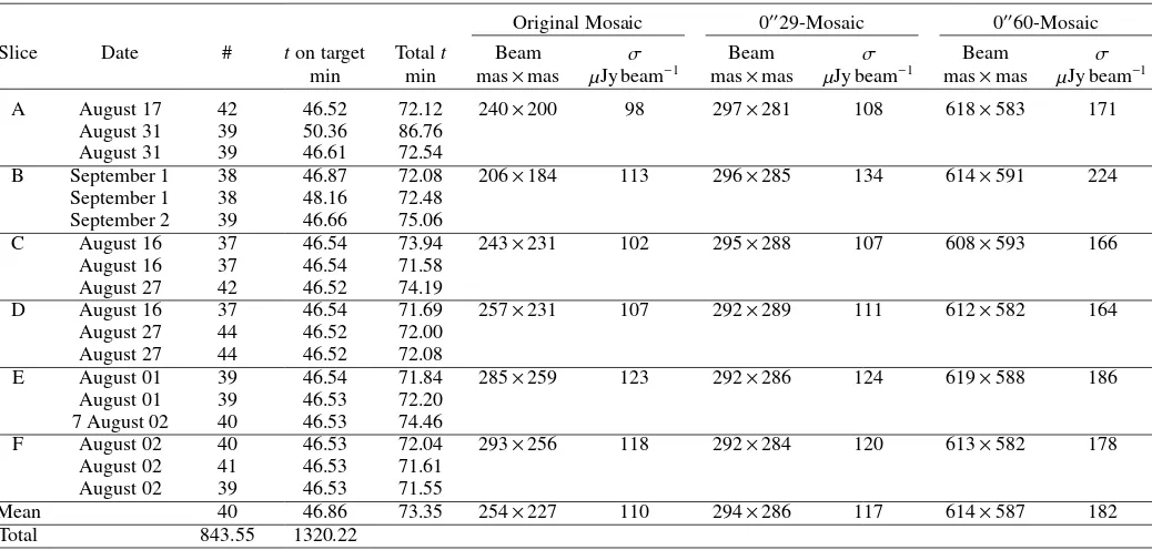
Table 1.Summary of the observations.

Original Mosaic 0′′_{29-Mosaic 0}′′_60-Mosaic

Slice Date # ton target Totalt Beam σ Beam σ Beam σ

min min mas×mas µJy beam−1 _{mas×mas µJy beam}−1 _{mas×mas µJy beam}−1

A August 17 42 46.52 72.12 240×200 98 297×281 108 618×583 171

August 31 39 50.36 86.76

August 31 39 46.61 72.54

B September 1 38 46.87 72.08 206×184 113 296×285 134 614×591 224

September 1 38 48.16 72.48

September 2 39 46.66 75.06

C August 16 37 46.54 73.94 243_×231 102 295_×288 107 608_×593 166

August 16 37 46.54 71.58

August 27 42 46.52 74.19

D August 16 37 46.54 71.69 257×231 107 292×289 111 612×582 164

August 27 44 46.52 72.00

August 27 44 46.52 72.08

E August 01 39 46.54 71.84 285×259 123 292×286 124 619×588 186

August 01 39 46.53 72.20

7 August 02 40 46.53 74.46

F August 02 40 46.53 72.04 293×256 118 292×284 120 613×582 178

August 02 41 46.53 71.61

August 02 39 46.53 71.55

Mean 40 46.86 73.35 254×227 110 294×286 117 614×587 182

Total 843.55 1320.22

Notes.The slice ID, the date, the number of antennae, the time on target, the total time (time on target+calibration time), the resolution and the

1-σnoise of the slice are given.

1000

500

0

500

1000

U [m]

1000

500

0

500

1000

V [m]

Fig. 2.uv-coverage of one of the 846 ALMA pointings constituting this survey. Thisuv-coverage allows us to perform the source detection in the dirty map.

3/Infrared Channel (WFC3/IR) and UVIS channel, along with

the advanced camera for surveys (ACS;Koekemoer et al. 2011.

The area covered by this survey lies in the deep region of the

CANDELS program (central one-third of the field). The 5-σ

detection depth for a point-source reaches a magnitude of 28.16

for the H160 filter (measured within a fixed aperture of 0.17′′

Guo et al. 2013). The CANDELS/Deep program also provides

images in seven other bands: the Y125, J125, B435, V606, i775,

i814 and z850 filters, reaching 5-σ detection depths of 28.45,

28.35, 28.95, 29.35, 28.55, 28.84, and 28.77 mag respectively. The Guo et al.(2013) catalog also includes galaxy magnitudes

from the VLT, taken in theU-band with VIMOS (Nonino et al.

2009), and in theKs-band with ISAAC (Retzlaffet al. 2010) and

HAWK-I (Fontana et al. 2014).

In addition, we used data coming from the FourStar

galaxy evolution survey (ZFOURGE, PI: I. Labbé) on the

6.5 m Magellan Baade telescope. The FourStar instrument

(Persson et al. 2013) observed the CDFS (encompassing the GOODS-South field) through five near-IR medium-bandwidth

filters (J1, J2, J3, Hs,Hl) as well as broad-bandKs. By

com-bination of the FourStar observations in theKs-band and

previ-ous deep and ultra-deep surveys in theK-band, VLT/ISAAC/K

(v2.0) from GOODS (Retzlaffet al. 2010), VLT/HAWK-I/K

from HUGS (Fontana et al. 2014), CFHST/WIRCAM/K from

TENIS (Hsieh et al. 2012) and Magellan/PANIC/K in HUDF

(PI: I. Labbé), a super-deep detection image has been produced. The ZFOURGE catalog reaches a completeness greater than

80% toKs<25.3–25.9 (Straatman et al. 2016).

We used the stellar masses and redshifts from the ZFOURGE catalog, except when spectroscopic redshifts were available.

Stellar masses have been derived fromBruzual & Charlot(2003)

models (Straatman et al. 2016) assuming exponentially

declin-ing star formation histories and a dust attenuation law as

described byCalzetti et al.(2000).

2.4.2. Mid/far-infrared imaging

Data in the mid and far-IR are provided by the infrared

array camera (IRAC; Fazio et al. 2004) at 3.6, 4.5, 5.8, and

8µm,Spitzermultiband imaging photometer (MIPS;Rieke et al.

2004) at 24µm,Herschelphotodetector array camera and

spec-trometer (PACS; Poglitsch et al. 2010) at 70, 100 and 160µm,

andHerschelspectral and photometric imaging receiver (SPIRE;

Griffin et al. 2010) at 250, 350, and 500µm.

The IRAC observations in the GOODS-South field were taken in February 2004 and August 2004 by the GOODS

supplemented by the Spitzerextended deep survey (SEDS; PI:

G. Fazio) at 3.6 and 4.5µm (Ashby et al. 2013) as well as the

Spitzer-cosmic assembly near-infrared deep extragalactic survey

(S-CANDELS;Ashby et al. 2015) and recently by the ultradeep

IRAC imaging at 3.6 and 4.5µm (Labbé et al. 2015).

The flux extraction and deblending in 24µm imaging have

been provided by Magnelli et al. (2009) to reach a depth of

S24 ∼ 30µJy.Herschelimages come from a 206.3 h

GOODS-South observational program (Elbaz et al. 2011) and combined

by Magnelli et al. (2013) with the PACS evolutionary probe

(PEP) observations (Lutz et al. 2011). Because the SPIRE

con-fusion limit is very high, we used the catalog of Wang et al. (in prep.), which is built with a state-of-the-art de-blending method

using optimal prior sources positions from 24µm andHerschel

PACS detections.

2.4.3. Complementary ALMA data

As the GOODS-South field encompasses theHubbleUltra Deep

Field (HUDF), we took advantage of deep 1.3-mm ALMA data of the HUDF. The ALMA image of the full HUDF reaches a σ1.3 mm = 35µJy (Dunlop et al. 2017), over an area of

4.5 arcmin2 _{that was observed using a 45-pointing mosaic at a}

tapered resolution of 0.7′′_{. These observations were taken in two}

separate periods from July to September 2014. In this region, 16

galaxies were detected by Dunlop et al. (2017), three of them

with a high S/N (S/N > 14), the other 13 with lower S/Ns

(3.51<S/N<6.63).

2.4.4. Radio imaging

We also used radio imaging at 5 cm from the Karl G. Jansky Very Large Array (VLA). These data were observed during 2014 March–2015 September for a total of 177 h in the A, B, and C

configurations (PI: W. Rujopakarn). The images have a 0′′_{31 ×}

0′′_{61 synthesized beam and an rms noise at the pointing center}

of 0.32µJy beam−1_{(Rujopakarn et al. 2016). Here, 179 galaxies}

were detected with a significance greater than 3σover an area of

61 arcmin2_{around the HUDF field, with a rms sensitivity better}

than 1µJy beam−1_{. However, this radio survey does not cover the}

entire ALMA area presented in this paper.

2.4.5. X-ray

TheChandradeep field-South (CDF-S) was observed for 7 Msec

between 2014 June and 2016 March. These observations cover

a total area of 484.2 arcmin2_{, offset by just 32}′′ _{from the}

center of our survey, in three X-ray bands: 0.5–7.0 keV, 0.5–

2.0 keV, and 2–7 keV (Luo et al. 2017). The average flux

lim-its over the central region are 1.9_×10−17_{, 6.4×10}−18_{, and}

2.7×10−17_{erg cm}−2_s−1 _{respectively. This survey enhances the}

previous X-ray catalogs in this field, the 4 MsecChandra

expo-sure (Xue et al. 2011) and the 3 Msec XMM-Newton exposure

(Ranalli et al. 2013). We will use this X-ray catalog to identify candidate X-ray active galactic nuclei (AGN) among our ALMA detections.

3. Source detection

The search for faint sources in high-resolution images with moderate source densities faces a major limitation. At the native

resolution (0′′_25×0′′_{23), the untapered ALMA mosaic}

encom-passes almost four million independent beams, where the beam

area is Abeam = π_×FW H M2/(4ln(2)). It results that a search

for sources above a detection threshold of 4-σ would include

as many as 130 spurious sources assuming a Gaussian statistics. Identifying the real sources from such catalog is not possible. In order to increase the detection quality to a level that ensures a purity greater than 80% – in other words, the excess of sources in the original mosaic needs to be five times greater than the

num-ber of detections in the mosaic multiplied by (₋1) – we have

decided to use a tapered image and adapt the detection threshold accordingly.

By reducing the weight of the signal originating from the most peripheral ALMA antennae, the tapering reduces the angular res-olution hence the number of independent beams at the expense of collected light. The lower angular resolution presents the advan-tage of optimizing the sensitivity to point sources – we recall that

0′′_{24 corresponds to a proper size of only 2 kpc atz∼1–3 – and}

therefore will result in an enhancement of the signal-to-noise ratio

(S/N) for the sources larger than the resolution.

We chose to taper the image with a homogeneous and

cir-cular synthesized beam of 0′′_{60 FWHM– corresponding to a}

proper size of 5 kpc at z _∼ 1–3 – having tested various

ker-nels and finding that this beam was optimized for our mosaic, avoiding both a beam degradation and a too heavy loss of sen-sitivity. This tapering reduces by nearly an order of magnitude

the number of spurious sources expected at a 4-σlevel down to

about 19 out of 600 000 independent beams. However, we will check in a second step whether we may have missed in the

pro-cess some compact sources by also analyzing the 0′′_{29 tapered}

map.

We also excluded the edges of the mosaic, where the standard

deviation is larger than 0.30 mJy beam−1 _{in the 0}′′_60-mosaic.

The effective area was thus reduced by 4.9% as compared to the

full mosaic (69.46 arcmin2_{out of 72.83 arcmin}2_).

To identify the galaxies present on the image, we used Blob

-cat(Hales et al. 2012). Blobcatis a source extraction software

using a “flood fill” algorithm to detect and catalog blobs (see

Hales et al. 2012). A blob is defined by two criteria:

– at least one pixel has to be above a threshold (σp)

– all the adjacent surrounding pixels must be above a floodclip

threshold (σf)

whereσp andσf are defined in number ofσ, the local rms of

the mosaic.

A first guess to determine the detection threshold σp is

provided by the examination of the pixel distribution of the

S/N-map. The S/N-map has been created by dividing the 0′′₆₀

tapered map by the noise map. Figure3shows that the S/N-map

follows an almost perfect Gaussian belowS/N=4.2. Above this

threshold, a significant difference can be observed that is

char-acteristic of the excess of positive signal expected in the pres-ence of real sources in the image. However, this histogram alone cannot be used to estimate a number of sources because the pix-els inside one beam are not independent of one another. Hence

although the non-Gaussian behavior appears aroundS/N =4.2

we performed simulations to determine the optimal values ofσp

andσf.

We first conducted positive and negative – on the continuum

map multiplied by (−1) – detection analysis for a range ofσp

andσf values ranging fromσp = 4 to 6 and σf = 2.5 to 4

with intervals of 0.05 and imposing each time σp ≥ σf. The

difference between positive and negative detections for each pair

of (σp,σf) values provides the expected number of real sources.

We then searched for the pair of threshold parameters to find

the best compromise between(i)providing the maximum

5.0

2.5 0.0

2.5

5.0

7.5 10.0

SNR

10

10

10

10

10

10

10

N

-0.90 -0.45 0.00 0.45 0.90 1.35 1.80

S

[mJy.beam

]

Fig. 3.Histogram of pixels of the S/N map, where pixels with noise

>0.3 mJy beam−1 _{have been removed. The red dashed line is the best}

Gaussian fit. The green dashed line is indicative and shows where the pixel brightness distribution moves away from the Gaussian fit. This is also the 4.2σlevel corresponding to a peak flux of 0.76 mJy for a typical noise per beam of 0.18 mJy. The solid black line corresponds to our peak threshold of 4.8σ(0.86 mJy).

sources. The later purity criterion,pc, is defined as:

pc=

Np−Nn

Np (1)

whereNpandNnare the numbers of positive and negative

detec-tions respectively. To ensure a purity of 80% as discussed above,

we enforced pc ≥ 0.8. This led to σp = 4.8σ when fixing

the value of σf = 2.7σ (see Fig. 4-left). Below σp = 4.8σ,

the purity criterion rapidly drops below 80% whereas above this

value it only mildly rises. Fixingσp =4.8σ, the purity remains

roughly constant at_∼80_±5% when varyingσf. We did see an

increase in the difference between the number of positive and

negative detections with increasingσf. However, the size of the

sources above σf = 2.7σ drops below the 0′′60 FWHMand

tends to become pixel-like, hence non physical. This is because

an increase of σf results in a reduction of the number of

pix-els above the floodclip threshold (σf) that will be associated

with a given source. This parameter can be seen as a percola-tion criterion that sets the size of the sources in a number of

pix-els. Reversely reducing σf below 2.7σresults in adding more

noise than signal and a reduction in the number of detections.

We therefore decided to setσf to 2.7σ.

While we did not wish to impose a criterion on the existence of optical counterparts to define our ALMA catalog, we found

that high values ofσf not only generate the problem discussed

above, but also generate a rapid drop of the fraction of ALMA

detections with an HST counterpart in theGuo et al.(2013)

cat-alog, pHST = NHST/Np.NHSTis the number of ALMA sources

with an HST counterpart within 0′′_{60 (corresponding to the size}

of the beam). The fraction falls rapidly from around ∼80% to

∼60%, which we interpreted as being due to a rise of the

propor-tion of spurious sources, since the faintest optical sources, for example, detected by HST-WFC3, are not necessarily associated

with the faintest ALMA sources due to the negativeK-correction

at 1.1 mm. This rapid drop can be seen in the dashed green and

dotted pink lines of Fig.4-right. This confirms that the sources

that are added to our catalog with a floodclip threshold greater

than 2.7σare most probably spurious. Similarly, we can see in

Fig.4-left that increasing the number of ALMA detections to

fainter flux densities by reducingσpbelow 4.8σleads to a rapid

drop of the fraction of ALMA detections with an HST counter-part. Again there is no well-established physical reason to expect the number of ALMA detections with an optical counterpart to

decrease with decreasing S/N ratio in the ALMA catalog.

As a result, we decided to setσp =4.8σandσf =2.7σto

produce our catalog of ALMA detections. We note that we only discussed the existence of HST counterparts as a complementary test on the definition of the detection thresholds but our approach is not set to limit in any way our ALMA detections to galaxies with HST counterparts.

Indeed, evidence for the existence of ALMA detections with no HST-WFC3 counterparts already exist in the literature.

Wang et al.(2016) identifiedH-dropouts galaxies, that is

galax-ies detected above theH-band withSpitzer-IRAC at 4.5µm but

undetected in the H-band and in the optical. The median flux

density of these galaxies isF870µm ≃ 1.6 mJy (Wang et al., in

prep.). By scaling this median value to our wavelength of 1.1 mm

(the details of this computation are given in Sect.5.4), we obtain

a flux density of 0.9 mJy, close to the typical flux of our

detec-tions (median flux∼1 mJy, see Table3).

4. Catalog

4.1. Creation of the catalog

Using the optimal parameters of σp = 4.8σ andσf = 2.7σ

described in Sect.3, we obtained a total of 20 detections down to

a flux density limit ofS1.1 mm≈880µJy that constitute our main

catalog. These detections can be seen ranked by their S/N in

Fig.1. The comparison of negative and positive detections

sug-gests the presence of 4_±2 (assuming a Poissonian uncertainty

on the difference between the number of positive and negative

detections) spurious sources in this sample.

In the following, we assume that the galaxies detected in the

0′′_{60-mosaic are point-like. This hypothesis will later be}

dis-cussed and justified in Sect.4.5. In order to check the robustness

of our flux density measurements, we compared different flux

extraction methods and softwares: PyBDSM(Mohan & Rafferty

2015);Galfit(Peng et al. 2010);Blobcat(Hales et al. 2012).

The peak flux value determined byBlobcatrefers to the peak

of the surface brightness corrected for peak bias (seeHales et al.

2012). The different results were consistent, with a median ratio

of FBlobcat

peak /F

PyBDSM

peak = 1.04 ±0.20 and FBlobcatpeak /FGalfitPSF =

0.93_±0.20. The fluxes measured using psf-fitting (Galfit) and

peak flux measurement (Blobcat) for each galaxy are listed in

Table3. We also ran CASAfitskyand a simple aperture

pho-tometry corrected for the ALMA PSF and also found consistent

results. The psf-fitting withGalfitwas performed inside a box

of 5×5′′_{centered on the source.}

The main characteristics of these detections (redshift, flux,

S/N, stellar mass, counterpart) are given in Table 3. We used

redshifts and stellar masses from the ZFOURGE catalog (see

Sect.2.4.1).

We compared the presence of galaxies between the 0′′

60-mosaic and the 0′′_{29-mosaic. Of the 20 detections found in the}

0′′_{60 map, 14 of them are also detected in the 0}′′_{29 map. The}

4.00 4.25 4.50 4.75 5.00 5.25 5.50 5.75 6.00

p ( f = 2.7)

100

101

102

N

Positive Negative

0.0 0.2 0.4 0.6 0.8 1.0

pc

,

pHS

T

,

pZFOUR

GE

2.50 2.75 3.00 3.25 3.50 3.75 4.00

f ( p = 4.8)

0 10 20 30 40

N

Positive Negative

0.0 0.2 0.4 0.6 0.8 1.0

pc

,

pHS

T

,

pZF

O

U

R

GE

Fig. 4.Cumulative number of positive (red histogram) and negative (blue histogram) detections as a function of theσp(at a fixedσf,left panel) andσf (at a fixedσp,right panel) in units ofσ. Solid black line represents the purity criterionpcdefine by Eq. (1), green dashed-line represents

the percentage of positive detection with HST-WFC3 counterpart pHSTand magenta dashed-line represents the percentage of positive detection

with ZFOURGE counterpartpZFOURGE. Gray dashed-lines show the thresholdsσp=4.8σandσf =2.7σand the 80% purity limit.

a more compact source is more likely to be missed in the maps with larger tapered sizes and reduced point source sensitivity.

A first method to identify potential false detections was to compare our results with a deeper survey overlapping with our area of the sky. We compared the positions of our catalog sources

with the positions of sources found byDunlop et al.(2017) in

the HUDF. This 1.3-mm image is deeper than our survey and

reaches aσ _≃35µJy (corresponding toσ=52µJy at 1.1 mm)

but overlaps with only∼6.5% of our survey area. The final

sam-ple of Dunlop et al.(2017) was compiled by selecting sources

withS1.3 >120µJy to avoid including spurious sources due to

the large number of beams in the mosaics and due to their choice of including only ALMA detections with optical counterparts seen with HST.

With our flux density limit of S1.1 mm ≈ 880µJy any

non-spurious detection should be associated with a source seen at 1.3 mm in the HUDF 1.3 mm survey, the impact of the

wave-length difference being much smaller than this ratio. We detected

three galaxies that were also detected byDunlop et al.(2017),

UDF1, UDF2 and UDF3, all of which haveS1.3 mm >0.8 mJy.

The other galaxies detected byDunlop et al.(2017) have a flux

density at 1.3 mm lower than 320µJy, which makes them

unde-tectable with our sensitivity.

We note however that we did not impose as a strict criterion the existence of an optical counterpart to our detections, whereas

Dunlop et al.(2017) did. Hence if we had detected a source with no optical counterpart within the HUDF, this source may not

be included in theDunlop et al.(2017) catalog. However, as we

will see, the projected density of such sources is small and none of our candidate optically dark sources fall within the limited area of the HUDF. We also note that the presence of an

HST-WFC3 source within a radius of 0′′_{6 does not necessarily imply}

that is the correct counterpart. As we will discuss in detail in

Sect.4.4, due to the depth of the HST-WFC3 observations and

the large number of galaxies listed in the CANDELS catalog, a match between the HST and ALMA positions may be possible

by chance alignment alone (see Sect.4.4).

4.2. Supplementary catalog

After the completion of the main catalog, three sources that did not satisfy the criteria of the main catalog presented strong

evidence of being robust detections. We therefore enlarged our catalog, in order to incorporate these sources into a supplemen-tary catalog.

These three sources are each detected using a combination

ofσpandσfgiving a purity factor greater than 80%, whilst also

ensuring the existence of an HST counterpart.

The galaxy AGS21 has anS/N = 5.83 in the 0′′29 tapered

map, but is not detected in the 0′′_{60 tapered map. The}

non-detection of this source is most likely caused by its size. Due to

its dilution in the 0′′_{60-mosaic, a very compact galaxy detected}

at 5σin the 0′′_{29-mosaic map could be below the detection limit}

in the 0′′_{60-mosaic. The ratio of the mean rms of the two tapered}

maps is 1.56, meaning that for a point source of certain flux, a

5.83σmeasurement in the 0′′29-mosaic becomes 3.74σ in the

0′′_60-map.

The galaxy AGS22 has been detected with an S/N = 4.9

in the 0′′_{60 tapered map (σp = 4.9 andσf = 3.1). With σp}

andσf values more stringent than the thresholds chosen for the

main catalog, it may seem paradoxical that this source does not

appear in the main catalog. With a floodclip criterion of 2.7σ,

this source would have an S/N just below 4.8, excluding it from

the main catalog. This source is associated with a faint galaxy

that has been detected by HST-WFC3 (IDCANDELS =28 952) at

1.6µm (6.6σ) at a position close to the ALMA detection (0′′_28).

Significant flux has also been measured at 1.25µm (3.6σ) for

this galaxy. In all of the other filters, the flux measurement is

not significant (<3σ). Due to this lack of information, it has not

been possible to compute its redshift. AGS22 is not detected in

the 0′′_{29-mosaic map withpc>0.8. The optical counterpart of}

this source has a lowH-band magnitude (26.8_±0.2 AB), which

corresponds to a range for which theGuo et al.(2013) catalog

is no longer complete. This is the only galaxy (except the three galaxies most likely to be spurious: AGS14, AGS16 and AGS19) that has not been detected by IRAC (which could possibly be explained by a low stellar mass). The probability of the ALMA

detection being spurious, within the association radius 0′′_{6 of a}

H-band source of this magnitude or brighter, is 5.5%. For these

reasons, we did not consider it as spurious.

The galaxy AGS23 was detected in the 0′′_{60 map just}

below our threshold at 4.8σ, with a combination σp = 4.6

andσf = 2.9 giving a purity criterion greater than 0.9. This

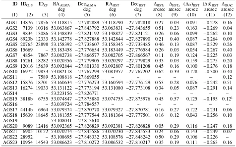
Table 2.Details of the positional differences between ALMA and HST-WFC3 for our catalog of galaxies identified in the 1.1 mm-continuum map.

ID IDCLS IDZF RAALMA DecALMA RAHST DecHST ∆HST1 ∆HST2 (∆α)HST (∆δ)HST ∆IRAC

deg deg deg deg arcsec arcsec arcsec arcsec arcsec

(1) (2) (3) (4) (5) (6) (7) (8) (9) (10) (11) (12)

AGS1 14876 17856 53.118815 ₋27.782889 53.118790 ₋27.782818 0.27 0.03 0.091 ₋0.278 0.16

AGS2 7139 10316 53.063867 −27.843792 53.063831 −27.843655 0.51 0.23 0.163 −0.269 0.04

AGS3 9834 13086 53.148839 ₋27.821192 53.148827 ₋27.821121 0.26 0.06 0.099 ₋0.262 0.10

AGS4 8923b 12333 53.142778 −27.827888 53.142844 −27.827890 0.21 0.40 0.087 −0.264 0.09

AGS5 20765 23898 53.158392 ₋27.733607 53.158345 ₋27.733485 0.46 0.13 0.087 ₋0.329 0.26

AGS6 15669 – 53.183458 −27.776654 53.183449 −27.776584 0.26 0.03 0.054 −0.267 0.40

AGS7 4854 7867 53.082738 ₋27.866577 53.082705 ₋27.866567 0.11 0.19 0.124 ₋0.225 0.03

AGS8 15261 18282 53.020356 ₋27.779905 53.020297 ₋27.779829 0.33 0.03 0.159 ₋0.275 0.20

AGS9 12016 15639 53.092844 −27.801330 53.092807 −27.801208 0.45 0.16 0.100 −0.276 0.18

AGS10 16972 19833 53.082118 ₋27.767299 53.081957 ₋27.767202 0.62 0.39 0.128 ₋0.300 0.40

AGS11 – 7589 53.108818 −27.869055 – – – – – – 0.12

AGS12 15876 18701 53.160634 ₋27.776273 53.160594 ₋27.776129 0.53 0.28 0.076 ₋0.242 0.51

AGS13 16274 19033 53.131122 −27.773194 53.131080 −27.773108 0.34 0.05 0.087 −0.291 0.14

AGS14 – – 53.223156 ₋27.826771 – – – – – – –

AGS15 3818b 6755 53.074847 ₋27.875880 53.074755 ₋27.875976 0.45 0.57 0.125 ₋0.195 0.121

AGS16 – – 53.039724 −27.784557 – – – – – – –

AGS17 4414b 6964 53.079374 ₋27.870770 53.079327 ₋27.870781 0.16 0.27 0.122 ₋0.231 0.06

AGS18 15639 18645 53.181355 −27.777544 53.181364 −27.777501 0.16 0.12 0.043 −0.256 0.10

AGS19 – – 53.108041 ₋27.813610 – – – – – – –

AGS20 9089 12416 53.092365 −27.826829 53.092381 −27.826828 0.05 0.29 0.116 −0.247 0.18

AGS21 6905 10152 53.070274 −27.845586 53.070230 −27.845533 0.24 0.06 0.143 −0.249 0.07

AGS22 28952 – 53.108695 ₋27.848332 53.108576 ₋27.848242 0.50 0.29 0.106 ₋0.226 –

AGS23 10954 14543 53.086623 −27.810272 53.086532 −27.810217 0.35 0.19 0.111 −0.263 0.16

Notes.Columns: (1) Source ID; (2),(3) IDs of the HST-WFC3 (from the CANDELS catalog) and ZFOURGE counterparts of these detections (the cross correlations between ALMA and HST-WFC3 and between ALMA and ZFOURGE are discussed in Sect.4.4). b indicates HST-WFC3 galaxies located in a radius of 0′′_{6 around the ALMA detection, although strong evidence presented in Sect.7suggests they are not the}

opti-cal counterparts of our detections; (4), (5) RA and Dec of the sources in the ALMA image (J2000); (6), (7) positions of HST-WFC3 H-band counterparts when applicable fromGuo et al.(2013), (8), (9) distances between the ALMA and HST source positions before (∆HST1) and after

(∆HST2) applying the offset correction derived from the comparison with Pan-STARRS andGaia; (10), (11) offset to be applied to the HST source

positions, which includes both the global systematic offset and the local offset; (12) distance from the closest IRAC galaxy.(1)For AGS15 we used

the distance given in the ZFOURGE catalog (see Sect.7).

for these two reasons that we include this galaxy in the

sup-plementary catalog. The photometric redshift (z = 2.36) and

stellar mass (1011.26_M

⊙) both reinforce the plausibility of this

detection.

4.3. Astrometric correction

The comparison of our ALMA detections with HST (Sect.4.1)

in the previous section was carried out after correcting for an

astrometric offset, which we outline here. In order to perform

the most rigorous counterpart identification and take advan-tage of the accuracy of ALMA, we carefully investigated the astrometry of our images. Before correction, the galaxy positions

viewed by HST were systematically offset from the ALMA

posi-tions. This offset has already been identified in previous studies

(e.g.,Maiolino et al. 2015;Rujopakarn et al. 2016;Dunlop et al.

2017).

In order to quantify this effect, we compared the HST source

positions with detections from the Panoramic Survey Telescope and Rapid Response System (Pan-STARRS). This survey has the double advantage to cover a large portion of the sky, notably the GOODS-South field, and to observe the sky at a wavelength similar to HST-WFC3. We used the Pan-STARRS DR1 catalog

provided by Flewelling et al. (2016) and also included the

corresponding regions issued from the Gaia DR1

(Gaia Collaboration 2016).

Cross-matching was done within a radius of 0′′_{5. In order}

to minimize the number of false identifications, we subtracted

the median offset between the two catalogs from theGuo et al.

(2013) catalog positions, after the first round of matching. We

iterated this process three times. In this way, 629 pairs were found over the GOODS-South field.

To correct for the median offset between the HST and ALMA

images, the HST image coordinates needed to be corrected by

−96±113 mas in right ascension,α, and 261_±125 mas in

dec-lination, δ, where the uncertainties correspond to the standard

deviation of the 629 offset measurements. This offset is

con-sistent with that found by Rujopakarn et al. (2016) of ∆α =

−80±110 mas and∆δ= 260_±130 mas. The latter offsets were

calculated by comparing the HST source positions with 2MASS and VLA positions. In all cases, it is the HST image that presents

an offset, whereas ALMA, Pan-STARRS, Gaia, 2MASS and

VLA are all in agreement. We therefore deduced that it is the astrometric solution used to build the HST mosaic that

intro-duced this offset. As discussed in Dickinson et al. (in prep.),

the process of building the HST mosaic also introduced less

significant local offsets, that can be considered equivalent to a

Table 3.Details of the final sample of sources detected in the ALMA GOODS-South continuum map, from the primary catalog in the main part of the table and from the supplementary catalog below the solid line (see Sects.4.1and4.2).

ID z S/N SBlobcat

peak fdeboost SGalfitPSF log10 M⋆ 0′′60 0′′29 S6 GHz LX/1042 IDsub(mm)

mJy mJy M_⊙ µJy erg s−1

(1) (2) (3) (4) (5) (6) (7) (8) (9) (10) (11) (12)

AGS1 2.309 11.26 1.90±0.20 1.03 1.99±0.15 11.05 1 1 18.38±0.71 1.93 GS6, ASA1

AGS2 2.918 10.47 1.99_±0.22 1.03 2.13_±0.15 10.90 1 1 – 51.31

AGS3 2.582 9.68 1.84±0.21 1.03 2.19±0.15 11.33 1 1 19.84±0.93 34.54 GS5, ASA2

AGS4 4.32 9.66 1.72_±0.20 1.03 1.69_±0.18 11.45 1 1 8.64_±0.77 10.39

AGS5 3.46 8.95 1.56_±0.19 1.03 1.40_±0.18 11.13 1 1 14.32_±1.05 37.40

AGS6 3.00 7.63 1.27±0.18 1.05 1.26±0.16 10.93 1 1 9.02±0.57 83.30 UDF1, ASA3

AGS7 3.29 7.26 1.15_±0.17 1.05 1.20_±0.13 11.43 1 1 – 24.00

AGS8 1.95 7.10 1.43±0.22 1.05 1.98±0.20 11.53 1 1 – 3.46 LESS18

AGS9 3.847 6.19 1.25_±0.21 1.05 1.39_±0.17 10.70 1 1 14.65_±1.12 –

AGS10 2.41 6.10 0.88±0.15 1.06 1.04±0.13 11.32 1 1 – 2.80

AGS11 4.82 5.71 1.34_±0.25 1.08 1.58_±0.22 10.55 1 1 – –

AGS12 2.543 5.42 0.93_±0.18 1.10 1.13_±0.15 10.72 1 1 12.65_±0.55 4.53 UDF3, C1, ASA8

AGS13 2.225 5.41 0.78±0.15 1.10 0.47±0.14 11.40 1 0 22.52±0.81 13.88 ASA12

AGS14* – 5.30 0.86_±0.17 1.10 1.17_±0.15 – 1 0 – –

AGS15 – 5.22 0.80±0.16 1.11 0.64±0.15 – 1 1 – – LESS34

AGS16* – 5.05 0.82_±0.17 1.12 0.99_±0.17 – 1 0 – –

AGS17 – 5.01 0.93±0.19† 1.14 1.37±0.18 – 1 0 – – LESS10

AGS18 2.794 4.93 0.85_±0.18_† 1.15 0.79_±0.15 11.01 1 0 6.21_±0.57 – UDF2, ASA6

AGS19* – 4.83 0.69±0.15 1.16 0.72±0.13 – 1 0 – –

AGS20 2.73 4.81 1.11_±0.24 1.16 1.18_±0.23 10.76 1 1 12.79_±1.40 4.02

AGS21 3.76 5.83 0.64_±0.11 1.07 0.88_±0.19 10.63 0 1 – 19.68

AGS22 – 4.90 1.05±0.22 1.15 1.26±0.22 – 1 0 – –

AGS23 2.36 4.68 0.98_±0.21 1.19 1.05_±0.20 11.26 1 0 – –

Notes.Columns: (1) IDs of the sources as shown in Fig.1. The sources are sorted by S/N. * indicates galaxies that are most likely spurious (not

detected at any other wavelength); (2) redshifts from the ZFOURGE catalog. Spectroscopic redshifts are shown with three decimal places. As AGS6 is not listed in the ZFOURGE catalog, we used the redshift computed byDunlop et al.(2017); (3) S/N of the detections in the 0′′_{60 mosaic}

(except for AGS21). This S/N is computed using the flux fromBlobcatand is corrected for peak bias; (4) peak fluxes measured usingBlobcatin

the 0′′_{60-mosaic image before de-boosting correction; (5) deboosting factor; (6) fluxes measured by PSF-fitting withGalfitin the 0}′′_60-mosaic

image before de-boosting correction; (7) stellar masses from the ZFOURGE catalog; (8), (9) flags for detection byBlobcatin the 0′′_60-mosaic

and 0′′_{29-mosaic images, where at least one combination ofσ}

p andσf gives a purity factor (Eq. (1)) greater than 80%; (10) flux for detection greater than 3σby VLA (5 cm). Some of these sources are visible in the VLA image but not detected with a threshold>3σ. AGS8 and AGS16 are not in the field of the VLA survey; (11) absorption-corrected intrinsic 0.5–7.0 keV luminosities. The X-ray luminosities have been corrected to account for the redshift difference between the redshifts provided in the catalog ofLuo et al.(2017) and those used in the present table, when

necessary. For this correction we used Eq. (1) fromAlexander et al.(2003), and assuming a photon index ofΓ =2; (12) corresponding IDs for

detections of the sources in previous (sub)millimeter ancillary data. UDF is forHubbleUltra Deep Field survey (Dunlop et al. 2017) at 1.3 mm, C indicates the ALMA Spectroscopic Survey in theHubbleUltra Deep Field (ASPECS) at 1.2 mm (Aravena et al. 2016), LESS indicates data at 870µm presented inHodge et al.(2013), GS indicates data at 870µm presented inElbaz et al.(2018), ASA indicates the ALMA 26 arcmin2 Survey of GOODS-S at One-millimeter (ASAGAO). We also note the pointed observations of AGS1 presented inBarro et al.(2017), and those of AGS13 byTalia et al.(2018). For the two sources marked by a†, the hypothesis a of a point-like source is no longer valid. We therefore apply

correction factors of 2.3 and 1.7 to the peak flux values of AGS17 and AGS18 respectively, to take into account the extended flux emission of these sources.

the periphery of GOODS-South than in the center, and close

to zero in the HUDF field. The local offsets can be considered

as a distortion effect. The offsets listed in Table2 include both

effects, the global and local offsets. The separation between HST

and ALMA detections before and after offset correction, and

the individual offsets applied for each of the galaxies are

indi-cated in Table2and can be visualized in Fig.5. We applied the

same offset corrections to the galaxies listed in the ZFOURGE

catalog.

This accurate subtraction of the global systematic offset, as

well as the local offset, does not however guarantee a perfect

overlap between ALMA and HST emission. The location of the

dust emission may not align perfectly with the starlight from a

galaxy, due to the difference in ALMA and HST resolutions, as

well as the physical offsets between dust and stellar emission that

may exist. In Fig.6, we show the ALMA contours (4–10σ)

over-laid on the F160W HST-WFC3 images after astrometric correc-tion. In some cases (AGS1, AGS3, AGS6, AGS13, AGS21 for example), the position of the dust radiation matches that of the stellar emission; in other cases, (AGS4, AGS17 for example), a displacement appears between both two wavelengths. Finally, in some cases (AGS11, AGS14, AGS16, and AGS19) there are no optical counterparts. We will discuss the possible explanations

0.6 0.4 0.2 0.0 0.2 0.4 0.6

["] 0.6

0.4 0.2 0.0 0.2 0.4 0.6

[

"]

Before correction After correction

Fig. 5.Positional offset (RAHST–RAALMA, DecHST–DecALMA) between

HST and ALMA before (red crosses) and after (blue crosses) the cor-rection of both a global systematic offset and a local offset. The black

dashed circle corresponds to the cross-matching limit radius of 0′′_{6. The}

gray dashed circles show a positional offset of 0′′_{2 and 0}′′_{4 respectively.}

The magenta lines indicate the HST galaxies previously falsely associ-ated with ALMA detections.

4.4. Identification of counterparts

We searched for optical counterparts in the

CANDELS/GOODS-South catalog, within a radius of 0′′₆

from the millimeter position after applying the astrometric

corrections to the source positions described in Sect. 4.3. The

radius of the cross-matching has been chosen to correspond to

the synthesized beam (0′′_{60) of the tapered ALMA map used}

for galaxy detection. Following Condon (1997), the maximal

positional accuracy of the detection in the 1.1 mm map is given

byθbeam/(2×S/N). In the 0′′60-mosaic, the positional accuracy

therefore ranges between 26.5 mas and 62.5 mas for our range

of S/N (4.8–11.3), corresponding to physical sizes between 200

and 480 pc atz=3.

Despite the high angular resolution of ALMA, the chance of an ALMA-HST coincidence is not negligible, because of

the large projected source density of the CANDELS/

GOODS-South catalog. Figure 7 shows a Monte Carlo simulation

per-formed to estimate this probability. We separate here the deeper

HubbleUltra Deep Field (blue histogram) from the rest of the

CANDELS-deep area (orange histogram). We randomly defined a position within GOODS-South and then measured the dis-tance to its closest HST neighbor using the source positions

listed inGuo et al.(2013). We repeated this procedure 100 000

times inside and outside the HUDF. The probability for a posi-tion randomly selected in the GOODS-South field to fall within 0.6 arcsec of an HST source is 9.2% outside the HUDF, and 15.8% inside the HUDF. We repeated this exercise to test the

presence of an IRAC counterpart with the Ashby et al.(2015)

catalog (green histogram). The probability to randomly fall on an IRAC source is only 2.1%.

With the detection threshold determined in Sect. 3, 80%

of the millimeter galaxies detected have an HST-WFC3 coun-terpart, and four galaxies remain without an optical

counter-part. We cross-matched our detections with the ZFOURGE catalog.

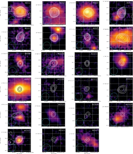
Figure 8 shows 3′′_5×3′′_{5 postage stamps of the}

ALMA-detected galaxies, overlaid with the positions of galaxies

from the CANDELS/GOODS-South catalog (magenta double

crosses), ZFOURGE catalog (white circles) or both catalogs

(sources with an angular separation lower than 0′′_{4, blue}

cir-cles). These are all shown after astrometric correction. Based on the ZFOURGE catalog, we found optical counterparts for one galaxy that did not have an HST counterpart: AGS11, a photo-metric redshift has been computed in the ZFOURGE catalog for this galaxy.

The redshifts of AGS4 and AGS17 as given in the

CANDELS catalog are unexpectedly low (z=0.24 andz=0.03,

respectively), but the redshifts for these galaxies given in the

ZFOURGE catalog (z = 3.76 and z = 1.85, respectively)

are more compatible with the expected redshifts for galaxies detected with ALMA. These galaxies, missed by the HST or incorrectly listed as local galaxies are particularly interesting

galaxies (see Sect.7). AGS6 is not listed in the ZFOURGE

cat-alog, most likely because it is close (<0′′_{7) to another bright}

galaxy (IDCANDELS = 15 768). These galaxies are blended in

the ZFOURGE ground-based Ks-band images. AGS6 has

pre-viously been detected at 1.3 mm in the HUDF, so we adopt the

redshift and stellar mass found byDunlop et al.(2017). The

con-sensus CANDELS zphot fromSantini et al.(2015) isz =3.06

(95% confidence: 2.92<z<3.40), consistent with the value in

Dunlop et al.(2017).

4.5. Galaxy sizes

Correctly estimating the size of a source is an essential ingre-dient for measuring its flux. As a first step, it is imperative to know if the detections are resolved or unresolved. In this section, we discuss our considerations regarding the sizes of our galax-ies. The low number of galaxies with measured ALMA sizes in

the literature makes it difficult to constrain the size distribution

of dust emission in galaxies. Recent studies (e.g., Barro et al.

2016; Rujopakarn et al. 2016; Elbaz et al. 2018; Ikarashi et al. 2017;Fujimoto et al. 2017) with sufficient resolution to measure

ALMA sizes of galaxies suggest that dust emission takes place within compact regions of the galaxy.

Two of our galaxies (AGS1 and AGS3) have been observed in individual pointings (ALMA Cycle 1; P.I. R. Leiton,

pre-sented inElbaz et al. 2018) at 870µm with a long integration

time (40–50 min on source). These deeper observations give more information on the nature of the galaxies, in particular on

their morphology. Due to their high S/N (_∼100) the sizes of the

dust emission could be measured accurately:R1/2maj =120±4

and 139±6 mas for AGS1 and AGS3 respectively, revealing

extremely compact star-forming regions corresponding to

cir-cularized effective radii of _∼1 kpc at redshift z _∼ 2. The

Ser-sic indices are 1.27_±0.22 and 1.15_±0.22 for AGS1 and AGS3

respectively: the dusty star-forming regions therefore seem to be

disk-like. Based on their sizes, their stellar masses (>1011M_⊙),

their SFRs (>103M_⊙yr−1_{) and their redshifts (z∼2), these very}

compact galaxies are ideal candidate progenitors of compact

quiescent galaxies at z _∼ 2 (Barro et al. 2013; Williams et al.

2014; van der Wel et al. 2014; Kocevski et al. 2017, see also

Elbaz et al. 2018).

Size measurements of galaxies at (sub)millimeter

wave-lengths have previously been made as part of several different

studies. Ikarashi et al. (2015) measured sizes for 13

3h32m28.45s 28.50s 28.55s 59.0" 58.5" -27°46'58.0" Dec (J2000) AGS1 3h32m15.30s 15.35s 15.40s 38.5" 38.0" 37.5" -27°50'37.0" AGS2 3h32m35.70s 35.75s 17.0" 16.5" 16.0" -27°49'15.5" AGS3 3h32m34.25s 34.30s 41.0" 40.5" 40.0" -27°49'39.5" _AGS4 3h32m37.95s 38.00s 38.05s 01.5" 01.0" -27°44'00.5" Dec (J2000) AGS5 3h32m44.00s 44.05s 44.10s 36.5" 36.0" -27°46'35.5" AGS6 3h32m19.80s 19.85s 19.90s 00.5" 52'00.0" 59.5" -27°51'59.0" AGS7 3h32m04.85s 04.90s 04.95s 48.5" 48.0" 47.5" -27°46'47.0" AGS8 3h32m22.25s 22.30s 22.35s 05.5" 05.0" 04.5" -27°48'04.0" Dec (J2000) AGS9 3h32m19.65s 19.70s 19.75s 03.0" 02.5" 02.0" -27°46'01.5" AGS10 3h32m26.05s 26.10s 26.15s 09.5" 09.0" 08.5" -27°52'08.0" AGS11 3h32m38.50s 38.55s 38.60s 35.5" 35.0" 34.5" -27°46'34.0" AGS12 3h32m31.45s 31.50s 24.0" 23.5" -27°46'23.0" Dec (J2000) AGS13 3h32m53.50s 53.55s 53.60s 37.0" 36.5" 36.0" -27°49'35.5" _AGS14 3h32m17.90s 17.95s 18.00s 34.0" 33.5" 33.0" -27°52'32.5" AGS15 3h32m09.50s 09.55s 09.60s 05.0" 04.5" -27°47'04.0" AGS16 3h32m19.00s 19.05s 19.10s 15.5" 15.0" 14.5" -27°52'14.0" Dec (J2000) AGS17 3h32m43.50s 43.55s 40.0" 39.5" 39.0" -27°46'38.5" AGS18 3h32m25.90s 25.95s 26.00s 49.5" 49.0" -27°48'48.5" AGS19 3h32m22.15s 22.20s 37.5" 37.0" 36.5" -27°49'36.0" AGS20 3h32m16.80s 16.85s

16.90s_{RA (J2000)}

45.0" 44.5" 44.0" -27°50'43.5" Dec (J2000) AGS21 3h32m26.05s 26.10s

26.15s _{RA (J2000)} 54.5" 54.0" -27°50'53.5" AGS22 3h32m20.75s 20.80s

20.85s _{RA (J2000)} 37.5"

37.0" -27°48'36.5"

AGS23

Fig. 6.Postage stamps of 1.8×1.8 arcsec. ALMA contours (4, 4.5 then 5–10-σwith a step of 1-σ) at 1.1 mm (white lines) are overlaid on F160W HST/WFC3 images. The images are centered on the ALMA detections. The shape of the synthesized beam is given in the bottom left corner.

Astrometry corrections described in Sect.4.3have been applied to the HST images. In some cases (AGS1, AGS3, AGS6, AGS13, AGS21 for example), the position of the dust radiation matches that of the stellar emission; in other cases, (AGS4, AGS17 for example), a displacement appears between both two wavelengths. Finally, in some cases (AGS11, AGS14, AGS16, and AGS19) there are no optical counterparts. We will discuss the possible explanations for this in Sect.7.

0′′_{38 with a median of 0}′′₂₀+0′′₀₃

−0′′05 at 1.1 mm. Simpson et al.

(2015a) derived a median intrinsic angular size of FW H M =

0′′_30±0′′_{04 for their 23 detections with a S/N > 10 in the}

Ultra Deep Survey (UDS) for a resolution of 0′′_{3 at 870µm.}

Tadaki et al.(2017) found a median FWHM of 0′′_{11±0.02 for}

12 sources in a 0′′_{2-resolution survey at 870µm. Barro et al.}

(2016) use a high spatial resolution (FW H M _∼ 0′′_{14) to}

measure a median Gaussian FWHM of 0′′_{12 at 870µm, with}

an average Sersic index of 1.28. For Hodge et al. (2016), the

median major axis size of the Gaussian fit is FW H M =

0′′_{42 ± 0}′′_{04 with a median axis ratio b/a = 0.53±0.03}

for 16 luminous ALESS SMGs, using high-resolution (_∼0′′₁₆₎

data at 870µm. Rujopakarn et al. (2016) found a median

cir-cular FWHM at 1.3 mm of 0′′_{46 from the ALMA image of}

the HUDF (Dunlop et al. 2017). González-López et al. (2017)