Double Chain Ladder

City, University of London Institutional Repository

Citation

: Martinez-Miranda, M. D., Nielsen, J. P. and Verrall, R. J. (2012). Double Chain

This is the unspecified version of the paper.

This version of the publication may differ from the final published

version.

Permanent repository link:

Link to published version

:

Copyright and reuse:

City Research Online aims to make research

outputs of City, University of London available to a wider audience.

Copyright and Moral Rights remain with the author(s) and/or copyright

holders. URLs from City Research Online may be freely distributed and

linked to.

City Research Online: http://openaccess.city.ac.uk/ [email protected]

Double Chain Ladder

Mar´ıa Dolores Mart´ınez Miranda

University of Granada, Spain [email protected]

Jens Perch Nielsen

Cass Business School, City University, London, U.K. [email protected]

Richard Verrall

Cass Business School, City University, London, U.K. [email protected]

August 4, 2011

Abstract

By adding the information of reported count data to a classical triangle of reserving data, we derive a suprisingly simple method for forecasting IBNR and RBNS claims. A simple relationship between development factors allows to involve and then estimate the reporting and payment delay. Bootstrap methods provide prediction errors and make possible the inference about IBNR and RBNS claims, separately.

Keywords: Bootstrapping; Chain Ladder; Claims Reserves; Reserve Risk

1

Introduction

that any extensions or alterations also have an ad hoc flavour, including the way in which tail factors are produced; the way in which data is adjusted for inflation; and the way in which other information from the company is incor-porated. We believe that this paper will mark an important landmark in the theory of claims reserving, and allow many natural and desirable extensions to be properly formulated.

The chain ladder method is one of the most celebrated and well-known methods of estimating outstanding liabilities in non-life insurance. It was developed at a time when computers were not readily available and it was important to have simple closed form expressions. Since then, the CLM has retained its appeal because it is a simple method that is intuitively appealing, and which often gives reasonable results. Because of these strengths, there may have been some reluctance to adopt alternative methods of estimating outstanding liabilities. It should be noted that the CLM was originally only a method: it was a clever algorithm which calculated numbers rather than a well defined model based on sound mathematical statistics where the cal-culations are the process of estimating the parameters in the model. Later developments in actuarial science helped to clarify the connection between the CLM and the world of mathematical statistics. There have since been a number of articles showing how the estimates from the CLM can be re-lated to classical maximum likelihood estimation. For example, Mack (1991) showed that the estimators of the CLM model are classical maximum likeli-hood estimators of a multiplicative Poisson model, and Renshaw and Verrall (1998) extended this to the over-dispersed Poisson model. (See also Verrall (2000), England and Verrall (2002 and 2006) and W¨uthrich and Merz (2008) for reviews of chain ladder type methods.) This connection was a step in the direction of formalizing the CLM such that the insights of mathematical statistics could be taken into account without losing the original intuition and straightforwardness of the CLM. However, it is noteworthy that the ra-tionale behind these papers was to formulate a statistical model that gives the same reserve estimates as the CLM. It was not the aim to start from basic risk theory and formulate a new model for the run-off triangle. This latter approach was adopted by B¨uhlmann et al. (1980) and Norberg (1986, 1993 and 1999), and it was also the basis for the model derived by Verrall et al. (2010).

a method - related to the CLM - that can be formulated as a model of mathematical statistics and which explicitly acknowledges that data, are in fact, compound Poisson distributed. While the classical CLM is incapable of dividing predicted outstanding liabilities into RBNS and IBNR claims, we show that our simple regression approach including counts data is able to do exactly this in a very simple and concise way. Thus, our approach allows a full model description of the entire cash flow of the outstanding RBNS liabilities. This might be of major importance when non-life insurance companies soon have to meet the requirements of the new regulatory regime of Solvency II.

The method in this paper takes as its starting point the recent papers of Verrall, Nielsen and Jessen (2010) and Mart´ınez-Miranda, Nielsen, Nielsen and Verrall (2011), which combine the observed incurred count data with the observed paid data. Both these sets of data can be represented in a run-off triangle and represent well-defined and reliable information that we can expect any insurance company to be able to provide for any of their business lines. Verrall et al. (2010) and Mart´ınez-Miranda et al. (2011) use a delay function to model the time lag from a claim being incurred to when it is actually paid out, and the parameters of this micro level model were then estimated from aggregated incurred counts and aggregated payments. It was assumed that only one payment could occur per claim and this payment was modelled in the micromodel with a constant average severity. In this paper we generalise this model such that the average severity is allowed to change in the underwriting year direction of the paid triangle. This could be interpreted as allowing for a claims inflation effect in the underwriting year direction. This is different from Verrall et al. (2010) and Mart´ınez-Miranda et al. (2011) that did not allow for claims inflation of the severity in the underwriting year direction resulting in a model, where the row effects in the paid triangle were inherited from the row effects in the incurred counts triangle.

counts (rather than the actual counts) are used to produce the forecasts of outstanding claims in the double chain ladder method, the results are exactly the same as those from the straightforward CLM applied to the triangle of paid claims. For this reason, it is possible to view this model as a different stochastic model for the CLM, with the significant distinction that it is based on assumptions made at the micro claims level.

Thus, all parameters of our model can be back-calculated from the two sets of well-known chain ladder development factors. It is also possible to compare directly the difference between the chain ladder estimator (stemming from theoretically estimated incurred counts) and the prediction of our model using the observed incurred counts for estimation. The approach of this paper also has the other advantages in common with Verrall et al. (2010) and Mart´ınez-Miranda et al. (2011) that it includes a full stochastic cash flow approach; the full run-off is split between RBNS and IBNR reserves; and the micro statistical model allows the inclusion of tail factors in a completely consistent way.

2

Data and first moment assumptions

We assume that two data run-off triangles are available: aggregated payments and incurred counts defined as follows.

Aggregated incurred counts: ℵm = {Nij : (i, j) ∈ I}, with Nij being the

total number of claims of insurance incurred in year i which have been reported in year i+j i.e. with j periods delay from year i; and I =

{(i, j) :i= 1, . . . , m, j = 0, . . . , m−1; i+j ≤m}.

Aggregated payments: ∆m = {Xij : (i, j) ∈ I}, with Xij being the total

payments from claims incurred in year i and paid withj periods delay from year i.

Note that both data triangles are usually available in practice, and also that the methods can be applied to other shapes of data. We now outline the Double Chain Ladder model.

The counts and payments triangles (ℵm, ∆m) are observed real data, but

the settlement delay (or RBNS delay) is a stochastic component modelled by considering the micro-level unobserved variables, N_ijlpaid, which are the number of the future payments originating from the Nij reported claims,

which were finally paid with l periods delay, withl = 0, . . . , m−1.

Also, let Y_ijl(k) denote the individual settled payments which arise from

N_ijlpaid(k = 1, . . . , N_ijlpaid, (i, j)∈ I, l = 0, . . . , m−1). Using these components, it is possible to estimate the RBNS reserve. For the IBNR reserve, it is necessary to model the IBNR delay.

With these definitions, the first moment conditions of the DCL model are formulated below.

M1. The counts Nij are random variables with mean having a

multiplica-tive parametrization E[Nij] = αiβj and identification (Mack 1991),

Pm−1

j=0 βj = 1.

M2. The mean of the RBNS delay variables is E[N_ijlpaid|ℵm] =Ni,jeπl, for each

(i, j)∈ I, l= 0, . . . , m−1.

These assumptions are very similar to those used in Verrall et al. (2010) and Mart´ınez-Miranda et al. (2011), apart from M3. Note that the assump-tions are written in terms of the first moments, rather than in terms of basic distributional assumptions. Note also that the mean in M3 depends on the accident year and the payment delay, but not on the reporting delay, so that E[Y_i,j(k₋)_l,l] =µ_elγi as well. It is possible to make M3 slightly simpler by

replac-ing µl byµ: in which case, the only difference with Verrall et al. (2010) and

Mart´ınez-Miranda et al. (2011) would be that the mean claim size depends on the accident year throughγi. This is the approach taken in Section 5, but

we use the slightly more general assumption here. Using M1 to M3 we have that

E

  

N_i,jpaid

−l,l

X

k=1

Y_i,j(k₋)_l,l|ℵm

  = E

  

N_i,jpaid

−l,l

X

k=1

E[Y_i,j(k₋)_l,l|ℵm, Ni,jpaid−l,l]|ℵm

  

= E[N_i,jpaid_−l,lµ_elγi|ℵm] =Ni,j−leπlµelγi

Note that the observed aggregated payments can be written as

Xij =

j

X

l=0

N_i,jpaid

−l,l

X

k=1

Y_i,j(k₋)_l,l, for each (i, j)∈ I.

Therefore

E[Xij|ℵm] = j

X

l=0

Ni,j−leπlµelγi = j

X

l=0

Ni,j−lπlµγi, (1)

with µ=Pm_l=0−1_eπlµel and πl =eπlµel/µ. Also the unconditional mean is

E[Xij] =αiµγi j

X

l=0

βj−lπl. (2)

It would be possible to use either (1) or (2) to construct the RBNS reserve. For the IBNR reserves, it is obviously necessary to use (2), with estimates of future numbers of incurred claims.

is when we show that it is possible to produce exactly the standard chain ladder forecasts, when we will use (2). To do this, consider the over-dispersed Poisson stochastic model for chain ladder applied to the aggregated payments ∆m. The CLM assumes that theXij’s are independent random variables with

multiplicative parametrization

E[Xij] =αeiβej. (3)

We use the identification from Mack (1991): Pm_j=0−1βej = 1. Similarly, the

CLM applied to the triangle of the incurred counts is defined by

E[Nij] =αiβj (4)

with the identification Pm_j=0−1βj = 1.

We will show in Section 4 that the standard chain ladder method arises from (1) as follows:

αiγiµ=αei, (5)

j

X

l=0

βj−lπl =βej. (6)

Therefore while other micro-structure formulations might exist, the spec-ified by (5) and (6), is only one of several possible. In other words, we could consider the above model as a detailed specification of the CLM which allows to provide the full cash flow.

3

The estimation of the first moment

param-eters

Denote the estimates from applying the chain-ladder algorithm to the triangles of paid claims, ∆m, and incurred counts, ℵm, respectively, for i =

1, . . . , m, j = 0, . . . , m−1, by (α_bi,βbj) and (αebi,βebj),

From these estimates the parameters π ={πl :l = 0, . . . , m−1} can be

estimated by solving the following linear system:

       be β0 ... ... be

βm−1

       =       b

β0 0 · · · 0

b

β1 βb0 . .. 0

... . .. ... 0

b

βm−1 · · · βb1 βb0

           π0 ... ...

πm−1

   

. (7)

Letπ_bdenote the solution of (7), with the individual elements denoted by

b

πl, l= 0, . . . , m−1.

Now we consider the estimation of the parameters involved in the means of individual payments. From the relationship (5) it can be seen that

b

γi = be

αi

b

αiµ

i= 1, . . . , m. (8)

Of course, the model is technically over-parameterised since there are too many inflation parameters. The simplest way to ensure identifiability is to set γ1 = 1, and then the estimate of µ, µbcan be obtained from

b

µ= αbe1

b

α1

. (9)

Using µ_b, the estimates of the remaining parameters can be found from equa-tion (8).

3.1

Estimating the DCL parameters from classical

chain-ladder forward factors

As mentioned above we use the simple chain-ladder algorithm applied to the reserve triangles to estimate the parameters in (2). This makes it possible to estimate the outstanding claims and thereby construct RBNS and IBNR reserves, as described in Section 4.

the outstanding claims is available. Thus, the DCL estimation method uses the estimates of the chain ladder parameters from the triangle of counts and the triangle of payments. The two sets of estimators are denoted by (α_bi,βbj)

and (α_ebi,βebj), respectively, fori= 1, . . . , m, j = 0, . . . , m−1.

There are various methods for obtaining these estimators: including using the straightforward chain ladder algorithm. The chain ladder algorithm will produce estimates of development factors, λj, j = 1,2, . . . , m−1, which can

be converted into estimates of βj for j = 0, . . . , m−1 using the following

identities which were derived in Verrall (1991).

b

β0 =

1

Qm−1

l=1 bλl

(10)

and

b

βj =

b

λj −1

Qm−1

l=j bλl

(11)

for j = 1, . . . , m−1 .

The estimates of the parameters for the accident years can be obtained by “grossing-up” the latest cumulative entry in each row. So, for example, the estimate of αi can be obtained using

b

αi =

n−i

X

j=0

Nij m_Y−1

j=m−i+1

b

λj. (12)

Similar expressions can be used for the parameters of the paid claims triangle. Alternatively, analytical expressions for the estimators can also be derived directly (rather than using the chain ladder algorithm) and further details can be found in Kuang, Nielsen and Nielsen (2009). Note that these will all give the same parameter estimates, and whatever method is used to obtain these estimates.

4

DCL estimates of the RBNS and IBNR

re-serves

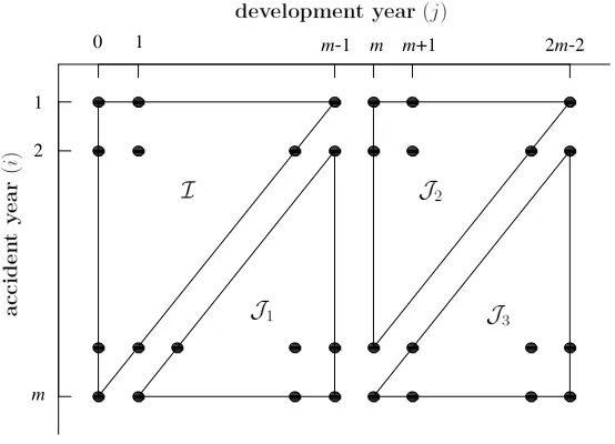
reserve, our recommendation is to condition on the actual numbers of claims, and use (1). For the IBNR reserve it is necessary first to construct predictions of future numbers of reported claims (using the CLM). Using the notation of Verrall et al. (2010) and Mart´ınez-Miranda et al. (2011), we consider predictions over the following triangles (which are illustrated in Figure 1):

J1 ={i= 2, . . . , m;j = 0, . . . , m−1 so i+j =m+ 1, . . . ,2m−1} J2 ={i= 1, . . . , m;j =m, . . . ,2m−1 so i+j =m+ 1, . . . ,2m−1} J3 ={i= 2, . . . , m;j =m, . . .2m−1 so i+j = 3m, . . . ,3m−2}.

Figure 1: Index sets for aggregate claims data, assuming a maximum delay

m−1.

Note that the standard CLM would produce forecasts over onlyJ1. If the

CLM is being used, it is therefore necessary to construct tail factors in some way. For example, this is sometimes done by assuming that the run-off will follow a set shape, thereby making it possible to extrapolate the development factors. In contrast, DCL provides also the tail over J2∪ J3 using the same

over all parts of the data, and uses the same assumptions concerning the delay mechanisms producing the data throughout.

In Section 4.1 we set out the way the outstanding claims can be estimated, ignoring the tail, and in Section 4.2 we consider also the tail.

4.1

Estimation of outstanding claims ignoring the tail

The estimates of outstanding claims using the CLM can be constructed using XbCL

ij = αbeiβbej for (i, j) ∈ J1. There are a number of possibilities that

could be used to estimate Xij (for (i, j) ∈ J1) using the assumptions in

section 2. For these assumptions, the estimates will be the sum of an RBNS component and an IBNR component. We consider first using (1) and (2) in order to show the connection with the CLM. It is possible to use either the actual numbers of claims or the fitted values for the RBNS component. Thus, there are two possible estimates, which we denote by Xb_ijrbns(1), based on (1), and Xbijrbns(2), based on (2):

b

Xijrbns(1) = j

X

l=i−m+j

Ni,j−lbπlbµbγi (13)

and

b

X_ijrbns(2) =

j

X

l=i−m+j

b

Ni,j−lbπlbµbγi (14)

where Nbij =αbiβbj. The IBNR component always uses (2):

b

Xijibnr =

i−m_X+j−1

l=0

b

Ni,j−lbπlµbbγi. (15)

Theorem 1 For (i, j)∈ J1, define

b

XCL

ij = αbeibeβj

b

X_ijrbns(2) =

j

X

l=i−m+j

b

Ni,j−lbπlµbbγi

b

Xijibnr =

i−m_X+j−1

l=0

b

Ni,j−lbπlµbbγi

where

b

αibµbγi =αebi, j

X

l=0

b

βj−lbπl =βebj.

Then XbCL ij =Xb

rbns(2)

ij +Xbijibnr.

Proof

b

Xijrbns(2)+Xb ibnr ij =

j

X

l=i−m+j

b

Ni,j−lbπlbµbγi+

i−m_X+j−1

l=0

b

Ni,j−lbπlµbbγi

=

j

X

l=0

b

Ni,j−lbπlbµbγi

=

j

X

l=0

b

αiβbj−lπblµbbγi

=

j

X

l=0

(α_biµbbγi)βbj−lbπl

= α_ebi j

X

l=0

b

βj−lπbl

= α_ebiβebj =XbijCL.

the tail (defined over J2∪ J3) will be exactly the same as the standard CLM

estimate. Thus, we have shown that this can be considered as another specifi-cation of a stochastic model for the CLM. Note it is close to the first moment specifications defined in Section 2, which is based on detailed assumptions about the mechanisms generating the data, and is not simply defined in order to provide the same estimates as the CLM.

While it would be possible to simply use the specification used in the above theorem (i.e. use equation (2) together with the fitted numbers of claims), we believe that this is not the best thing to do. We believe that it is better to use the actual numbers of claims for the RBNS reserve estimate, rather than the fitted values. Thus, although our preferred model is similar in structure to the (detailed) CLM, it will not give the same results. We be-lieve that the estimates from our model are preferable, and this could be seen as a (mild) criticism of the CLM, although the differences in the estimates will probably not be large. More importantly, we believe that our model is also superior to the basic CLM since all the parameters have a real inter-pretation. For this reason, when it is necessary to make alterations to the parameter estimates, or to move on to more sophisticated models within the same basic framework, we believe that our model will be preferable. When setting reserves, assessing capital requirements or proving adequate solvency conditions, we believe that it is easier to justify expert intervention on pa-rameters that relate to real underlying factors. The development factors for the CLM applied to aggregated payments represent a complex combination of these underlying factors, and it is therefore more difficult to show that intervention to alter their values is based on well-formulated arguments and is not simply ad hoc, or (even worse) designed simply to get the “right” answer.

4.2

DCL including the run-off

Although the CLM does not include estimates for development years be-yond the maximum already observed, it is necessary to include these when setting a reserve. In the context of the CLM, this is often done by fit-ting a curve of some form to the development year parameters. The tail consists of estimates over J2 ∪ J3 and these are given quite naturally by

b

Rtail ₌P

(i,j)∈J2∪J3

min(j,d)

X

l=0

b

Ni,j−lbπlµbbγi.

When estimating the tail we have implicitly assumed that we have seen a full run-off of the first underwriting year. If this is not the case our tail estimation underestimates the real tail and further adjustments might be necessary.

5

One statistical model with the DCL first

moments

Many mathematical statistical models exist with the first moment structure of the DCL. In this section we go through the simplest and perhaps most important one: the one payment per reported claim model. The purpose of introducing a mathematical statistical DCL model is to be able to understand the distribution of the outstanding liabilities. With the selected estimation procedure of the first moment parameters of DCL, the statistical model will not affect the best estimate of these outstanding liabilities, but only their distribution. Of course, it is often the case that insurance claims give rise to more than one payment, or even to zero payments. However, the distribu-tional assumptions in this section will be an approximation to the underlying true distribution. The one payment assumption shoud give a good approx-imation to the true underlying distribution that will be difficult to improve upon in practice. Even if full information on the historical payment process was available, the incorporation of this information into the statistical model would imply understanding the non-trivial time series correlation between payments in the payment process. If this correlation is not well modelled, the payment process (even when observed) in the statistical model might not improve the approximation to the underlying distribution. And also, in general when more information is included in an attempt to improve on the approximation to the DCL, care should be taken to ensure that the extra information is not counter-weighted by the often unavoidable added model error introduced from modelling this extra information. In short, we intro-duce the simple one payment per claim model believing this to be a good first approximation to the underlying distribution, because the payment process in practice often is dominated by one of the payments.

payments are gamma distributed. This would be simple to adjust if neces-sary, but the gamma distribution is a convenient distribution to start with. The approach can be easily generalised to other distributions, for example those with heavier pareto tails that might be appropriate for some data sets. Another adjustment of the severity distribution could be to consider a mixed model of for example a gamma distribution and the point measure at zero in order toallow for the distributional properties stemming from the possibility that some of the reported claims are indeed zero claims. However, such a zero-claim approach would include an extra parameter in the volatility esti-mation process below complicating our estiesti-mation procedure and exposition and we have therefore decided not to include it this study.

The model of Verrall et al. (2010) and Mart´ınez-Miranda et al. (2011) was constructed by considering three stochastic components: the settlement delay, the individual payments and the reported counts. Here we consider a very similar model which is formulated under the assumptions given below.

D1. The counts: The counts Nij are independent random variables from a

Poisson distribution with multiplicative parametrization E[Nij] =αiβj

and identification (Mack 1991), Pm_j=0−1βj = 1.

D2. The RBNS delay. Given Nij, the distribution of the numbers of paid

claims follows a multinomial distribution, so that the random vector (N_ijpaid₀ , . . . , N_ijdpaid)∼ Multi(Nij;p0, . . . , pd), for each (i, j)∈ I, where d

denotes the maximum delay (d≤m−1). Let p= (p0, . . . , pd) denote

the delay probabilities such that Pd_l=0pl = 1 and 0< pl <1,∀l.

D3. The payments. The individual paymentsY_ijl(k)are mutually independent with distributionsfi. Let µi and σi2 denote the mean and the variance

for each i = 1, . . . , m. Assume that µi = µγi, with µ being a mean

factor and γi the inflation in the accident years. Also the variances are

σ2

i =σ2γi2 withσ2being a variance factor. Note that we are considering

a more general situation than Verrall et al. (2010) by assuming that the distribution depends on the accident year, but a slightly less general case than in Section 2 where the mean also depended on the payment delay. In fact, the model of Verrall et al. (2010) assumes that γi = 1,

∀i= 1, . . . , m.

assumed that the claims are settled with a single payment or maybe as “zero-claims” (to deal with such a situation, it is necessary to consider a mixed-type distribution for the individual payments following the arguments in Verrall et al. (2010)).

Under the above assumptions the conditional mean ofXij becomes

E[Xij|ℵm] =

min(_Xj,d)

l=0

Ni,j−lplµγi, (16)

and therefore the unconditional mean is

E[Xij] =αiµγi

min(_Xj,d)

l=0

βj−lpl. (17)

Note that these first moments has the DCL mean structure defined in (1) and (2) by replacing the parameters π = {πl : l = 0, . . . , m−1} with no

restrictions on the values of πl by the probabilities p = {pl : l = 0, . . . , d},

where Pd_l=0pl= 1 and 0< pl <1,∀l.

In general, we would expect the values of these parameters,pandπ, to be very similar and that the predictions from the models would also be similar. Although these parameter estimates (p_bj and bπj) will be very similar (by

definition), there may be differences for the longer reporting delays, which will affect the estimates of the reserves. This is illustrated in the example in Section 6.

Now using assumptions D1-D4 and arguments from Verrall et al. (2010) we can deal with higher moments calculations and provide the variance of the aggregated payments. Specifically the conditional variance of Xij is

approx-imately proportional to the mean. Since we have introduced the parameters

γi, the dispersion parameter in this case depends on i.

V[Xij|ℵm] ≈

σ2

i +µ2i

µi

E[Xij|ℵm] (18)

= γi

σ2 _+µ2

µ E[Xij|ℵm] (19)

= ϕiE[Xij|ℵm]. (20)

where ϕi =γiϕ and ϕ = σ

2

+µ2

µ . This means that an over-dispersed Poisson

5.1

Estimation of the reporting delay

We consider first the mean specification given in (2), and then discuss how to modify the results in order to provide estimates for the parameters in (17). So first we estimate the parameters π ={πl :l = 0, . . . , m−1} by

solving the linear system defined in (7). Letπ_b denote such solution with the individual elements denoted by _bπl, l = 0, . . . , m−1. Note that the values πbl

could be negative and they could also sum to more than 1.

Considering the parameters in (17), there are a number of ways in which the parameters could be estimated including a constrained estimation pro-cedure. However, we use a simple method, which we believe will provide reasonable estimates in most cases. For this, we estimate the maximum delay period, d, by counting the number of successive π_bl ≥ 0 such that

Pd−1

l=0 bπl < 1 ≤ Pd_l=0bπl. Then the estimated delay parameters in (2) are

defined as

b

pl = bπl, l = 0, . . . , d−1, (21)

b

pd = 1−

d−1

X

l=0

b

pl. (22)

Thus, p_b= (p_b0, . . . ,pbd−1,1−Pd_l=0−1pbl).

5.2

Estimation of the parameters of the distribution

of individual payments

The estimation of the mean of the distribution of individual payments, in-cluding the parameters which measure the inflation in the accident years comes from equations (8) and (9) above.

The estimation of the variances,σ2

i (i= 1, . . . , m) can be provided using

the estimator proposed by Verrall et al. (2010). Specifically we estimate the overdispersion parameter ϕ by

b

ϕ = 1

n−(d+ 1)

X

i,j∈I

(Xij −XbijDCL)2

b

XDCL

ij bγi

, (23)

where n=m(m+ 1)/2 andXbDCL

ij is the DCL estimate of E[Xij|ℵm] defined

by XbDCL ij =

Pmin(j,d)

payment can be estimated by

b

σ2i =bσ2bγi2 (24)

for each i= 1, . . . , m, where_bσ2 _{=µbϕb−µb}2_.

6

Empirical illustration

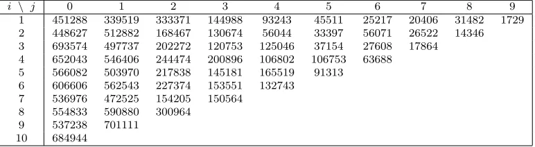
This paper uses the same motor data as Verrall et al. (2010) and Mart´ınez-Miranda et al. (2011), which originates from the general insurer RSA and is based on a portfolio of motor third party liability policies. The data available consists of two incremental run-off triangles of dimensionm = 10, one for re-ported counts,Nij, and one for aggregated payments,Xij, wherei= 1, . . . , m

denotes the accident year and j = 0, . . . , m−1 is the development year. The data are shown in Tables 1 and 2, respectively.

i \ j 0 1 2 3 4 5 6 7 8 9 1 6238 831 49 7 1 1 2 1 2 3 2 7773 1381 23 4 1 3 1 1 3 3 10306 1093 17 5 2 0 2 2 4 9639 995 17 6 1 5 4 5 9511 1386 39 4 6 5 6 10023 1342 31 16 9 7 9834 1424 59 24 8 10899 1503 84 9 11954 1704 10 10989

Table 1: Run-off triangle of number of reported claims,Nij

i \ j 0 1 2 3 4 5 6 7 8 9

1 451288 339519 333371 144988 93243 45511 25217 20406 31482 1729 2 448627 512882 168467 130674 56044 33397 56071 26522 14346 3 693574 497737 202272 120753 125046 37154 27608 17864 4 652043 546406 244474 200896 106802 106753 63688 5 566082 503970 217838 145181 165519 91313

6 606606 562543 227374 153551 132743 7 536976 472525 154205 150564

8 554833 590880 300964 9 537238 701111

10 684944

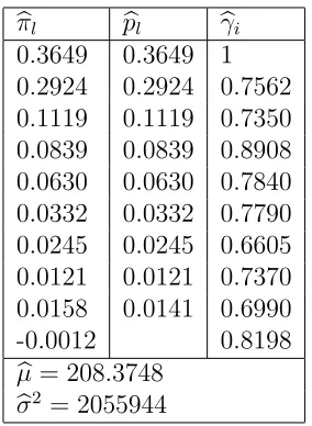
Table 3 gives the estimates of the parameters from the motor data for the model (D1-D4) .

Point forecasts of the reported but not settled (RBNS) reserve and the incurred but not reported (IBNR) reserve can now be constructed along the lines of Verrall et al. (2010) Mart´ınez-Miranda et al. (2011). The cash flow by calendar year is computed by summing the point forecasts Xbij along the

diagonals of J1. Table 4 shows the RBNS and IBNR reserve and also the

total (RBNS+IBNR) forecasts. As a benchmark for comparison purposes, the predicted chain ladder reserve (denoted by CLM) is also shown in the last column of Table 4.

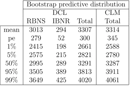
To derive the predictive distribution of the RBNS and IBNR reserves we consider bootstrap methods as proposed by Mart´ınez-Miranda et al. (2011). The bootstrap technique allows us to take into account the uncertainty of the parameters in the assumed model. The summary statistics from the RBNS and IBNR cash-flows, estimated by these bootstrap method are shown in Table 5. The root mean square error of prediction, commonly known as the prediction error, is denoted by “pe”. We also compare the cash-flows derived from the proposed DCL method with the results from the BCL package in R by Gesmann et al. (2011) which implements the bootstrap method of England and Verrall (1999) and England (2002) for the CLM in Table 4.

7

Conclusions

Acknowledgement

This research was financially supported by a Cass Business School Pump Priming Grant. The first author is also supported by the Spanish Ministerio de Ciencia e Innovaci´on, Project MTM2008-03010. We would like to thank for helpful comments from attenders of the Astin Colloquia 2011 held in Madrid. In particular we would like to thank Mario W¨uthrich for pointing out that our tail estimator in some situations underestimates.

8

References

Bj¨orkwall, S., H¨ossjer, O. & Ohlsson, E. (2009a) Non-parametric and Para-metric Bootstrap Techniques for Arbitrary Age-to-Age Development Factor Methods in Stochastic Claims Reserving. Scandinavian Actuar-ial Journal, 4, 306-331.

Bj¨orkwall, S., H¨ossjer, O. & Ohlsson, E. (2009b) Bootstrapping the separa-tion method in claims reserving. ASTIN Bulletin 40(2), 845–869.

Bryden, D. and Verrall, R.J. (2009) Calendar year effects, claims inflaton and the Chain-Ladder technique. Annals of Actuarial Science 4, 287-301.

B¨uhlmann, H., Schnieper, R. and Straub, E. (1980): Claims reserves in casualty insurance based on a probability model. Mitteilungen der Vereinigung Schweizerischer Versicherungsmathematiker.

England, P. (2002) Addendum to “Analytic and Bootstrap Estimates of Prediction Error in Claims Reserving”. Insurance: Mathematics and Economics 31, 461–466.

England, P. and Verrall, R. (1999) Analytic and Bootstrap Estimates of Prediction Error in Claims Reserving. Insurance: Mathematics and Economics 25, 281–293.

England, P. and Verrall, R. (2006) Predictive Distributions of Outstanding Liabilities in General Insurance. Annals of Actuarial Science, 1(2), 221–270.

Gesmann, M., Wayne, Z. and Murphy, D. (2011) R-package ”ChainLadder” version 0.1.4-3.4 (22 March, 2011). URL:

http://code.google.com/p/chainladder/

Kremer, E. (1985)Einf¨uhrung in die Versicherungsmathematik. G¨ottingen: Vandenhoek & Ruprecht.

Kuang, D., Nielsen, B.and Nielsen, J.P. (2008a) Identification of the age-period-cohort model and the extended chain-ladder model. Biometrika

95, 979–986.

Kuang, D., Nielsen, B. and Nielsen, J.P. (2008b) Forecasting with the age-period-cohort model and the extended chain-ladder model. Biometrika

95, 987–991.

Kuang, D., Nielsen, B. and Nielsen, J.P. (2009) Chain Ladder as Maximum Likelihood Revisited. Annals of Actuarial Science 4, 105–121.

Kuang, D., Nielsen, B. and Nielsen, J.P. (2011) Forecasting in an extended chain-ladder-type model. Journal of Risk and Insurance 78, 345–359.

Mack, T. (1991) A simple parametric model for rating automobile insurance or estimating IBNR claims reserves. ASTIN Bulletin, vol. 39, 35–60.

Mart´ınez-Miranda, M.D., Nielsen, B., Nielsen, J.P. and Verrall, R. (2011) Cash flow simulation for a model of outstanding liabilities based on claim amounts and claim numbers. ASTIN Bulletin, 41(1), 107–129.

Norberg, R., (1986): A contribution to modelling of IBNR claims. Scandi-navian Actuarial Journal, 3, 155–203.

Norberg, R., (1993): Prediction of outstanding liabilities in non-life insur-ance. ASTIN Bulletin, 23(1), 95–115.

Pinheiro, P.J.R., Andrade e Silva, J.M. and Centeno, M.d.L. (2003) Boot-strap Methodology in Claim Reserving. Journal of Risk and Insurance

4, 701–714.

R Development Core Team (2011) R: A Language and Environment for Statistical Computing. R Foundation for Statistical Computing, Vienna (Austria). URL: http://www.R-project.org

Renshaw, A. E. and Verrall, R. (1998): A stochastic model underlying the chain ladder technique. British Actuarial Journal 4, 903–923.

Taylor, G. (1977) Separation of inflation and other effects from the distri-bution of non-life insurance claim delays. ASTIN Bulletin 9, 217–230.

Verrall, R. (1991) Chain ladder and Maximum Likelihood. Journal of the Institute of Actuaries 118, 489–499.

Verrall, R. (2000) An Investigation into Stochastic Claims Reserving Models and the Chain-Ladder Technique. Insurance: Mathematics and Eco-nomics 26, 91–99.

Verrall, R., Nielsen, J.P. and Jessen, A. (2010) Including Count Data in Claims Reserving. ASTIN Bulletin 40(2), 871–887..

W¨uthrich, M. and Merz, M. (2008). Stochastic Claims Reserving Methods in Insurance. Wiley.

b

πl pbl bγi

0.3649 0.3649 1 0.2924 0.2924 0.7562 0.1119 0.1119 0.7350 0.0839 0.0839 0.8908 0.0630 0.0630 0.7840 0.0332 0.0332 0.7790 0.0245 0.0245 0.6605 0.0121 0.0121 0.7370 0.0158 0.0141 0.6990 -0.0012 0.8198

b

µ= 208.3748

b

σ2 _{= 2055944}

Table 3: Estimated parameters for motor data: the parameters _bπl (l =

0, . . . ,9), the delay probabilities p_bl (l = 0, . . . , d = 8), the inflation

DCL

Future RBNS IBNR Total CLM 1 1260 97 1357 1354 2 672 83 754 754 3 453 35 489 489 4 292 26 319 318 5 165 20 185 185 6 103 12 115 115

7 54 9 63 63

8 30 5 36 36

9 0 5 5 2

10 1 1

11 0.6 0.6

12 0.4 0.4

13 0.2 0.2

14 0.1 0.1

15 0.06 0.06 16 0.03 0.03 17 0.01 0.01

Total 3030 296 3326 3316

Bootstrap predictive distribution

DCL CLM

RBNS IBNR Total Total mean 3013 294 3307 3314

pe 279 52 300 345 1% 2415 198 2661 2588 5% 2575 215 2821 2780 50% 2995 289 3291 3287 95% 3505 389 3813 3911 99% 3649 425 4020 4061