Verification and validation of a theoretical model of a direct drive valve-controlled electrohydrostatic actuator for primary flight control

(1)

Theses Thesis/Dissertation Collections

5-1-2012

Verification and validation of a theoretical model of

a direct drive valve-controlled electrohydrostatic

actuator for primary flight control

Heather Hussain

[email protected]

Follow this and additional works at:http://scholarworks.rit.edu/theses

Recommended Citation

(2)

Direct Drive Valve-Controlled Electrohydrostatic Actuator

for Primary Flight Control

Thesis

by

Heather Syeda Hussain

A Thesis Submitted in Partial Fulfillment of the Requirements for the Degree of Master of Science in Mechanical Engineering

Supervised by

Associate Professor Dr. Agamemnon Crassidis Department of Mechanical Engineering

Kate Gleason College of Engineering Rochester Institute of Technology

Rochester, New York May 2012 Approved by:

Dr. Agamemnon Crassidis, Associate Professor

Thesis Advisor, Department of Mechanical Engineering

Dr. Jason Kolodziej, Assistant Professor

Committee Member, Department of Mechanical Engineering

Dr. Marca Lam-Anderson, Instructional Faculty

Committee Member, Department of Mechanical Engineering

Dr. Alan Nye, Department Representative

(3)

Rochester Institute of Technology Kate Gleason College of Engineering

Title:

Verification and Validation of a Theoretical Model of a Direct Drive Valve-Controlled Electrohydrostatic Actuator for Primary Flight Control

I, Heather Syeda Hussain, hereby grant permission to the Wallace Memo-rial Library to reproduce my thesis in whole or part.

(4)

Dedication

(5)

Acknowledgments

It is with immense gratitude that I acknowledge the support of Moog Aircraft Group. I consider it an honor to work with engineers Rick Fosdick

and David Gawelo. Technician support was also greatly appreciated by Garry Handzlik.

(6)

Abstract

Verification and Validation of a Theoretical Model of a Direct Drive Valve-Controlled Electrohydrostatic Actuator for Primary Flight

Control Thesis

Supervising Professor: Dr. Agamemnon Crassidis

(7)

List of Figures

1.1 High Level Valve-Controlled Hydraulic Actuator Diagram . 1

1.2 Conventional Servovalve-Controlled Hydraulic Actuator . . 2

1.3 High Level Electrohydrostatic Actuator Diagram . . . 2

1.4 Electrohydrostatic Actuator . . . 3

1.5 Hydraulic Bays of Lockheed P-7A ASW . . . 4

1.6 Airbus A380 Flight Control Surfaces . . . 5

1.7 Airbus A380 Actuation Configuration . . . 6

1.8 Schematic of FBW Hydraulic Actuator, EHA, and EBHA . . 7

1.9 Integrated Actuation Package . . . 9

1.10 Integrated Actuation Package Schematic . . . 10

2.1 Linear Force Motor Direct Drive Valve . . . 14

2.2 Linear Force Motor . . . 15

2.3 Four-way Spool Valve Hydraulic Schematic . . . 18

2.4 Experimental Valve Test Set Up . . . 19

2.5 Experimental Frequency Response of DDV . . . 21

2.6 0.5V Amplitude Frequency Response . . . 21

(12)

2.15 Experimental and Theoretical Frequency Response - All . . 26

2.16 Final Theoretical Valve Model Open Loop Response . . . . 27

2.17 Final Theoretical Valve Model - Small and Large Amp . . . 28

2.18 Valve Leakage Validation . . . 29

2.19 Valve Flow Gain Validation . . . 29

2.20 Valve Position Validation . . . 30

2.21 Valve Pressure Gain Validation . . . 30

3.1 DDV Actuator Schematic . . . 31

3.2 LuGre Friction Model . . . 34

3.3 Actuator Piston-Cylinder Theoretical Bode Plot . . . 38

3.4 DDV Actuator - Low Frequency Sinusoidal Command . . . 40

3.5 DDV Actuator - No Load Rate . . . 41

3.6 DDV Actuator - NLR Variables . . . 42

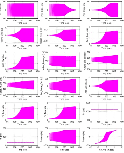
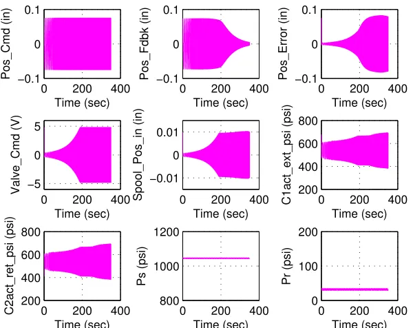
3.7 DDV Actuator - Small Amp Frequency Response Variables . 45 3.8 DDV Actuator - Experimental Small Amp FR Variables . . . 46

3.9 DDV Actuator - Theoretical Small Amp FR Variables . . . . 46

3.10 DDV Actuator - Input and Output Small Amp FR Nonlinear 47 3.11 DDV Actuator - Small Amp NL Mag, Phase, and Coherence 47 3.12 DDV Actuator - Input and Output Small Amp FR Linear . . 48

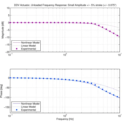
3.13 DDV Actuator - Small Amp Lin Mag, Phase, and Coherence 48 3.14 DDV Actuator - Small Amp FR Validation . . . 49

3.15 DDV Actuator - Large Amp Frequency Response Variables . 50 3.16 DDV Actuator - Experimental Large Amp FR Variables . . . 51

3.17 DDV Actuator - Theoretical Large Amp FR Variables . . . . 51

(13)

3.21 DDV Actuator - Large Amp Lin Mag, Phase, and Coherence 53

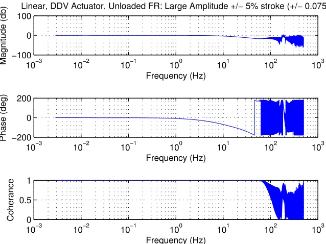
3.22 DDV Actuator - Large Amp FR Validation . . . 54

3.23 Experimental DDV Actuator Test Set Up . . . 55

3.24 Top View of DDV Actuator . . . 55

4.1 Performance Mapping of Hydraulic Pump . . . 59

4.2 Pump Output Flow - Speed . . . 59

4.3 Pump Output Flow - Pressure . . . 60

4.4 Flow Loss - Speed . . . 60

4.5 Flow Loss - Pressure . . . 61

4.6 Volumetric Pump Efficiency - Speed . . . 61

4.7 Volumetric Pump Efficiency - Pressure . . . 62

4.8 Pump Torque Output - Speed . . . 62

4.9 Pump Torque Output - Pressure . . . 63

4.10 Torque Loss and Optimization Convergence - Speed . . . 63

4.11 Torque Loss and Optimization Convergence - Pressure . . . 64

4.12 Pump Optimization Cost Function Value . . . 64

4.13 Torque Efficiency - Speed . . . 65

4.14 Torque Efficiency - Pressure . . . 65

4.15 Overall Pump Efficiency - Speed . . . 66

4.16 Overall Pump Efficiency - Pressure . . . 66

4.17 Experimental Pump Test Set Up - CAD . . . 67

4.18 Pump Hydraulic Connections and Plumbing . . . 67

5.1 Electrohydrostatic Actuator Hydraulic Schematic . . . 68

5.2 Velocity and Current PI Loops . . . 70

(14)

5.6 EHA - Small Amp Frequency Response Variables . . . 78

5.7 EHA - Experimental Small Amp FR Variables . . . 79

5.8 EHA - Theoretical Small Amp FR Variables . . . 79

5.9 EHA - Input and Output Small Amp FR Nonlinear . . . 80

5.10 EHA - Small Amp NL Mag, Phase, and Coherence . . . 80

5.11 EHA - Input and Output Small Amp FR Linear . . . 81

5.12 EHA - Small Amp Lin Mag, Phase, and Coherence . . . 81

5.13 EHA - Small Amp FR Validation . . . 82

5.14 EHA - Large Amp Frequency Response Variables . . . 83

5.15 EHA - Experimental Large Amp FR Variables . . . 84

5.16 EHA - Theoretical Large Amp FR Variables . . . 84

5.17 EHA - Input and Output Large Amp FR Variables . . . 85

5.18 EHA - Large Amp NL Mag, Phase, and Coherence . . . 85

5.19 EHA - Input and Output Large Amp FR Linear . . . 86

5.20 EHA - Large Amp Lin Mag, Phase, and Coherence . . . 86

5.21 EHA - Large Amp FR Validation . . . 87

5.22 Experimental EHA Test Set Up . . . 88

5.23 Disconnected Load Actuator . . . 88

6.1 Hybrid (DDV-EHA) Actuator Schematic . . . 89

6.2 Simulink Sump-Pump Model . . . 91

6.3 Hybrid - Low Frequency Sinusoisal Command . . . 95

6.4 Hybrid - No Load Rate . . . 96

6.5 Hybrid - NLR Variables . . . 97

6.6 Hybrid - Experimental Small Amp FR Variables . . . 99

6.7 Hybrid - Theoretical Small Amp FR Variables . . . 100

6.8 Hybrid - Input and Output Small Amp FR Nonlinear . . . . 101

6.9 Hybrid - Small Amp NL Mag, Phase, and Coherence . . . . 101

(15)

6.11 Hybrid - Experimental Large Amp FR Variables . . . 103

6.12 Hybrid - Theoretical Large Amp FR Variables . . . 104

6.13 Hybrid - Input and Output Large Amp FR Nonlinear . . . . 105

6.14 Hybrid - Large Amp NL Mag, Phase, and Coherence . . . . 105

6.15 Hybrid - Large Amp FR Validation . . . 106

6.16 Test Rig CAD for DDV-EHA Experimental Test Set up . . . 107

6.17 DDV-EHA Experimental Set up . . . 107

7.1 DDV Actuator and Hybrid - Small Amp FR Comparison . . 109

7.2 Small Amp FR Comparison . . . 110

7.3 DDV Actuator and Hybrid - Large Amp FR Comparison . . 110

7.4 Large Amp FR Comparison . . . 111

7.5 Load Hold Power Analysis . . . 113

7.6 High-Rate No-Load Power Analysis . . . 114

7.7 Power Output Analysis for Rate Limited Curves . . . 115

7.8 Power Input Analysis for Rate Limited Curves . . . 116

7.9 Efficiency Analysis for Rate Limited Curves . . . 117

7.10 Power Input Analysis at 1% NLR . . . 118

7.14 Increased Pump Efficiency Analysis for Rate Limited Curves 120 A.1 Linear DDV Actuator Theoretical Simulink Model . . . 130

A.2 Nonlinear DDV Actuator Theoretical Simulink Model . . . 131

A.3 PI Control of DC Brushless Motor Model . . . 132

(16)

Nomenclature

Acronyms

2H/2E Two Hydraulic, Two Electric page 5

APU Auxiliary Power Unit page 6

BLDC Brushless Direct Current page 9

CL Closed Loop page 9

DC Direct Current page 70

DDV Direct Drive Valve page 11

DDV-EHA Direct Drive Valve-Controlled Elec-trohydrostatic Actuator

page 11

EBHA Electrical Back-up Hydrostatic

Actu-ator

page 7

EHA Electrohydrostatic Actuator page 2

EHSV Electrohydraulic Servovalve page 9

EMF Electromotive Force page 71

FBW Fly By Wire page 2

IPA Integrated Actuator Package page 9

LVDT Linear Variable Differential

Trans-ducer

page 32

MEA More Electric Aircraft page 3

MTBF Mean Time Between Failure page 6

NLR No Load Rate page 41

PBW Power By Wire page 2

(17)

PI Proportional-Integral page 69

PWM Pulse Width Modulation page 32

UUT Unit Under Test page 35

VCA Valve-Controlled Actuator page 1

Equation Variables

Hydraulic Fluid Bulk Modulus lbf/in2 _{page 35}

P Differential Pressure lbf/in2 page 16

xact Actuator Position Error in page 32

 Specific Heat Capacity Ratio - page 92

⌫f luid Kinematic Viscosity in2/s page 57

! Motor Speed rad/s page 57

!n Natural Frequency of Valve rad/s page 16

⇢hyd Hydraulic Fluid Density slug/in3 page 17

0 Friction Stiffness Coefficient lbf/in page 33

1 Friction Damping Coefficient lbf-s/in page 33

2 Friction Viscous Coefficient lbf-s/in page 33

⌧p Corner Frequency of Additional Pole rad/s page 16

⇣ Damping Coefficient of Valve - page 16

⇣ Damping Coefficient of the

Cylinder-Fixture

- page 37

A Area of Flow in2 page 17

Apist Piston Area in2 page 35

B Damping Coefficient lbf-s/in page 33

B Rotational Damping Coefficient in-lbf/s page 71

(18)

cp Specific Heat Capacity Constant

Pres-sure

J/kg-K page 92

cs Specific Heat Capacity Constant

Vol-ume

J/kg-K page 92

Cinlbf2N m Conversion Factor Nm/in-lbf page 112

Dp Pump Displacement in3/rad page 57

eispool Valve Input Command V page 32

emag Frequency Response Magnitude Error - page 19

ephase Frequency Response Phase Error - page 19

Fc Coulomb Friction lbf page 33

Ff Friction Force lbf/in page 33

Fs Viscous Friction lbf page 33

Factout Actuator Force Output lbf page 112

FLoad External Load Force lbf/in page 33

GV Valve Flow Gain p1

K page 17

GP I PI Controller - page 69

i Motor Current A page 70

J Cost Function Valve - page 19

J Rotational Inertial Mass in-lbf/s2 page 71

Jmtr Motor Intertia in-lbf/s2 page 71

Jpump Pump Inertia in-lbf/s2 page 71

K Coefficient of Flow Gain lbf-s/in5 page 17

Kb Motor Back EMF Constant V-s/rad page 70

KD Derivative Gain 1/s page 70

KI Integral Gain s page 69

KP Proportional Gain - page 32

Ks Spring Constant lbf/in page 33

KT Motor Torque Constant in-lbf/Amp page 70

(19)

Khyd Hydraulic Stiffness lbf/in page 37

Kloss Pump Flow Loss Coefficient in5/s-lbf page 57

L Motor Inductance Henry page 71

Mt Total Mass slug page 33

Mf ix Fixture Mass slug page 37

Mpist Piston Mass slug page 37

P Pressure lbf/in2 page 92

PR Return Pressure lbf/in2 page 17

PS Supply Pressure lbf/in2 page 17

Patm Atmospheric Pressure lbf/in2 page 92

PC1ext Cylinder Extend Pressure in page 35

PC2ret Cylinder Retract Pressure in page 36

PCV Cylinder Pressure lbf page 35

PgasR Pressure of Gas in Return

Accumula-tor

lbf/in2 _{page 93}

PgasS Pressure of Gas in Supply

Accumula-tor

lbf/in2 _{page 93}

Pgas Accumulator Gas Pressure lbf/in2 page 92

Pin Electrical Input Power Watt page 111

Pout Actuator Power Output Watt page 112

Ppr Preload Pressure of Fluid lbf/in2 page 92

Q Volumetric Flow Rate in3/s page 16

QC1ext Cylinder Extend Flow in

3_/s _{page 17}

QC2ret Cylinder Retract Flow in

3_/s _{page 17}

QP rDDV Valve Return Flow in

3_/s _{page 93}

QP sDDV Valve Supply Flow in

3_/s _{page 93}

Qpumpin Pump Flow Into Accumulator in

(20)

Tideal Ideal Torque in-lbf page 57

Tload External Torque Load in-lbf page 71

V Actuator Piston Velocity in/s page 35

V Volume in3 page 92

V0 Volume of One Side of Piston

Cham-ber

in3 _{page 37}

va Voltage Input V page 71

VF Accumulator Fluid Volume in3 page 92

vp Actuator Piston Velocity in/s page 33

vs Stribeck Velocity in/s page 33

Vt Total Volume of the Piston Chamber in3 page 37

Vacc Accumulator Volume in3 page 92

Vcmd Valve Input Command V page 16

VgasR Volume of Gas in Return

Accumula-tor

in3 _{page 93}

VgasS Volume of Gas in Supply

Accumula-tor

in3 _{page 93}

Vgas Accumulator Gas Volume in3 page 92

Vpr Preload Volume of Fluid in3 page 92

wslot Width of Spool Slot in page 17

xactcmd Actuator Input Position Command in page 32

xactf dbk Actuator Position Feedback in page 32

xspool Spool Position in page 16

(21)

Chapter 1

Introduction

Modern aircraft are combining conventional servovalve controlled hy-draulic actuation and electrically signaled hyhy-draulic actuation to achieve a more electric aircraft flight control actuation system.

Figure 1.1: High Level Conventional Servovalve-Controlled Hydraulic Actuator Diagram [1]

(22)

2

Fault Diagnosis of Electrohydraulic Servoactuators

A Benchmark Study

-A. Salas, -A. Rodriguez and S. X. Ding

Institute for Automatic Control and Complex Systems (AKS)

Bismarckstr. 81, 47057 Duisburg

University of Duisburg-Essen, Germany

Abstract

—This paper presents a benchmark study on fault

diagnosis of electrohydraulic servoactuators (EHSA). EHSA

are considered to be affected by faults and disturbances.

The linear mathematical model of the EHSA is given. Two

different design methods for fault diagnosis are studied. The

first method considers the strategy of parity space design, and

observer-based implementation, in which a perfect disturbance

decoupling is achieved. The second method considers the linear

EHSA model with polytopic uncertainties in order to design

a residual signal using fault detection filter (FDF) theory, and

to calculate a threshold. Linear matrix inequalities (LMI) are

used to obtain the problem solutions.

I.

INTRODUCTION

Electrohydraulic servoactuators (EHSA) are divided in two

parts, a servovalve and a cylinder, see Fig. 1. The

math-ematical model of EHSA has been widely studied [1]. In

this paper fault diagnosis of EHSA is studied. Two different

design objectives are considered:

•

Perfect disturbance decoupling

•

Polytopic uncertainties

i

SV

Servovalve

Cylinder

d(t)

Control

x

p

!p

Fig. 1.

Electrohydraulic Servoactuator

Disturbance decoupling, also known as unknown input

de-coupling, has been studied in the last decades. One of

the first unknown input residual generation schemes was

proposed by Wünnenberg and Frank in [12]. The idea

behind the unknown input decoupling strategy is simple

and clear: if the generated residual signals are independent,

not only of the inputs and initial conditions, but also the

unknown inputs, then they can be directly used as a fault

indicator. Several papers have been published for disturbance

decoupling. In [7], [13] is presented the design of a bank

of observers, where each observer is sensible to only one

fault but robust to the other faults and disturbances. Paper

[6] presents an optimally robust residual generation and

evaluation in frequency domain. The approach parity space

design, observed based implementation has been applied

for the vehicle lateral dynamics [9], [10], whose mainly

purpose is to handle with uncertainties and isolate faults.

Polytopic linear models (PLM) can be also considered as

nonlinear models built with a number of local linear models,

each linear model is linearized in a different operating point

[11]. Some papers have been published using polytopic

uncertainties. In [8] fault diagnosis is presented to decouple

modeling errors using polytopic unknown input observers

(UIO). Paper [15] presents a robust fault detection filter

(RFDF) using

H

filtering.

Section II of this paper presents the linear mathematical

model of the EHSA. Section III uses the same theory as [9],

[10], however the main purpose of this section is to generate

a residual signal perfectly decoupled from the disturbances.

In section IV, polytopic uncertainties are considered to

design an observer gain

L

, using fault detection filter (FDF)

theory, and a reference model designed with the unified

solution approach given in [2]. The section V gives the

computation of a threshold using the observer gain matrix

L

obtained in section IV. This threshold pretends to increase

the fault detection and decrease the false alarm rate.

II. L

INEAR MATHEMATICAL MODEL

The state-space representation of a linear time invariant (LTI)

system, affected by additive faults and disturbances, is given

in (1).

˙

x

(

t

) =

Ax

(

t

) +

Bu

(

t

) +

E

d

(

t

) +

E

f

(

t

)

y

(

t

) =

Cx

(

t

) +

Du

(

t

) +

F

d

(

t

) +

F

f

(

t

)

(1)

where

x

(

t

)

R

n

is the state vector,

u

(

t

)

R

k

u

the input

signal,

d

(

t

)

R

k

d

the disturbance vector, and

f

(

t

)

R

k

f

the fault vector. The matrices

A, B, C, D, E

d

, E

f

, F

d

, F

f

are known system matrices with appropriate dimension. The

matrices for the linear mathematical model of an EHSA are

given below.

:3,'%;<=;>7%;??@

A>@=!=B;BB=;<?<=!C?@CD;?E??%F;??@%GHHH

!"#$

Figure 1.2: Conventional Servovalve-Controlled Hydraulic Actuator [2]

A Power by Wire (PBW) or Fly by Wire (FBW) hydraulic actuator is often referred to as an ElectroHydrostatic Actuator (EHA). EHAs are pow-ered by an electric source, and they are electrically driven by a command signal to the actuator. An EHA includes both electric and electrohydraulic components. Typical EHA configurations, as shown in Figure 1.3 and 1.4, include a servomotor, hydraulic pump, accumulator, and servoactuator. Es-sentially, a variable speed electric motor drives a hydraulic pump, which directly ports hydraulic fluid to the actuating element. The result is a fully self-contained and localized FBW hydraulic actuation system [3].

(23)

3

Technology Review Journal—Millennium Issue • Fall/Winter 2000 59 Figure 2. Large EHA

Figure 3. EHA Control Schematic

Electrical Supply

Flight Control Computer

Bypass Signal

Position Feedback

Hydraulic Supply Motor Control

Electronics _{Variable Speed} Electric Motor

Fixed Displacement Hydraulic Pump

Command Signals

Bypass Valve Valve

Block

Hydraulic Piston Jack

Hydraulic Pump

Electric Motor

Power Electronics Enclosure Hydraulic

Accumulator

Figure 1.4: Electrohydrostatic Actuator Schematic [4]

1.1 Motivation

(24)

4 --866.0 (= 70%)

-296 Ibf

] Thrust loss with bleed

m~ Thrust loss with horsepower extraction (electric)

Figure 47.9 Thrust loss/bleed air versus shaft power extraction

80OO

79OO

7800

D

~0

30

70

60 Oa' v / 240

40 ¢

2C 80 ~:

1C ~ / " Horsepower loss 40

0 L ~ I l I 1 I I I 0

0 5 10 15 20 25 30 35 40 45

Delivery (gallons per minute) (compressed flow)

Figure 47.10 Typical performance curve for a hydraulic pump

the hydraulic power is then distributed to the hydraulic loads (flaps, slats, landing gears, etc.). A multiple load- centre configuration, as used in the Lockheed P-7A ASW aeroplane, is shown in Figure 47.11.

In both these systems, many, many high-pressure (3000, 5000 or 8000 lb/in 2) lines thread their way through the aircraft creating a difficult physical installation. Also, because of vibration, the line joints are exposed to incipient leakage problems and, in military aircraft, to prospective fire hazards when missiles penetrate the aeroplane. The facts, nonetheless, are that hydraulic systems have a significant historical record of reliability over 40 years, and it is difficult to compete with the simplicity of a duplex (double piston) hydraulic jack. Furthermore, it is only recently that electrics could be used to take over the hydraulic functions such as landing gears, and the more sophisticated loads associated with the aircraft's primary/secondary flight-control surfaces. A new trend, however, has now been estab- lished under the umbrella of the US Airforce/WRDC MEL programme, which could lead to the use of electrohydraulic and electric actuators (see later sections). A typical two-channel hydraulic configuration is shown schematically in Figure 47.12.

47.8 Air-frame mounted accessory drives

The secondary power system normally comprises direct engine-driven electric generators (or integrated drive generators (i.d.g.s)) and hydraulic pumps. These accessories are typically mounted on a "waist-section' accessory gearbox (a.g.b.) normally located at the 6 0/C position on the engine. On the Lockheed L-1011 aeroplane all the accessories such as the engine lube/fuel pumps, tachogenerators, generators and hydraulic pumps are driven by this gearbox. However, in advanced performance aircraft, such as the US Air Force YF-22 and YF-23 aeroplanes, two air-frame mounted accessory drives (a.m.a.d.s) are remotely driven (via dis- connectable drive shafts) and the secondary power system components are mounted on these gearboxes.

Sy,temNo3

I]i L

System No. 1

System No. 2

Figure 47.11 Diagram to show the location of the hydraulic bays in the Lockheed P-7A ASW Figure 1.5: Hydraulic Bays of Lockheed P-7A ASW [5]

the potential benefits of eliminating main hydraulic circuits and providing localized hydraulic power at the actuator level without jeopardizing the re-dundancy of the system. Airbus A380 included a more electric flight control actuation system in which a deck of electrohydrostatic actuators, electrically powered actuators, eliminated one main hydraulic system. Complete loss of a flight control actuation system is extremely improbable when there is triple independent power source redundancy, as conventionally achieved through three independent hydraulic systems. A380 replaced one hydraulic circuit with actuators requiring an electrical signal for control; therefore no impact to the probability of losing aircraft flight control was experienced [7].

(25)

5

THE A380 FLIGHT CONTROL

ELECTROHYDROSTATIC ACTUATORS,

ACHIEVEMENTS AND LESSONS LEARNT

Dominique van den Bossche Airbus

Keywords: More Electric Aircraft, Flight Controls, Actuators, EHA

Abstract

For a long time the control surfaces of transport airplanes above a certain weight have been hydraulically powered. The most recent generation of in-service commercial transports is showing generalization of the electrical signaling of the hydraulic flight control actuators, known as Fly by Wire(FBW) systems. The very new Airbus product generation, A380 and A400M, now features a mixed flight control actuation power source distribution, associating conventional FBW hydraulic actuators with electrically powered actuators.

1

Slats Flaps

3 Ailerons 8 spoilers

2 Rudders

2 Elevators Trimmable Horizontal

Stabilizer

On Aug 29, 2005 the A380 flew for the first time with no hydraulics, a world premiere for commercial aviation.

This paper reviews the drivers for this evolution and the selected electrical actuator technology,

discusses the achieved A380 flight control electrohydrostatic actuator (EHA) performance and highlights some lessons learnt.

1 The A380 “More Electric” Flight Control Actuation System Configuration

1.1 Control Surfaces

Flight controls of the A380 conventionally include so called “primary flight controls”, dedicated to the control of the roll, yaw and pitch attitudes and of the trajectory of the aircraft, and “secondary flight controls”, also identified as “high lift system”, dedicated to the control of the lift of the wing.

Fig. 1 A380 flight control surfaces Figure 1.6: Airbus A380 Flight Control Surfaces [7]

The corresponding actuation system for the flight control surfaces shown in Figure 1.6 is shown in Figure 1.7 [8]. When investigating the actuation configuration for the inboard aileron, it is shown that a conventional hy-draulic actuator and electrohydrostatic actuator operate on the same flight surface. The control responsibility is usually active/passive, meaning the conventional hydraulic actuator is driving the flight control surface while the EHA is in stand-by mode often referred to as damping mode [4]. The EHA takes control in the event of failure of the conventional hydraulic actu-ator. It is important to note that the power source distribution includes two hydraulic systems, green and yellow, and two electric systems, E1 and E2 denoted as 2H/2E [7].

(26)

6

1.2 Actuation System Definition Drivers

Flight control surfaces are shown in fig.1. Three pairs of ailerons achieve the roll control, a double panel rudder achieves the yaw control and two pairs of elevators and a trimmable horizontal stabilizer achieve the pitch control. Eight pairs of spoilers are provided as speedbrakes and ground spoilers. The six outboard pairs are also operated for complementing the ailerons for roll control. Splitting the aileron in three panels, duplicating rudder and elevator surfaces are primarily intended to cope with the bending of the flexible supporting structures of the wing and empennages of this very large airplane. Additionally they provide more redundancy and make the individual panel failures less critical.

The architecture of the flight control system, in terms of number of actuators per surface, number and distribution of power sources and flight control computers, is primarily driven by safety considerations.

The safety objectives, as defined by the current regulations, require failures, or combinations of failures, resulting in the loss of the airplane to be demonstrated as Extremely Improbable. This means that their failure rate shall not exceed a probability of 10-9_{per flight hour.}

Complete loss of power supply to a fully powered flight control actuation system, which would result in loss of control, falls in this category. As a consequence the flight control actuation system shall be supplied from several redundant power sources. Practically, taking into account the current reliability of secondary power sources, three independent sources are required.

The high lift system includes leading edge slats which generate an aerodynamic effect making possible the use of high angles of attack and trailing edge flaps that basically increase the area an the camber of the wing, and as a consequence the lift provided at a given angle of attack.

Fig. 2 A380 actuator and power source distribution

2

Figure 1.7: Airbus A380 Actuation Configuration for Primary and Secondary Flight Con-trol Surfaces [7]

controllable with only one power system and when compared to traditional all hydraulic actuation systems, a 2H/2E actuation system is very robust considering particular risks such as engine rotor burst, Auxiliary Power Unit (APU) burst, and other unforeseen structural damage. Hydraulic systems do not offer the flexibility in routing as electrical power systems do. Isolation of reconfiguration capability and segregation of power distribution routes allows for ease of installation and maintenance. Another important safety consideration is a measure of the Mean Time Between Failure (MTBF). Hy-draulic components are sources of potential leakage and when eliminated, MTBF is improved. Electrical power lines can easily and automatically be commanded into isolation when an electrical actuator failure is detected by the A/C dispatch, thus improving MTBF [4].

(27)

FBW servocontrol Servovalve Hydraulic system (power) Accumulator Mode selector device Ram Manifold EHA Electrohydrostatic Actuator Electronics Mode selector device Ram

Manifold Motor

Pump Electrical system (power) Accumulator

Servovalve replaced by an

electric motor Pump EBHA Electrical Back-up Hydraulic Actuator Electronics Ram

Manifold Hydraulic

system (power) Motor Pump Accumulator Electrical system (power) Mode selector device Servovalve Servocontrol in normal

operation EHA in back-up

Fig.4 FBW hydraulic actuator, EHA and EBHA

2.3 The EHA/EBHA Technical Challenges Either the rotor only is in contact with the fluid, the stator being isolated by a sealed sleeve filling the air gap, or the stator as well could be in the fluid, allowing a reduced air gap and better performance. The drawback would be the increased fire risk due to the immersion of the stator windings in the hydraulic fluid

The EHA cannot be considered as the simple interconnection of well known off-the-shelf components, cylinder, pump, electric motor and power electronics. The integration of these components as well as the way they are used to

operate an EHA generate unique problems: The power electronics: packaging and reliability: Electronic controllers are required to be integrated to the actuators or to be installed nearby, in unpressurized areas. Since they are predicted to be the less reliable sub-assembly of the actuator, they are to be designed as Line Replaceable Units (LRU) which makes possible their removal/installation in situ, with no removal of the complete actuator and no adjustment operations

The pump: performance and life: Pre-existing aerospace pumps were relatively large displacement pumps, most of the time designed to rotate at constant speed in one direction, with standard efficiency requirements. EHA require high speed, low displacement pumps, capable of high frequency reversals, with extremely reduced losses, because of the low thermal exchange capability of the unit, and

showing a decent life under a primary flight control duty cycle.

Potential difficulties are then sealing against moisture ingress, explosion and fire containment, nuisance interaction between signal and high power components.

The electric motor: efficiency and fire risk: The main driver to integrate the pump and electric motor is the elimination of the dynamic shaft seal, which is known as a low reliability item even in a single direction, constant speed application. The motor is then to be designed as

The heat rejection problem: a specification issue and the flight test driver: There is very little thermal concern with conventional flight control/hydraulic system architecture. It is often required to provide some heating at the a "wet" motor with several possible

Figure 1.8: Schematic of FBW Hydraulic Actuator, EHA, and EBHA [7]

some circumstances, it may be beneficial to power an actuator hydraulically or electrically. The EBHA allows for similar valve-controlled hydraulic ac-tuation with hydraulic control of a FBW servovalve; it also allows for elec-trical control with an EHA electric motor-hydraulic pump configuration, as shown in Figure 1.8. EHAs and hydraulic mode EBHAs perform identi-cal to adjacent servocontrol actuators; however, EBHAs in electriidenti-cal mode show a reduced deflection rate [4].

(28)

lost, an aircraft cannot replenish its source until it has completed its mission; this can cause possible loss of flight control surfaces for leakages that result in drainage of an entire hydraulic system, although unlikely, can occur [9].

PBW actuation systems are an attractive concept for flight control due to their ability to offer weight savings, provide easier installation and mainte-nance, and offer increased safety aspects. However, flexible and localized hydraulic system architecture does not allow for heat exchange. With cen-tral hydraulic systems, hydraulic fluid at the actuator level usually routes back to a central heat exchanger and/or dissipates heat by natural heat ex-change through hydraulic routing. EHAs require high speed low displace-ment pumps capable of high frequency reversals due to extend and retract duty cycles of the actuator. An EHA is a self-contained system with no fluid exchange, therefore, there is very little opportunity for heat exchange thus resulting in excessive heat. Therefore, motor heating can be a significant problem for EHAs. Even at zero output mechanical power, an EHA pro-duces heat when applying a reaction force to the flight control surface to counteract aerodynamic loads [7, 9]. Such phenomenon and actuator inef-ficiency results in heat generation at the actuator. Extend flow and retract flow within a servoactuator is subject to a pressure drop across the valve. The hydraulic energy lost in the pressure drop is converted into heat. In a similar fashion, when an actuator displaces a flight control surface into an airstream, the airstream does an equal amount of work onto the actu-ator when it is lowered and such work is observed as a pressure drop for a servovalve-controlled actuator. Hydraulic fluid carries away the rejected heat in a central hydraulic actuation system, and the actuator remains at a healthy operating temperature. On the contrary, a variable displacement pump on an EHA allows for the motor to be back driven when lowering the flight control surface, thus the energy is removed from the system as electric current. Pump displacement must be matched to the motor speed and cylin-der area so that the actuator slew rates are met. This places a constraint on the power heating losses of the motor, resulting in motor inefficiency, and significantly contributes to heat generation [9].

(29)

Figure 1.9: Integrated Actuation Package from Croke’s Patent [10]

IAP is comprised of four components - an over-center variable displacement variable flow direction servo pump, a BrushLess Direct Current (BLDC) constant speed motor, an ElectroHydraulic ServoValve (EHSV), and a hy-draulic actuator, as shown in Figure 1.10. The Closed Loop (CL) control system utilizes position feedback and adjusts the angle of the pump’s swash-plate to produce the desired amount of flow direction and rate in response to the control error signal [11].

(30)

Technology Review Journal—Millennium Issue • Fall/Winter 2000 61

Figure 5. IAP Control Schematic

• IAP thermal characteristics are less sensitive to load and high-frequency demands.

• If necessary, continuous forced cooling can be easily introduced because the motor is

continuously running.

• IAP actuators do not require high-power electronic devices.

TRW has already designed, manufactured, and proved IAP actuator technology in flight applications. A flight demonstration program, designed to examine reliability and maintain-ability, proved the technology capable of providing full roll-control authority (both wings, all channels) over a two-year period, accruing more than 1,000 flight hours on a military transport aircraft.

Common Issues Across Electric Actuation. From a control point of view, electric actuator control interfaces can be designed to mirror traditional FBW actuator configurations. Closed-loop position control of electric actuators can be accomplished using existing analog command and feedback signals as shown in Figure 3. Introducing actuator transparency at the aircraft interface allows these actuator technologies to be considered as possible retrofit alternatives, provided the necessary electrical power supply is made available.

The thermal environment is also an important factor. The limited heat generated in traditional hydraulic actuators is dissipated into the local environment and throughout the hydraulic fluid. The heat sink thus formed is sufficient to keep the system at a satisfactory temperature. Thermal considerations are therefore not a design driver for conventional hydraulic actua-tion. All-electric actuator configurations generate considerably more localized heat than equivalent hydraulic systems, particularly when maintaining static loads at the flight control surface. Airframe manufacturers are understandably reluctant to allow heat dissipation through aircraft structures, particularly in light of the trend toward using composite structures as opposed to metal. Providing bleed air (forced cooling) is also not desired because of the

Electrical Supply

Flight Control Computer

Bypass Signal

Position Feedback

Hydraulic Supply Fixed-Speed

Electric Motor

Variable Displacement Hydraulic Pump

Command Signals Isolator

EHSV

Swash Plate Actuator

Bypass Valve

Aircraft Surface Actuator

Figure 1.10: Integrated Actuation Package Schematic [4]

to a system, and efficiency usually suffers. However, modern day engineer-ing has brought us to the brink of an energy revolution, and solutions to decrease the power consumption in frequent operations is in extremely high demand. This is especially true in the aerospace industry when considering aircraft fuel consumption. Airframers are constantly aiming to decrease the weight of aircraft by incorporating composite materials into fuselage design and using higher pressure hydraulic systems to decrease the size of flight control actuators.

(31)

work aims to verify and validate a revolutionary hybrid actuator design that aims to improve upon its predecessors performance and efficiency.

Technical challenges in current actuation systems, such as thermal limi-tations, and the drive for a more electric aircraft spark an investigation for an actuator configuration that increases system reliability and aircraft effi-ciency by combining traditional valve-controlled actuation and electrohy-drostatic actuation. A sophisticated Direct Drive Valve-Controlled Elec-trohydrostatic Actuator (DDV-EHA) has been developed and modeled to investigate the system response and theoretical model behavior.

1.2 Overall System Architecture

The actuator under consideration is referred to as a Direct Drive Valve-Controlled Electrohydrostatic Actuator (DDV-EHA). The model includes a DC brushless motor, hydraulic pump, Direct Drive Valve (DDV), supply pressure gas charged accumulator, return pressure gas charged accumulator, and an equal area piston-cylinder actuator. The motor and pump assembly is used to induce flow from the supply pressure accumulator to the return pressure accumulator, resulting in a localized hydraulic pressure source. A change of gas volume and gas pressure within the accumulators inversely creates a change in supply and return hydraulic fluid pressure. The four way direct drive valve ports supply, return, extend, and retract flow to the appropriate system components requesting such flow demand.

1.3 Overall Verification and Validation

(32)

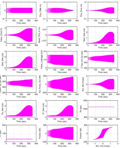
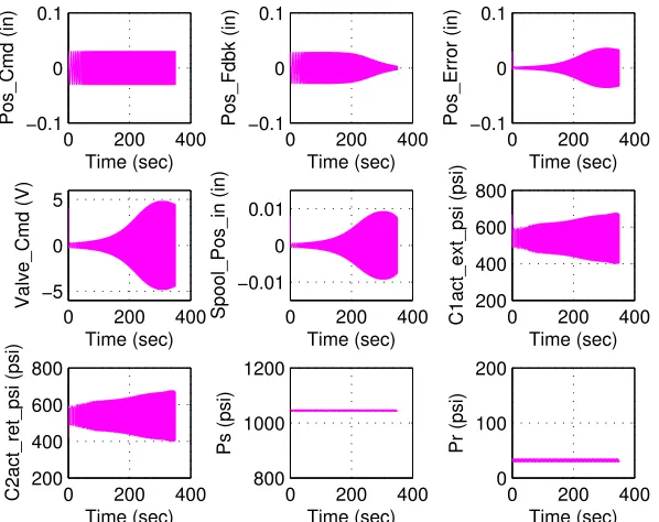
ex-components were modeled in three configurations - a Valve-Controlled Hy-draulic Actuator, an Electrohydrostatic Actuator, and lastly, a Hybrid DDV-EHA configuration. Both a nonlinear and linear model of each configuration is developed, verified, and validated against a similar experimental set up.

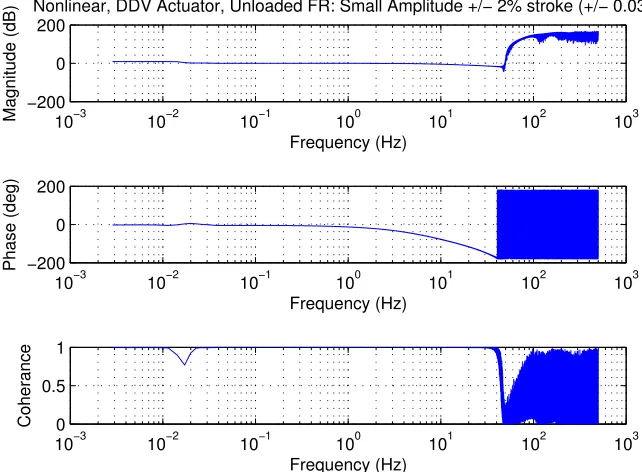
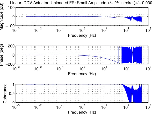
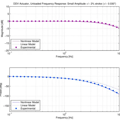
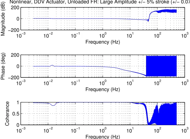
Each model was validated using four tests - low frequency and low am-plitude sinusoidal command, no load rate, small amam-plitude (2% stroke) un-loaded frequency response, and large amplitude (5% stroke) unun-loaded fre-quency response.

1.4 Assumptions of Theoretical Models

Assumptions were made for the theoretical models of the VCA, EHA, and DDV-EHA. For simplification purposes and proof of actuator archi-tecture concept only, proportional control was implemented on all three configurations within an actuator position loop with unity feedback gain. Loop gain was set based on the overall system performance aiming for ap-proximately 5% overshoot in step response position feedback and a similar closed loop crossover frequency around 6Hz for small amplitude unloaded frequency response.

The system model for the DDV assumes an ideal geometry spring-centered spool and simply uses a deadband width to account for the null region of the spool. The orifice flow equation assumes an initial coefficient of discharge for a sharp edge orifice approximately equal to 0.67.

Fluid is considered compressible, and therefore exhibits a capacitance in the hydraulic system. All fluid properties assume an ambient temperature of 68 degrees Fahrenheit. The change in temperature of the hydraulic fluid is assumed to be negligible over the simulation time interval.

In the case of the DDV-EHA model, the pressure controller was modeled using sump-pump theory, so the differential pressure thresholds are crucial system inputs.

(33)

The load actuator was modeled using a second order system model with inertial terms, generalized damping coefficients, and spring constants when applicable.

The linear models truly exhibit the ideal linear behavior of the system without introducing any leakage, friction, limit effects, and/or any other corrections for nonlinearities present in the systems.

1.5 Research Question

(34)

Chapter 2

Theoretical Direct Drive Valve Model

2.1 Development and Verification of Direct Drive Valve

Model

The DDV can be considered a four-way throttle valve with electric closed loop spool position control. Figure 2.1 shows a cut away of the Direct Drive Valve. The spool is spring centered and can be driven in both directions by a permanent magnet linear force motor, as shown in Figure 2.2. As the spool moves linearly within the bushing, supply and return pressure is metered in and out of the control ports associated with extend and retract flow to the equal area piston-cylinder [12].

Moog • D634-P Series 3

D

P

BENEFITS OF DIRECT DRIVE SERVO VALVES (DDV)

Directly driven by a permanent magnet linear force motor with high force level

No pilot oil flow required

Pressure independent dynamic performance Low hysteresis and low threshold

Low current consumption at and near hydraulic null Increased operation at limits (at high pressure drops)

Standardized spool position monitoring signal with low residual ripple

Electric null adjust

With loss of supply voltage, a broken cable, or an emergency stop, the spool returns to its spring centered position with-out passing a load move position.

D634-P Series Single Stage Proportional Valve

P T T2

A B

Y

Hydraulic symbol:

Symbol shown with electric supply on and zero command signal.

DIRECT DRIVEN PROPORTIONAL VALVE (DDV) OPERATING PRINCIPLE

The position control loop for the spool with position transdu-cer and linear force motor is closed by the integrated electro-nics. An electric signal corresponding to the desired spool posi-tion is applied to the integrated electronics and produces a pulse width modulated (PWM) current to drive the linear force motor. An oscillator excites the spool position transducer (LVDT), pro-ducing an electric signal proportional to spool position.

The demodulated spool position signal is compared with the command signal, and the resulting spool position error causes current in the force motor coil until the spool has moved to its commanded position, and the spool position error is reduced to zero. The resulting spool position is thus proportional to the command signal.

The linear force motor is a permanent magnet differential motor. The permanent magnets provide part of the required magnetic force. For the linear force motor, the current needed is considerably lower than would be required for a comparable proportional solenoid.The linear force motor has a neutral mid-position from which it generates force and stroke in both direc-tions. Force and stroke are proportional to current.

High spring stiffness and resulting centering force plus external forces (i.e. flow forces, friction forces due to contamination) must be overcome during out-stroking. During backstroking to center position, the spring force adds to the motor force and provides additional spool driving force which makes the valve much less contamination sensitive. The linear force motor needs very low current in the spring centered position.

Proportional solenoid systems require two solenoids with more cabling for the same function. Another solution uses a single solenoid, working against a spring. In case of current loss in the solenoid, the spring drives the spool to the end position by pas-sing through a fully open position. This can lead to uncontrol-led load movements.

PERMANENT MAGNET LINEAR FORCE MOTOR OPERATION

Null adjust cover plug

Valve connector

Spool

Integrated electronics

Position transducer Linear force motor Centering springs

Centering spring Permanent magnets Centering spring

Bearing Coil Armature Bearing

T A P B T2

(35)

15

Moog • D634-P Series 3

D

P

BENEFITS OF DIRECT DRIVE SERVO VALVES (DDV)

Directly driven by a permanent magnet linear force motor with high force level

No pilot oil flow required

Pressure independent dynamic performance Low hysteresis and low threshold

Low current consumption at and near hydraulic null Increased operation at limits (at high pressure drops)

Standardized spool position monitoring signal with low residual ripple

Electric null adjust

With loss of supply voltage, a broken cable, or an emergency

stop, the spool returns to its spring centered position

with-out passing a load move position.

D634-P Series Single Stage Proportional Valve

P T T2

A

B

Y

Hydraulic symbol:

Symbol shown with electric supply on and zero command signal.

DIRECT DRIVEN PROPORTIONAL VALVE (DDV) OPERATING PRINCIPLE

The position control loop for the spool with position transdu-cer and linear force motor is closed by the integrated electro-nics. An electric signal corresponding to the desired spool posi-tion is applied to the integrated electronics and produces a pulse width modulated (PWM) current to drive the linear force motor. An oscillator excites the spool position transducer (LVDT), pro-ducing an electric signal proportional to spool position.

The demodulated spool position signal is compared with the command signal, and the resulting spool position error causes current in the force motor coil until the spool has moved to its commanded position, and the spool position error is reduced to zero. The resulting spool position is thus proportional to the command signal.

The linear force motor is a permanent magnet differential motor. The permanent magnets provide part of the required magnetic force. For the linear force motor, the current needed is considerably lower than would be required for a comparable proportional solenoid.The linear force motor has a neutral mid-position from which it generates force and stroke in both direc-tions. Force and stroke are proportional to current.

High spring stiffness and resulting centering force plus external forces (i.e. flow forces, friction forces due to contamination) must be overcome during out-stroking. During backstroking to center position, the spring force adds to the motor force and provides additional spool driving force which makes the valve much less contamination sensitive. The linear force motor needs very low current in the spring centered position.

Proportional solenoid systems require two solenoids with more cabling for the same function. Another solution uses a single solenoid, working against a spring. In case of current loss in the solenoid, the spring drives the spool to the end position by pas-sing through a fully open position. This can lead to uncontrol-led load movements.

PERMANENT MAGNET LINEAR FORCE MOTOR OPERATION

Null adjust cover plug

Valve connector

Spool

Integrated electronics

Position transducer Linear force motor Centering springs

Centering spring Permanent magnets Centering spring

Bearing Coil Armature Bearing

T A P B T2

Figure 2.2: Linear Force Motor - Coil and Armature [13].

2.1.1 Spool Dynamics

(36)

an EHSV and therefore have a reduced chance of failure and exhibit lower internal leakage. Due to the absence of a hydraulic first stage, the spool position can be modeled assuming a spring-mass system of the spool with an additional inductive time constant for the linear force motor armature.

Kf s = Spool Stroke Valve Cmd



in

V (2.1)

xspool

Vcmd(s) =Kf s

✓ 1

⌧ps+ 1

◆ ✓

!n2

s2 _{+ 2}_⇣!

n +!n2

◆

(2.2)

⌧p...x + (2⇣!n⌧p+ 1) ¨x+ ⌧p!2n+ 2⇣!n x˙ +!n2x = Kf s!n2Vcmd (2.3)

Equation 2.2 represents the transfer function of the DDV spool with a spool stroke to electrical valve command proportionality constant in the nu-merator, second order spring-mass dynamics, and a lag attp, from the linear

force motor. The damping coefficient, z, natural frequency, wn, and time

constant, tp, were determined experimentally for various input amplitudes

[14, 15].

2.1.2 Orifice Flow Resistance

The control port flows within the spool were modeled using the sharp edge orifice flow equation represented by Equation 2.5 and 2.6. The orifice flow equation reveals a nonlinear relationship between volumetric flow rate and differential pressure. The sign function represented by Equation 2.4 accounts for the direction of flow since the DDV under consideration is a four-way valve [16].

Q = r

| P_|

(37)

K = ⇢hyd 2C2

dA2f low

(2.5)

GV = p1

K = Cd(xspool)(wslot)

s 2

⇢hyd

(2.6)

Valve gain, GV, is defined using the coefficient of discharge, area of flow,

and density of the hydraulic fluid. It is important to consider the ideal ge-ometry assumption being made. The flow holes are perfectly rectangular, and the diametrical clearance between the spool and bushing is negligible. Merritt suggests that four-way spool valves are often compared to a wheat-stone bridge circuit where the four arms are analogous to the four flow ports - supply pressure flow, return pressure flow, cylinder extend pressure flow, and cylinder retract pressure flow, as indicated by the hydraulic schematic and electrical circuit shown in Figure 2.3. The bridge is symmetric, and the resistance across all four arms is equivalent. In actual systems, however, the hydraulic path to the extend and return side of the actuator is often not equal considering sizing restrictions and manifold constraints. [15]

QC1ext =

8 < :

GVpPS C1ext

or , QC1ext 0

GVpC1ext PR

(2.7)

QC2ret =

8 < :

GVpPS C2ret

or , QC2ret 0

GV

p

C2ret PR

(2.8)

(38)

extend and retract pressure are compared against both supply and return pressure to determine proper flow direction.

(39)

2.2 Validation of Theoretical DDV Model

2.2.1 Experimental Laboratory Valve Testing Set Up

Figure 2.4: Valve Experimental Laboratory Test Set Up

The experimental laboratory set up shown above was used for frequency response and static testing. Pressure was supplied to the valve at 1000psi.

2.2.2 Optimization of Valve Transfer Function

An optimization routine using the built in Matlab function ’fminsearch’ was used to fit the third order valve transfer function represented by Equa-tion 2.2 to the experimental data using the cost funcEqua-tion shown below.

(40)

A weight of 100 is applied to the magnitude error due to the nature of its small magnitude relative to the phase error. Table B.1 represents the cost function value associated with amplitude dependent closed loop trans-fer function valve models. Higher fidelity was achieved with a higher order valve transfer function model. Refer to Table B.1 for closed loop valve transfer function optimization iteration values.

It is important to note that actuator level validation occurs within the 10Hz range due to a minimum coherence criteria of approximately 95%. Therefore the optimization routine was performed on experimental data within a lower frequency range (up to 50Hz for the DDV), as opposed to validation on the entire experimental frequency domain, which reaches a target frequency of 100Hz for the DDV case.

2.2.3 Unloaded Frequency Response

The dynamic response of the direct drive valve was tested with an input amplitude of ±0.5V to ±5.0V at a supply pressure of 1000psi swept from an initial frequency of 0.1Hz to a target frequency of 100Hz.

Figure 2.5 is the raw experimental frequency response of the DDV swept from 0.1Hz to 100Hz for input amplitudes from ±0.5V to ±5.0V. Figures 2.6 through 2.14 show the individual amplitudes of the experimental fre-quency sweeps shown in Figure 2.5. A plot of all experimental and theo-retical frequency response for input amplitudes from ±0.5V to ±5.0V swept from 0.1Hz to 50Hz is shown by Figure 2.15. Figure 2.16 plots the open loop frequency response of each theoretical optimized valve transfer func-tion from an input amplitude of ±0.5V to ±5.0V in a frequency domains from 0.1Hz to 100Hz. Figure 2.17 shows the final theoretical closed loop and open loop response of the small amplitude and large amplitude valve transfer function models, which are implemented in the theoretical actuator models.

(41)

100 101 102

−10

−8

−6

−4

−2

0 2

Experimental Frequency Response of Direct Drive Valve

Frequency (Hz)

Mag (dB)

100 101 102

−100

−80

−60

−40

−20

0

Frequency (Hz)

Phase (deg)

+/− 0.5V +/− 1.0V +/− 2.0V +/− 2.5V +/− 3.0V +/− 3.5V +/− 4.0V +/− 4.8V +/− 5.0V

Figure 2.5: Experimental Frequency Response of Direct Drive Valve from 0.1Hz to 100Hz

100 101

−1 0 1 2

Frequency Response of DDV +/− 0.5V Command

Frequency (Hz)

Mag (dB)

100 101

−60 −40 −20 0

2nd Order Approximation

(42)

100 101 −1

0 1 2

Frequency (Hz)

Mag (dB)

100 101

−60 −40 −20 0

2nd Order Approximation

Frequency (Hz)

Phase (deg)

Figure 2.7: Experimental and theoretical frequency response at 1.0V amplitude

100 101

−2 −1.5 −1 −0.5 0 0.5

Frequency (Hz)

Mag (dB)

100 101

−60 −40 −20 0

Frequency (Hz)

Phase (deg) _Experimental

Optimization

(43)

100 101 −2

−1.5 −1 −0.5 0 0.5

Frequency (Hz)

Mag (dB)

100 101

−60 −40 −20 0

Frequency (Hz)

Optimization

100 101

−6 −4 −2 0

Frequency (Hz)

Mag (dB)

100 101

−60 −40 −20 0

(44)

100 101 −6

−4 −2 0

Frequency (Hz)

Mag (dB)

100 101

−60 −40 −20 0

Frequency (Hz)

Optimization

100 101

−6 −4 −2 0

Frequency (Hz)

Mag (dB)

100 101

−60 −40 −20 0

Frequency (Hz)

Optimization

(45)

100 101 −6

−4 −2 0

Frequency (Hz)

Mag (dB)

100 101

−60 −40 −20 0

Frequency (Hz)

Optimization

100 101

−6 −4 −2 0

Frequency (Hz)

Mag (dB)

100 101

−60 −40 −20 0

(46)

100 101

−6

−5

−4

−3

−2

−1 0 1 2

Experimental and Theoretical Frequency Response of Direct Drive Valve

Frequency (Hz)

Mag (dB)

100 101

−70

−60

−50

−40

−30

−20

−10 0

Frequency (Hz)

Phase (deg)

(47)

100 101 102

−25

−20

−15

−10

−5

0 5 10 15

Theoretical Open Loop Frequency Response of DDV − Final TF Model

Frequency (Hz)

Mag (dB)

100 101 102

−200

−150

−100

−50

0

Frequency (Hz)

Phase (deg)

(48)

−150 −100 −50 0

Magnitude (dB)

100 101 102 103 104 105

−270 −225 −180 −135 −90 −45 0

Phase (deg)

Open Loop Frequency Response of Direct Drive Valve

Frequency (rad/sec)

Small Amplitude OL Small Amplitude CLTF Large Amplitude OL Large Amplitude CLTF

Figure 2.17: Frequency response of final valve transfer functions used in actuator model. Small amplitude model was used for small amplitude frequency response, and large ampli-tude model was used for large ampliampli-tude frequency response validation tests.

2.2.4 Flow Gain, Pressure Gain, and Leakage

(49)

experimental data reveals expected results with symmetric flow and pres-sure gain and maximum leakage within the null region of the valve.

(50)

Figure 2.20: Experimental and theoretical position plot.

(51)

Chapter 3

Theoretical Hydraulic Actuator Model

3.1 Development and Verification of DDV Actuator Model

Cylinder

Equal-Area

DDV-Controlled Hydraulic Actuator Schematic

Retract Pressure

Xducer

Extend Pressure

Xducer

DATA ANALYSIS

Manual Bypass Valve

Position Feedback

Supply Pressure

Xducer

Qext Qretr

Position Loop Closure

Bleed Port Bleed Port

Position Transducer

-+

Return Pressure

Xducer

Check Valve

DDV

Re

tr

ac

t

S

tr

ut

P

res

sur

e

Ex

te

nd

S

tr

ut

Pr

e

ss

u

re

Ac

tu

a

to

r

P

o

si

tio

n

Ret

ur

n

P

re

ss

ur

e

Supply Pressure

Position Command Position

Command

Pressure Supply

Leakage Path Phigh to Plow

Hydraulic Panel

Supply Pressure _Check

Valve

DDV Controller

Hydraulic Panel

Return Pressure

Pressure Return

(52)

The first configuration under investigation is a conventional valve-controlled hydraulic actuator - perhaps the simplest actuator design of all three config-urations. This actuator utilizes a direct drive valve, an actuating hydraulic piston-cylinder combination, and a hydraulic supply pressure source. Posi-tion feedback is achieved by a posiPosi-tion transducer, and the control error sig-nal is compensated for by the DDV which decides on the direction and rate of extend and/or retract flow to the actuator cylinder. The hydraulic power element in this configuration is the centralized hydraulic source, and the el-ement that provides flow is the direct drive valve. The hydraulic schematic for this configuration is shown in Figure 3.1.

3.1.1 Proportional Controller

A DDV includes closed loop position and pulse width modulated (PWM) drive integrated electronics to control spool position directly driven by a permanent magnet linear force motor. Pulse width modulation is a power control technique typically used for inertial electric devices in which rect-angular pulse waves at modulated widths are used to accomplish an average value waveform. The integrated electronics supply the linear force motor a PWM current based on an electrical signal input corresponding to desired spool position. The spools linear variable differential transformer (LVDT) provides an electric signal to the integrated electronics proportional to the current spool position. The desired spool position and actual spool position are then compared, and the error is reduced to zero as the spool travels to its correct position by electrical current supplied to the linear force motor coil [12].

xactcmd xactf dbk = Kp( xact) =eispool (3.1)

(53)

3.1.2 Friction Model

Friction is a highly complex and nonlinear phenomenon present in all hydraulic systems. It is important to characterize frictional effects due to its influence on the overall response of the actuator, represented by Equation 3.16. Friction is often accounted for in both a static and dynamic sense. Viscous and coulomb friction are common ways to model velocity depen-dent friction. However, they are often restrictive when considering the in-stantaneous change in applied frictional direction due to the severe depen-dence on the direction of travel. Therefore, a describing function with higher complexity should be used when modeling actuator friction considering the cyclic, ”turn-around,” behavior of the piston.

Fi = Mtx¨+Bx˙ +Ksx+ Ff +FLoad (3.2)

The LuGre friction model was implemented to appropriately model ac-tuator friction and can be described by Equations 3.3 through 3.5.

Ff = 0 + 1z˙ + 2vp (3.3)

˙

z = vp |vp|

g(vp)z (3.4)

g(vp) =

1

0

h

Fc + (Fs Fc)e (

vp

vs)

2i

(3.5)

The traditional stiffness, damping, and viscous coefficients are included by the s0, s1, and s2 terms. Another state, z, is introduced by the

(54)

non-linearity is accounted for in for two dynamic parameters, four static pa-rameters, a hydraulic stiffness coefficient, and a damping coefficient term. [17]

Although the LuGre friction model is highly complex, experimental data reveals an additional position dependent friction term. Figure 3.2 represents the application of the LuGre friction model alone and with an additional position dependent term. The frictional position dependence corrects for the discrepancy in cylinder pressure, but it does not significantly effect the overall response of the system.

0 5 10 15 20

−400

−200

0 200 400

Time (sec

Friction (lbf)

LuGre Friction Model

0 5 10 15 20

−400

−200

0 200 400

Time (sec

Friction (lbf)

LuGre + Position Dependent Friction Model

0 5 10 15 20

500 1000

Time (sec)

Cylinder Pressure (psi)

0 5 10 15 20

500 1000

Time (sec)

Cylinder Pressure (psi)

−1 −0.5 0 0.5 1

−400

−200

0 200 400

Actuator Velocity (in/sec)

Friction (lbf)

−1 −0.5 0 0.5 1

−400

−200

0 200 400

Actuator Velocity (in/sec)

Friction (lbf)

(55)

The position dependent term can be attributed to misalignment in the UUT rod and the load actuator rod, internal scoring within the cylinder, debris in the UUT cylinder and/or load actuator, etc. The uncertainty of the source and the insignificance of its presence in the overall system response suggests that the term be removed for further analysis.

3.1.3 Manifold-Cylinder Theoretical Model

The manifold-cylinder is the path between the DDV and the Unit Under Test (UUT) piston-cylinder.

Fluid Capacitance

The extend flow and retract flow ported by the metering edges of the DDV spool were determined using the orifice flow equation. The extend pressure and retract pressure within the UUT can now be determined using the continuity equation. Equation 3.6 represents the differential equation for the pressure inside a generic control volume. It is important to note that any large volume of compressible fluid within a hydraulic system is modeled as a capacitance. The time rate change of the control volumes fluid pressure is dependent upon the fluid capacitance[16]. The piston-cylinder is performing extend and retract cycles throughout this analysis, so the tim